Broadband matched-field processing: Coherent and incoherent
approaches
Cristiano Soaresa)and Se´rgio M. Jesusb)
SiPLAB–FCT, Universidade do Algarve, Campus de Gambelas, 8000-Faro, Portugal 共Received 2 January 2002; revised 7 October 2002; accepted 30 January 2003兲
Matched-field based methods always involve the comparison of the output of a physical model and the actual data. The method of comparison and the nature of the data varies according to the problem at hand, but the result becomes always largely conditioned by the accurateness of the physical model and the amount of data available. The usage of broadband methods has become a widely used approach to increase the amount of data and to stabilize the estimation process. Due to the difficulties to accurately predict the phase of the acoustic field the problem whether the information should be coherently or incoherently combined across frequency has been an open debate in the last years. This paper provides a data consistent model for the observed signal, formed by a deterministic channel structure multiplied by a perturbation random factor plus noise. The cross-frequency channel structure and the decorrelation of the perturbation random factor are shown to be the main causes of processor performance degradation. Different Bartlett processors, such as the incoherent processor 关Baggeroer et al., J. Acoust. Soc. Am. 80, 571–587 共1988兲兴, the coherent normalized processor关Z.-H. Michalopoulou, IEEE J. Ocean Eng. 21, 384–392 共1996兲兴 and the matched-phase processor关Orris et al., J. Acoust. Soc. Am. 107, 2563–2375 共2000兲兴, are reviewed and compared to the proposed cross-frequency incoherent processor. It is analytically shown that the proposed processor has the same performance as the matched-phase processor at the maximum of the ambiguity surface, without the need for estimating the phase terms and thus having an extremely low computational cost. © 2003 Acoustical Society of America. 关DOI: 10.1121/1.1564016兴 PACS numbers: 43.30.Wi, 43.30.Pc, 43.60.Cg关DLB兴
I. INTRODUCTION
The introduction of physical models in underwater acoustic signal processing has been one of the most signifi-cant advances ever in this field.1–3Defining a physical model for a given practical scenario allows for a consistent inclu-sion of a priori information on the signal estimation proces-sor. That a priori information consists of the environmental characteristics of the propagation scenario which, by means of the solution of the wave equation on that scenario, re-stricts the received acoustic pressure to a well-defined class of expected signals. It is that reduction of the class of ex-pected signals that provides the highest performance gain in terms of parameter estimation.
Since the definition of a physical model requires the knowledge共or the assumption兲 of a number of environmen-tally measurable quantities, the performance of the processor becomes dependent on those quantities. Conversely, if the emitted and received signals are known共or measurable兲 then it is, in principle, possible to estimate the environmental characteristics of the media of propagation—that is the base of the various matched-field 共MF兲 based techniques being developed in the last two decades: Matched-field processing
共MFP兲 for source localization, matched-field tomography 共MFT兲 for ocean properties and matched-field inversion 共MFI兲 for geoacoustic parameter estimation.
There are at least two aspects that emerge by their
re-levance to the success of MF based techniques: one is the ability of a given MF processor to accurately pinpoint the source location while rejecting sidelobes, and the other is the impact of erroneous or missing environmental information
共known as model mismatch兲 in the final parameter estimate.
This study addresses the first aspect, regarding sidelobe re-jection, while considering that the processor is working on a mismatch free situation. In that case, the capacity of detect-ing the correct acoustic field among very close similar can-didates 共the so-called discrimination兲 largely depends on the degree of complexity of the received acoustic pressure field. As an example, a single tone will have two discriminating parameters: the amplitude and the phase. If a broadband sig-nal is transmitted, there are as many amplitudes and phases as discrete frequencies, and the complexity of the received signal is naturally increased leading to a higher MF discrimi-nation. This problem is similar—but not equal—to the detec-tion problem encountered in classical spectrum estimadetec-tion.
There are a number of different ways to combine MF information across frequency that can be classified in two broad groups: the conventional incoherent methods, that are based on the direct averaging of the autofrequency inner products共average of real numbers兲 and the, say, less conven-tional methods, that perform a weighted average of the cross-frequency inner products where the weights are the fre-quency compensated phase shifts. The latter are generally called coherent broadband methods since they combine com-plex inner products.
Incoherent MF methods were first proposed by Bagge-roer et al.,4 where geometric averaging was found to be
ef-a兲Electronic mail: [email protected] b兲Electronic mail: [email protected]
fective to reduce ambiguous Bartlett and minimum variance
共MV兲 MFP sidelobes in a shallow-water simulation study.
The same principle was used in a countless number of stu-dies since then. More recently, the frequency domain coher-ent approach was first suggested by Tolstoy.5Michalopoulou recognized that incoherent processors discarded useful infor-mation contained in the off-diagonal terms of the cross-frequency data covariance matrix.6 Coherent Bartlett and MV processors based on the formulation of ‘‘supervectors’’ containing field vectors of the frequencies to be processed were proposed and successfully applied on tracking a sound source in the Hudson Canyon data set.7Czenszak and Krolik proposed a coherent minimum variance beamformer with en-vironmental perturbation constrains共MV–EPC兲 designed for a short vertical array.8Very recently Orris et al. proposed a matched-phase coherent processor that accounts for the rela-tive phase relationships between frequencies.9Those phases are assumed to be unknown and are searched as free param-eters.
In that classification, time domain methods play a differ-ent role but can, to some extdiffer-ent, be included in the coherdiffer-ent class. Time domain methods were first suggested by Clay10 under the form of an optimum matched-filter for source lo-calization. The same technique was used by Li et al.11 in laboratory experimental data. Also Frazer et al.12 tested Clay’s technique with simulated data and a single hydro-phone. In 1992, Miller et al.13showed, with computer simu-lations, that it is possible to localize short duration acoustic signals in a range-dependent shallow water environment. The same approach was followed by Knobles et al.14with bottom moored sensors using a broadband coherent matched-field processor proposed by Westwood.15Time domain source lo-calization was actually achieved with real data by Brienzo
et al.16using data received on a vertical array in a deep water area on the Monterrey fan. The technique used was a com-bination of time domain filtering for each sensor 共matched-filter兲 and then a space domain beamformer.
Despite the considerable amount of work on broadband methods there is a lack of understanding on why and when a coherent method provides a better detection or localization performance than an incoherent method. This is the main topic addressed in the present study, that starts by presenting a physical-based linear data model with suitable random per-turbation terms as opposed to the traditional fully stochastic model. Under this model, it is shown that the advantage of using the cross-frequency terms resides in its ability to reject noise, while its disadvantage is that the result is limited by the correlation of the random phase terms together with the deterministic correlation of the channel response across fre-quency. An efficient algorithm for combining cross-frequency information is derived that is shown to have an equivalent localization performance than that of the matched-phase coherent processor with a much lower com-putational burden. Then, the performance of the coherent and incoherent processors are compared for different number of frequencies using simulated data. Real data analysis is pre-sented to support the physical-based model as well as for justifying the distributions of the random perturbation terms. Finally, a real data example shows the effect of a wise
selec-tion of frequency bands on the final match of the model to the data.
II. DATA MODEL
A. The physical data model
A widely used data model for M farfield point sources emitting narrowband signals received in a L-sensor array is given by
y共t兲⫽A共兲s共t兲⫹u共t兲, 共1兲
where y(t) is the L-sensor array received acoustic pressure,
A() is the L⫻M steering matrix, which entries are the appropriate delays for each array sensor and each source m at bearing m, s(t) is an M-dimensional vector with the M
source inputs at time t and u(t) is the observation additive noise. A common assumption is to consider that the additive noise is white, Gaussian, zero-mean and uncorrelated with the signals s(t), that themselves are zero-mean and uncorre-lated stochastic processes. This model is useful for describ-ing a field of dependent noise sources emittdescrib-ing through a nondispersive unbounded media and received on a horizontal array. When dealing with shallow water dispersive scenarios, deterministic sources and nonhorizontal arrays this model is unable to account for the complexity of the received field as a mixture of correlated共partially兲 deterministic signal reflec-tions from sea bottom and sea surface.
An alternative approach is to start from the wave equa-tion and directly calculate its soluequa-tion with appropriate boundary conditions and environmental assumptions 共e.g., azimuth and range independent isotropic media, spatial point source, etc.兲. In a cylindrical two-dimensional coordinate system, the acoustic pressure measured at receiver depth zl
due to a point source at range r and depth zs can be written17
p共zl,t;r,zs兲⫽ ⫺i 2
冕
兺
j⫽1 JM s共兲⌿j共zl兲⌿j共zs兲冑
rkj ⫻e⫺i共kjr⫺/4兲⫺␥jreitd, 共2兲where s() is the source spectrum, 兵⌿j( ), j⫽1,...,JM其 are
the waveguide mode functions, and kj and␥j are the mode
horizontal wave numbers and mode attenuation coefficients, respectively; JM is the number of discrete modes supported
by the waveguide.
Under the ray approximation the received acoustic pres-sure, using the same notation, can be written as
p共zl,t;r,zs兲⫽
1 2
冕
兺
j⫽1JR
ajs共兲e⫺ijei共t⫹兩/2兩兲d, 共3兲
where the number of eigenrays JR, the ray amplitudes ajand
the delaysj, fully characterize the propagation channel for
the specific source and receiver locations, (0,zs) and (r,zl),
respectively.
Assuming the propagation channel as a linear filter, al-lows for writing the received signal as the frequency product between the source signal s() and the channel transfer function h(), defined as the sum of modal terms共or rays兲
for a particular source–receiver location. Thus, a suitable model for the array-received signal from an harmonic source at frequencywould be
y共zl,;r,zs兲⫽h共zl,;r,zs兲s共兲⫹u共zl,兲, 共4兲
where u(zl,) is a zero-mean stochastic process
represent-ing additive observation noise and where h(zl,;r,zs) can
be easily deduced either from 共2兲 or from 共3兲 depending on which model—normal mode or ray model—is being used. It is a common assumption to consider the observation noise to be wide-sense time stationary. Taking into account the Fou-rier transform properties for sufficiently long observation times it can be considered that the frequency samples of u are asymptotically uncorrelated.
If the source input s(t) is deterministic, signal detection using model 共4兲 becomes a problem of detecting a determi-nistic signal in white noise, which optimal solutions are well known.
In the past decade, with the development of methods for acoustic inversion using deterministic signals, it has been observed that repeated emissions at very high SNR resulted in successive receptions suffering rapid changes in short time intervals possibly caused by small scale environmental per-turbations, source and/or receiver motion, and sea surface and bottom roughness, which, partially or all together, con-tribute to unmodeled fluctuations in the signal part of 共4兲.
Since such changes cannot be attributed to the noise due to the high SNR, a complex random factor ␣⫽兩␣兩exp(j) can be included such that the data model is written as
y共,0兲⫽␣共兲h共,0兲s共兲⫹u共兲, 共5兲 where a more compact notation has been adopted by intro-ducing a vectorial notation for the L-sensor array as y
⫽关y(z1),y (z2),...,y (zL)兴t and similar definitions for h and u, the channel transfer function and the additive observation
noise, respectively; s() is the source spectrum at frequency
and0 is a vector with the relevant parameters under es-timation. The noise process u is assumed to be uncorrelated from sensor to sensor and with random factor ␣. Note that random factor␣is space invariant but is assumed to be fre-quency dependent. For the design of optimal estimators it is useful to consider that ␣is zero-mean and Gaussian distrib-uted. Whether that assumption is verified in practice is the subject of the next section.
B. Random signal perturbation factor
This section deals with the distribution of the random signal perturbation factor␣, introduced in the linear physical model 共5兲. It is a common assumption to consider that ran-dom factor to be complex zero-mean Gaussian distributed,4 which implies that the module of␣ follows a Rayleigh dis-tribution and that its phase is uniformly distributed in关⫺,
兴.18 In case that the real and/or imaginary parts of the
acoustic pressure are not zero mean then the envelope fol-lows a Rice distribution while the phase term does not ap-pear to be uniform nor Gaussian distributed 共see Appendix A兲.
In order to obtain an empirical distribution of the signal random perturbation, only possible using real data, one has
to, first, assume that the signal-to-noise ratio共SNR兲 is suffi-ciently high, to be able to neglect the influence of the noise
u, and second, assume that the deterministic part of the
sig-nal, i.e., h(,0)s() is time-stationary or slowly varying.
Under these two assumptions a possible estimator,␣ˆ , of the
random factor␣at frequencyis
␣ˆn⫽
yn y0⬇
兩␣n兩
兩␣0兩ej共n⫺0兲, 共6兲
where yn, ␣n, andn are obtained for time snapshot n and for an arbitrary frequency and receiver. This would imply that the distribution of 兩␣ˆ兩 would be Rayleigh or Rice
de-pending on whether␣ is zero-mean or not with, however, a change on the amplitude axis due to the normalization con-stant 兩␣0兩. As an alternative and, if the stationarity assump-tion for h(,0)s() is suspected not to hold, another
esti-mator can be sought using a time sliding estiesti-mator as
␣ˆn⫽ yn yn⫺1⬇ 兩␣n兩 兩␣n⫺1兩 ej共n⫺n⫺1兲. 共7兲
In this case the interpretation is a bit more elaborated since the module of ␣ is the ratio of two Rayleigh共or Rice兲 ran-dom variables and the phase term is the difference between two uniform variables if␣ is zero mean. It is shown in Ap-pendix B that the ratio of two independent Rayleigh distri-buted random variables gives a nearly Cauchy distridistri-buted random variable and that the difference of two uniformly distributed and independent random variables gives a prob-ability density function 共pdf兲 for the resulting random vari-able that is triangular in关⫺2, 2兴. Results obtained on real data using estimators共6兲 and 共7兲 are shown in Sec. VI.
III. SECOND ORDER STATISTICS AND BROADBAND MODEL FORMULATION
The correlation matrix can be directly written from 共5兲 as Cy y共,0兲⫽E关y共,0兲yH共,0兲兴 ⫽E关兩␣共兲兩2兴兩s共兲兩2h共, 0兲hH共,0兲 ⫹u 2 共兲I, 共8兲
where all terms have been previously defined and superscript
H denotes conjugate transpose. Equation共5兲 gives the
essen-tial description of the received data model in the narrowband case. When a time-limited signal共impulse兲 is emitted by the source, a significant band of frequencies of the acoustic channel is excited giving rise to the need for a broadband formulation. In order to introduce, as much as possible, a common frame for the narrowband and broadband cases, we define an extended vector as
yᠪ⫽关yT共1兲,yT共2兲,...,yT共K兲兴T, 共9兲
where superscript T denotes matrix transpose and K is the total number of discrete frequency bins. In that case, the broadband model can be written as
where s˜ᠪ is a K-dimensional random vector which entries are s(k)␣(k), i.e., the source spectrum multiplied by the
ran-dom perturbation factor at each frequencyk苸关1,K兴; the
matrix H(0) is H共0兲⫽
冋
h共1,0兲 0 ¯ 0 0 h共2,0兲 ¯ 0 ] ] ] 0 0 ¯ h共K,0兲册
, 共11兲where the noise extended vector uᠪ has an obvious notation similar to共9兲. It is interesting to write the correlation matrix for model共10兲, which cross-frequency block matrix is given by Cy y共i,j兲 ⫽
冦
兩s共i兲兩2h共i,0兲h共i,0兲HE关兩␣共i兲兩2兴⫹u 2共 i兲I, i⫽ j, s共i兲s*共j兲h共i,0兲hH共j,0兲E关␣共i兲␣*共j兲兴, i⫽ j, 共12兲where the term E关␣(i)␣*(j)兴 denotes the correlation of
the perturbation factor across frequency. Note that unlike the autofrequency entries (i⫽ j) the cross-frequency terms (i
⫽ j) are noise free. This is due to the well-known property of
the Fourier transform for time-stationary processes that gives uncorrelated cross-frequency bins which might be also useful if spatially correlated noise is present. In practice, with finite observation time, that property is only asymptotically veri-fied, which is often sufficient. In expression 共12兲, for i⫽ j, there are three contributions: the source cross-spectrum term
s(i)s*(j), the cross-frequency acoustic channel structure
term h(i,0)hH(j,0) and the perturbation factor
corre-lation E关␣(i)␣*(j)兴. The first term is source dependent and will not be of concern here. The second term is channel dependent and may significantly vary with environmental conditions, source position 共range and depth兲 and receiving array geometry. The third term on expression 共12兲, for i
⫽ j, concerns the correlation of the perturbation factor and is
impossible to obtain from simulations.
IV. BARTLETT MATCHED-FIELD PROCESSING
The Bartlett processor is possibly the most widely used estimator in MF parameter identification. The parameter es-timate ˆ0 is given as the argument of the maximum of the
functional
P共兲⫽E关wˆH共兲y共0兲yH共0兲wˆ共兲兴, 共13兲
where the replica vector estimator is determined as the vector
w() that maximizes the mean quadratic power,
wˆ共兲⫽arg max
w E关w
H共兲y共0兲yH共0兲w共兲兴, 共14兲
subject to wH()w()⫽1. In the narrowband case, using model 共5兲 in 共14兲 gives the well-known nontrivial solution
wˆNB共兲⫽
h共兲
冑
hH共兲h共兲, 共15兲where the denominator is a normalization scalar and the nu-merator contains the signal structure as ‘‘seen’’ at the receiv-ing array. This is simply the classical matched filter for the particular parameter location . Substituting 共15兲 in 共13兲 gives the well-known generalized conventional narrow band beamformer for parameter. If the search is made overand the maximum is selected, then an optimum mean least-squares estimateˆ0 of0 is obtained.
In the broadband case, the estimator of the replica vector is given in terms of frequency extended vectors using model
共10兲, thus
wˆᠪBB共兲⫽arg maxwᠪ 兵wᠪH共兲H共0兲E关sᠪ˜sᠪ˜H兴HH共0兲wᠪ共兲其,
共16兲
where the expectation of the signal matrix s˜ᠪs˜ᠪH relates to the correlation of the perturbation factor ␣ across frequency, weighted by the source power cross spectrum s*(i)s(j).
No closed form for wˆᠪBB() can be given in this case without
explicit knowledge of that signal matrix. There are a number of possible implementations that represent suboptimal ver-sions of共16兲 with different assumptions for the structure of the perturbation correlation and signal weighting matrix. A few cases are reviewed in the next section and a new com-putational effective alternative to existing techniques is also proposed.
A. Broadband incoherent processor
The so-called incoherent broadband Bartlett processor, originally proposed in Ref. 4, implicitly assumes that the random factor is simply E关␣(i)␣*(j)兴⫽␣
2␦
i j, i.e., that
the random perturbations are uncorrelated across frequency and have a constant power. Using that expression of the cor-relation of␣in共12兲, plugged in 共16兲 and solved for w gives
wˆᠪinc共兲⫽ H共兲sᠪ
储H共兲sᠪ储, 共17兲
where sᠪ is a K-dimensional vector which entries are s(k).
Thus, by replacement into共13兲, allows to obtain the proces-sor expression Pinc共兲⫽␣ 2兺 k⫽1 K 兩s共 k兲兩2hH共k,兲Cy y共k,k兲h共k,兲 储H共兲sᠪ储2 共18兲
which is nothing more than a source power weighted sum of the diagonal matched-filtered autofrequency block matrices of the extended correlation matrix Cy y. Notice that if␣had been assumed to be frequency dependent, a factor ␣(k) would appear as weighting the terms in the summation in
共18兲. In the case of a flat source power spectrum, Eq. 共18兲
reduces to a simple summation of the quadratic terms across the discrete band of frequencies. When the source power spectrum is unknown but not flat, an unweighted incoherent processor is generally used which leads to the suboptimal incoherent broadband conventional estimator proposed in Ref. 4.
B. Broadband coherent processor
Although there is good evidence that for many of the real underwater propagation channels most of the energy is concentrated along the main diagonal of the cross-spectrum correlation matrix 共the autofrequency terms兲 it is also clear that the same autofrequency terms would carry the noise power as it can be seen in expression共12兲. One of the moti-vations when performing coherent processing is to take ad-vantage of the noiseless cross-frequency terms of共12兲. These cross-frequency terms have no noise but the signal informa-tion they contain may also be reduced, according to both the channel cross-frequency structure and the cross-frequency correlation of the random perturbation factor, as explained in the preceding section. This explains why in most studies, concerned with coherent processing, only the cross-frequency off-diagonal terms were used, excluding the diag-onal autofrequency information.9There are actually several broadband coherent processors depending on the assump-tions made for approximating the cross-frequency perturba-tion terms of the signal matrix E关s˜ᠪs˜ᠪH兴 of 共16兲.
1. Coherent normalized processor
The coherent normalized processor共COH–N兲 has been proposed by Michalopoulou7,19and attempts to eliminate the source spectrum–perturbation weighting across frequency. At each frequencyi, a normalized model vector is defined
as
nx共i,0兲⫽
x共i,0兲
xl共i,0兲
, 共19兲
where xl(i,0) is the signal received at sensor l. The
choice of l depends on the actual signal-to-noise ratio共SNR兲 at that particular sensor. In a high SNR situation, if the noise contribution at sensor l is neglected, the normalized data model becomes
nx共i,兲⬇nh共i,0兲⫹ u共i兲
hl共i,0兲s共i兲␣共i兲
. 共20兲 Matching this model with an extended normalized replica vector yields a perfect match for the signal and a strongly correlated structure for the noise field due to the noise term in共20兲. In that case the coherent-normalized replica vector is written as
wˆcoh-n共i,兲⫽nh共i,兲⫽
h共i,兲
hl共i,兲
, 共21兲
and using that expression in the Bartlett processor gives
Pcoh-n共兲 ⫽
兺
i⫽1 K兺
j⫽1 K nhH共i,兲nh共i,0兲nh H 共j,0兲nh共j,兲 ⫹nh H共 i,兲Cnunu共i,j兲nh共j,兲, 共22兲 where Cnunu(i,j) is the cross-frequency correlation
ma-trix of the normalized additive noise vector nu defined in the
second term of 共20兲. Expression 共22兲 shows a perfectly co-herent match for the signal model part when ⫽0, and a
noise term residual which is a constant when i⫽ j, due to the
white noise assumption, and has a correlation structure for
i⫽ j that is highly dependent on the cross-frequency
correla-tion of the perturbacorrela-tion ␣共兲.
2. Matched-phase coherent processor
Another approximation to the broadband coherent pro-cessor has been recently proposed by Orris9 where the cor-relation terms are explicitly included in the replica vector as unknowns and have therefore to be estimated. A new replica vector is defined as
wᠪcoh-mp共兲⫽关hT共1,兲ejˆh共1兲,...,hT共K,兲ejˆh共K兲兴T,
共23兲
where the phase terms关ˆh(k);k⫽1,...,K兴 are the estimates that maximize the output power upon summation over sensor and frequency. Taking into account that, when carrying out that summation, each term has its complex conjugate, the energy contained in the imaginary part is lost. The unknown phase terms h are estimated in such a way as to minimize
that loss which, ideally, requires the unknown phase terms to be symmetric to the phase of the signal matrix terms in共12兲. If that is achieved all terms turn into real numbers and the sum is carried out in phase. In that case, and for a flat spec-trum source, this processor is optimum. Replacing共23兲 in the Bartlett processor expression gives
Pcoh-mp共兲⫽
兺
i⫽1 K兺
l⫽1 K hH共i,兲Cy y共i,l兲 ⫻h共l,兲e⫺ j关ˆh共i兲⫺ˆh共l兲兴. 共24兲In practice, the problem associated to the matched-phase pro-cessor, according to Orris,9is the computation load necessary to obtain the estimates ˆh of the phase shifts h, for an
exhaustive search over a realistic parameter space. That com-putation load is of the order of o⫽JK⫻M⫻N, where J is the
number of samples for the phase in关0, 2兴, K is the number of frequencies and M⫻N is theparameter search grid共e.g., range versus depth兲. In practice, and as mentioned by Orris,9 if the source location and relative phases have to be exhaus-tively searched, computation complexity limits the number of frequencies to K⫽3 while for a larger number of frequen-cies efficient search algorithms 共e.g., simulated annealing兲 were proposed.
C. The cross-frequency incoherent processor
The cross-frequency incoherent processor is proposed in this paper and represents an alternative to overcome the com-putational burden of the matched-phase processor while keeping the same performance. This processor stems from the simple idea that the phase corrections for the surface maximum (⫽0) are
h共i兲⫺h共j兲⫽⬔s共i兲s*共j兲E关␣共i兲␣*共j兲兴, 共25兲
for all i, j⫽1,...,K which can be seen by direct inspection of
共12兲 and where ⬔ means ‘‘phase of.’’ When these corrections
are correctly set the value of the maximum is just the sum of a series of real numbers, which are the modules of the qua-dratic terms across frequency, i.e.,
Pinc-xf共兲⫽
兺
i⫽1 K兺
j⫽1 K 兩hH共 i,兲Cy y共i,j兲h共j,兲兩. 共26兲The value of the maximum of the ambiguity surface obtained with共26兲 is exactly the same as that obtained with 共24兲 with absolutely no phase parameter search. Therefore, the peak would have the same height and the same location, however the aspect of the resulting surface would be much different between the cross-frequency and the matched-phase proces-sors: the former would have a smooth appearance, much like the incoherent processor, and the latter would have extremely narrow peaks distributed along the surface with, however, an overall envelop that is very similar to that of the cross-frequency incoherent processor. Examples on simulated data are given in the next section.
V. SIMULATION RESULTS
This section shows a few simulated data examples of the application of broadband MF processors to source localiza-tion. The data was simulated using the C-SNAP model20in a 80 m deep range-independent shallow water scenario similar to that of the ADVENT’99 experiment.21The acoustic source is placed at 76 m depth and at 5 km range from a 32-sensors vertical array. The source is emitting a series of multitones between 300 and 600 Hz with 100 Hz increment. The signals were generated in the frequency domain using 共4兲 with an SNR of ⫺8 dB and the correlation matrix was estimated using 32 snapshots. The noise level was set accordingly to the following SNR definition:
SNRdB⫽10 log兺k⫽1 K s 2 共k兲 兺k⫽1 K u 2共 k兲 , 共27兲 where s 2 共k兲⫽ E关储h共zl,k,r,zs兲s共k兲储2兴 L 共28兲 and u 2共 k兲⫽ E关储u共k兲储2兴 L . 共29兲
Figure 1 shows the range-depth ambiguity surfaces ob-tained for the above referred broadband Bartlett processors,
Pinc共a兲, Pcoh-n 共b兲, Pcoh-mp 共c兲, and Pinc-xf 共d兲. In cases 共b兲, 共c兲, and 共d兲 only the cross-frequency terms were used. As
expected, the incoherent processors共a兲 and 共d兲, gave similar smooth surfaces with a lower sidelobe structure for the cross-frequency processor. The coherent processors共b兲 and 共c兲 also gave similar responses with a large number of very narrow peaks共up to only 1 m wide in range兲 that are due to a perfect alignment of the surfaces for all grid points. By formulating the matched-phase and the incoherent cross-frequency pro-cessors in terms of normal modes, it can be shown that the corresponding ambiguity surfaces are oscillating functions of the distance modulated by an amplitude factor that is the same in both processors. The peaky structure shown by the coherent processors results from a periodic phase alignment of the correlation terms at each pair of frequencies. At low SNR the coherent normalized processor共b兲, rapidly degrades due to the SNR limitation pointed out in 共20兲. As explained above the matched-phase and the cross-frequency incoherent processors have analytically the same source detection per-formance with comparable peak-to-sidelobe ratios of 2.5 dB and 2.0 dB, respectively. Note that for the coherent proces-sors a subsampling of the ambiguity surface in range can hide the sidelobe structure. The detection performance of the FIG. 1. Ambiguity surfaces computed with synthetic data generated without perturbation factor for the ADVENT’99 scenario at frequencies 300, 400, 500, and 600 Hz, at SNR⫽⫺8 dB and for the following processors: 共a兲 incoherent conventional, 共b兲 coherent normalized, 共c兲 matched-phase coherent, and 共d兲 incoherent cross frequency.
cross-frequency incoherent processor is shown in Fig. 2 for the model without perturbation. This performance was mea-sured in terms of probability of correct source localization by determining how often the peak appeared at the correct lo-cation in 50 realizations. The environment is always that of the ADVENT’99 experiment. The effect of increasing the number of frequencies within a relatively small frequency band of 100 Hz around 550 Hz is shown in plots共a兲 to 共c兲 of Fig. 2, where the number of frequencies is 4, 7, and 16, respectively. It can be noticed that the performance of the cross-frequency incoherent processor is always superior to that of the conventional 共autofrequency兲 incoherent proces-sor due to the higher number of frequencies involved and to the noise immunity, despite the inevitable decrease in chan-nel structure power transmission at certain cross frequencies off the main diagonal. The number of ambiguity surfaces increases as K for the incoherent processor and as K⫻(K
⫺1)/2 for the cross-frequency incoherent processor. That
fact results in a steady increase of the difference in perfor-mance with the number of discrete frequencies from 4 to 7 and then to 16. With 16 frequencies there is a gain in detec-tion performance estimated to approximately 4 dB at useful detection probabilities. The result shown in plot共d兲 was ob-tained for a number of frequencies equal to 16关the same as in plot共c兲兴 but within a frequency band enlarged to 300 Hz, always centered at 550 Hz. The result is that there is a slight decrease of the performance of both processors, while that decrease is stronger for the incoherent cross frequency, thus there is a net loss of performance of the cross-frequency processor relative to the incoherent autofrequency processor. Other tests performed for relatively small number of closely spaced discrete frequencies clustered around center frequen-cies along the whole band gives better results than uniformly distributed frequencies in the same band.
In practice, with real data, these performance predictions obtained in simulation have to be balanced by the correlation
of the perturbation factor across-frequency contributing to a net decrease of performance when enlarging the bandwidth around a given center frequency. That fact clearly favors the solution of using the proposed cross-frequency incoherent operating in closely spaced frequencies clustered at various frequencies in the useful band.
VI. A REAL DATA EXAMPLE
The ADVENT’99 data set was used as to provide a real world example for the assertions made in the preceding sec-tions. The ADVENT’99 experiment took place during the month of May of 1999, in a nearly range independent area on the Strait of Sicily, Italy. The approximate depth of the area was 80 m and the acoustic signals were transmitted from a bottom mounted sound source and received on a 31-hydrophone vertical array. Various signal sequences at differ-ent frequencies and repetition rates were used. Also, the ver-tical array was successively located at ranges of approximately 2, 5, and 10 km. A complete description of the experimental setup can be found in Siderius et al.21
A. The perturbation factor
In order to justify the perturbation factor distribution, a signal tone at 200 Hz was extracted from the time series recorded during 18 hours on a mid-water-depth hydrophone at 10 km range from the signal source. The signal-to-noise ratio is expected to be⬎20 dB at that frequency, and the additive noise is assumed negligible compared to the signal term. Figure 3 shows the estimated pdf’s based on the histo-grams obtained for the module—共a兲 and 共c兲—and for the phase—共b兲 and 共d兲. In plots 共a兲 and 共b兲, module and phase pdf’s are estimated using the normalization proposed in共6兲. It can be seen that the module is approximately Rayleigh distributed, with parameter⫽1 due to the normalization by
y0, while the phase is noncentered共also due to the
normal-FIG. 2. Probability of correct source localization obtained on ADVENT’99 conditions simulated data for the broadband incoherent processor共dashed兲 and broadband cross-frequency processor共continuous兲 in the frequency band 关500, 600兴 Hz for the following number of frequencies: 4共a兲, 7共b兲, 16共c兲 and also 16 but in the band关400, 700兴 Hz.
ization兲, almost uniform in 关⫺,兴 with an outstanding peak at⫽⫺0.5 rad of unknown nature. Instead, the sliding nor-malization of共7兲, applied in the same data set, provides the results shown in plots共c兲 and 共d兲 for the module and phase, respectively. The module—plot 共c兲—is in this case approxi-mately distributed according to the approximate Cauchy given by 共B2兲, while that of the phase—plot 共d兲—does not resembles to a triangular function as a result from the differ-ence of two uniformly distributed random variables. The dis-tribution is approximately symmetric in关⫺2, 2兴, but has a much narrower peak than expected for a triangular shaped pdf. Due to the complicated form of the expression of the phase pdf in the noncentered case关Appendix A, Eq. 共A14兲兴, it is difficult to theoretically predict what could be the ex-pected pdf for the phase random variablen⫺n⫺1. Some
numerical simulations using expression 共A14兲 and realistic values forsuggest that a bell-shaped centered pdf as that of Fig. 3共d兲 can most likely be obtained for ma⬎0 and mb
⬇0. 关Note that the empirical distribution of Fig. 3共d兲 is,
ac-cording to the theory, the autocorrelation of two identical pdf’s as that obtained in共A14兲兴. A similar behavior was veri-fied on the ADVENT’99 data set at various frequencies in the interval 关200,1500兴 Hz, with however, an increasing broadening of the peak of the phase pdf with frequency. A broader pdf means a larger value for which is a well known effect leading to highly variable phase shifts at high frequency making it difficult to accurately predict. This dis-cussion brings a key question for broadband applications, that is to determine which is the degree of correlation of the signal across frequency.
Using the same ADVENT’99 data set along a wide fre-quency band 关200,1600兴 Hz, the correlation of the perturba-tion factor using the normalizaperturba-tion 共6兲 was estimated. The result is shown in Fig. 4 where a broad diagonal along the whole frequency band can be observed. Additional effects of frequency bandpass of the two transducers used to cover this wideband of frequencies can be seen on the artificially low
levels of energy in the diagonal at about 800 Hz, which is the overlap transit in frequency band.
In order to obtain a complete view of the received signal correlation along frequency one has to add the deterministic effect of the channel correlation. As an example, a scenario similar to that of the ADVENT’99 was simulated to compute the cross-array coherence of the acoustic channel across the frequency band of interest. Figure 5 shows the result of the expression
Ch共i,j兲⫽hH共i兲h共j兲, 共30兲
for i,j苸关200,1600兴 Hz. It can be easily noticed from
that figure that the energy is not concentrated on a single diagonal but on a band of frequencies around that diagonal. The bandwidth varies with frequency and with source– receiver geometry 共not shown兲, e.g., it tends to be larger at longer ranges due to stronger multipath. There is also a
sig-FIG. 3. Estimated probability density functions of signal perturbation factor from the ADVENT’99 data set at 200 Hz: using first element normalization for the module共a兲 and phase 共b兲; using a sliding window along time for module 共c兲 and phase 共d兲.
FIG. 4. Estimated correlation of normalized signal perturbation factor over the band 200–1600 Hz using the LFM data of the ADVENT’99 experiment at 5 km source–receiver range.
nificant amount of energy well apart from the diagonal due to mode interference.
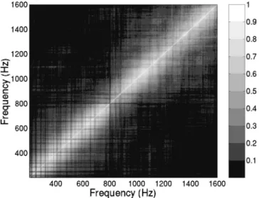
These two last Figs. 4 and 5 can be compared by means of a third figure that is the frequency correlation matrix of the signals received at 5 km range during the ADVENT’99 sea trial 共Fig. 6兲. The first comment is that the resemblance between this figure and that obtained with simulated data is striking. It appears that the cross-frequency energy spread out of the diagonal is largely attenuated when compared with the synthetic data example, that is particularly true in the low frequency range but is also evident at high frequencies where the main diagonal lobe is narrower. An estimation of the effective ⫺3 dB bandwidth shows that at least 100 Hz are available throughout the analyzed frequency range between 200 and 1600 Hz. Comparison of Figs. 5 and 6 should be done under the assumption that the latter contains informa-tion on the source spectrum level that might alter the result. Note that the values plotted in the last three figures were normalized, so there is no information on the relative levels of each term on the final observed signal.
B. Broadband MFP
The results shown in the preceding section suggest that due to the limited correlation of the perturbation factor, cross-frequency broadband processors should preferably op-erate on relative narrow bands of 100 or 200 Hz than on wide frequency bands. In order to illustrate that point with a real data example, a series of vertical array observations at 5 km range and in the band 400–1000 Hz was drawn from the ADVENT’99 data set and processed with the proposed cross-frequency incoherent Bartlett processor for range-depth source localization purpose. Figure 7 shows the Bar-tlett power results obtained during approximately five con-secutive hours of data for two processing schemes: the seven tones at 100 Hz spacing between 400 and 1000 Hz were processed in a single frame 共*兲 and the same tones were processed in three groups of three frequencies each 共䊊兲— groups 共400,500,600兲, 共600,700,800兲, and 共800,900,1000兲. The number of cross-frequency terms is 21 in the first scheme and nine in the second scheme. Despite that differ-ence the Bartlett power, i.e., the value of the normalized peak in the final ambiguity surface at the correct source location, is always higher for the processing in the clustered band than in the wide band. The range-depth source localization perfor-mance was the same for both processors. The grouping of frequencies in a limited band acts as an automatic scheme to exclude the correlation terms that yield worst SNR at the processor’s output caused by low cross correlation of the signal components.
VII. CONCLUSION
For many years, underwater acoustic signal processing was devoted to the detection and/or localization of narrow-band or broadnarrow-band random sources using a multisensor hori-zontal array. Localization here meant bearing estimation, which was the main scope of a wide, yet powerful, suite of techniques. That situation has dramatically changed with the wide spread of physical model codes being able to predict the acoustic channel propagation characteristics at various FIG. 5. Channel coherence of simulated acoustic field in the band 200–1600
Hz in the ADVENT’99 conditions with a source–receiver range of 5 km.
FIG. 6. Estimated correlation of received signal over the band 200–1600 Hz using the LFM data of the ADVENT’99 experiment at 5 km source–receiver range.
FIG. 7. Bartlett power for source localization using the cross-frequency incoherent processor in the 5 km range ADVENT’99 data set: 200 Hz fre-quency band clustered processing共䊊兲 and 600 Hz wide band processing 共*兲.
ranges and depths and in different environmental conditions with practical relevance. These are the generically called matched-field 共MF兲 techniques, that are used not only for detecting and localizing submerged targets but also, and more importantly, to probe the ocean 共ocean tomography兲 and the seafloor共geoacoustic inversion兲. From a purely sig-nal processing point of view, the problem has lost most of its interest since the knowledge of an image of the received signal limits the range of 共optimum兲 methods to the well-known matched filter. However, numerous tests with real data have shown that physical models, at least in their present form, can not account for acoustic channel fluctua-tions between the source and the receiver共s兲.
This paper approaches the problem of modeling the re-ceived signal as a mixture of a deterministic structure, that can be predicted by a suitable acoustic model, and a random perturbation factor that is supposed to be space invariant
共within the physical sensor array limits兲 and time variant.
Estimation of that perturbation factor on the ADVENT’99 data set has shown that its amplitude was approximately Rayleigh distributed but its phase did not follow a uniform distribution as it is assumed in many texts. Those distribu-tions were apparently frequency invariant with, however, a consistent variance increase for the random perturbation phase term. It was also shown, based on the same real data set, that a band of frequencies extending to 100 Hz can be safely assumed to contain a significant channel and random perturbation cross-frequency signal correlation.
Making use of that data model allowed for derivations of optimum broadband MF processors, according to the various assumptions on the signal and perturbation factor correlation across frequency. The uncorrelated perturbation assumption led to the well-known incoherent broadband processor. The often used unweighted processor was shown to be optimum only on the flat source spectrum case. Other coherent broad-band processors proposed in the literature are shown to pro-vide either suboptimum performance in real noisy situations or to have serious limitations in terms of the number of fre-quencies processed in a reasonable computation time. An alternative incoherent algorithm is proposed that is shown to have the same detection performance as the matched-phase coherent processor. That processor—the incoherent cross-frequency processor—is able to process any number of fre-quencies with only a slightly larger computation time than that of the incoherent processor with however, the advantage of using the asymptotically noise-free cross-frequency terms and without making any use of the source spectrum. In that sense the proposed incoherent cross-frequency processor can be compared with that developed by Westwood,15 since nei-ther used the source spectrum knowledge with, however, one main difference that is that the former uses cross-frequency terms while the latter only used autofrequencies. Finally, a simple simulated test on realistic conditions, illustrated the detection performance of the proposed cross-frequency inco-herent processor when compared with the autofrequency in-coherent processor for a well chosen frequency band relative to the band of coherence of the underwater channel. It was concluded that the cross-frequency processor always outper-formed the autofrequency processor clearly showing that it
was advantageous to chose clustered sets of closely spaced discrete frequencies instead of an equivalent number of uni-formly distributed frequencies along the whole band.
ACKNOWLEDGMENTS
The authors would like to thank Ju¨rgen Sellschopp, Mar-tin Siderius and Peter Nielsen responsible for the AD-VENT’99 experiment design and data collection, and the SACLANT Undersea Research Center for providing the data of the ADVENT’99 experiment. This work was partially fi-nanced by Fundac¸a˜o para a Cieˆncia e a Tecnologia–FCT, Portugal, under Contract No. ATOMS,PDCTM/P/MAR/ 15296/1999.
APPENDIX A: ENVELOPE AND PHASE DISTRIBUTIONS
Let␣⫽a⫹ jb be a random variable such that
a:N共0,2兲 and b:N共0,2兲, 共A1兲
where a and b are uncorrelated, in which case it is well known that the polar notation ␣⫽兩␣兩exp(j) implies that
兩␣兩:R
冋
冑
2,2冉
2⫺ 2冊
册
,⌽:U⫺,
冉
0,)
冊
,where R and U designate Rayleigh and Uniform tions, respectively. The question is to determine the distribu-tion of V⫽兩␣兩 and⌽ when a and b are not zero mean. So, let us assume that
a:N共ma,2兲, b:N共mb,2兲,
with joint probability density function共pdf兲
pA,B共a,b兲⫽
1
22exp
冋
⫺共a⫺ma兲2⫹共b⫺mb兲2
22
册
. 共A2兲It is known that the square module Y⫽A2⫹B2 follows a
noncentral chi-square distribution2(s) with the noncentral-ity parameter s2⫽ma 2⫹m b 2 . The pdf of Y is given by pY共y兲⫽ 1 22exp
冉
⫺ y⫹s2 22冊
I0冉
冑
y s 2冊
, y⭓0 共A3兲where I0is the zeroth-order modified Bessel function of first
kind. Thus a simple change of variable R⫽
冑
Y gives us thepdf of R as
pR共r兲⫽pY共r2兲兩J兩, 共A4兲
where J⫽2r is the Jacobian of the transformation giving
pR共r兲⫽ r 2exp
冉
⫺ r2⫹s2 22冊
I0冉
rs 2冊
, r⭓0, 共A5兲which represents a Rice distribution with parameter s2⫽a2 ⫹b2.
For the phase the calculation is more elaborated and the result is not easy to interpret. Let us first make the trans-formation
再
V2⫽A2⫹B2 ⌽⫽arctan共B/A兲⇔再
A⫽V cos ⌽,
with the Jacobian,兩J兩⫽v, thus the joint pdf of the new vari-ables (V,⌽) is pV,⌽共v,兲 ⫽pA,B共a,b兲兩J兩 ⫽2v 2exp
冋
⫺ 共v cos⫺ma兲2⫹共v sin⫺mb兲2 22册
. 共A7兲The marginal distribution can be obtained as
p⌽共兲⫽
冕
0⬁
pV,⌽共v,兲dv. 共A8兲
The first step to solve the integral obtained by replacing共A7兲 in共A8兲 is to develop the sum of squares in the exponent to get 共only for the exponent兲
⫺212关v2⫺2v共macos⫹mbsin兲⫹ma
2⫹m
b
2兴, 共A9兲
which can be made a square of the sum, by subtracting and adding the term (masin⫺mbcos)2 which gives for the
pdf, p⌽共兲⫽ 1 22e ⫺共masin⫹mbcos兲2/22 ⫻
冕
0 ⬁v exp
再
⫺关v⫺共macos⫹mbsin兲兴2
22
冎
dv.共A10兲
Performing a change of variable z⫽v⫺(macos
⫹mbsin) reduces to p⌽共兲⫽ 1 22e ⫺共masin⫺mbcos兲2/22 ⫻
冕
⫺共macos⫹mbsin兲 ⬁ ze⫺z2/22dz⫹¯⫹macos2⫹m2bsine⫺共masin⫺mbcos兲 2/22
⫻
冕
⫺共macos⫹mbsin兲
⬁
e⫺z2/22dz. 共A11兲
The first integral equates to
exp
冋
⫺共macos⫹mbsin兲2
22
册
, 共A12兲that gives by replacement in共A11兲 and by knowing that the second integral is even, allows for changing the sign of the integration bounds p⌽共兲⫽ exp
冉
⫺ma 2⫹m b 2 22冊
22 ⫹¯⫹ macos⫹mbsin 22 ⫻e⫺共masin⫺mbcos兲2/22⫻
冕
⫺⬁
macos⫹mbsin
e⫺z2/22dz. 共A13兲
Now, a small change of variable ⫽z/ allows to view this last integral as the distribution function of a standard nor-mally distributed random variable as
p⌽共兲⫽ exp
冉
⫺ma 2⫹m b 2 22冊
22 ⫹¯⫹ macos⫹mbsin 2⫻e⫺共masin⫺mbcos兲2/22
⫻
冕
⫺⬁
共macos⫹mbsin兲/
e⫺2/2d. 共A14兲
It is not possible to continue any further knowing the diffi-culties to calculate the integral in the second term. Available approximate expressions exist for large macos
⫹mbsin/but that assumption does not makes much sense
for the problem at hand.
APPENDIX B: ESTIMATING THE RANDOM PERTURBATION FACTOR DISTRIBUTION
Let ␣n and␣n⫺1 be two independent Rayleigh
distrib-uted random variables with pdf’s,
p␣⫽␣ e⫺␣
2/22
, ␣⭓0. 共B1兲
The random variable Z defined as Z⫽␣n/␣n⫺1 can be
shown to follow a pdf as pZ共z兲⫽ 2n2 n⫺1 2 z 共z2⫹ n 2/ n⫺1 2 兲2, z⭓0. 共B2兲
Separately, if ⌽n and ⌽n⫺1 are two independent
Uni-formly distributed random variables in 关⫺,兴, then it can be easily demonstrated that the pdf of the random variable
⌬⌽⫽⌽n⫺⌽n⫺1 is given by the correlation between the
pdf’s of the two random variables⌽n and⌽n⫺1, i.e.,
p⌬⌽共⌬兲⫽
冕
⫺⬁ ⬁
p⌽
n共⌬⫹兲p⌽n⫺1共兲d, 共B3兲
which, can be easily evaluated for Uniform distributions as
p⌬⌽共⌬兲⫽
再
1
82共2⫺⌬兲, ⫺2⭐⌬⭐2, 0, otherwise.
共B4兲
1H. P. Bucker, ‘‘Use of calculated sound fields and matched-detection to
locate sound source in shallow water,’’ J. Acoust. Soc. Am. 59, 368 –373
共1976兲.
2
M. J. Hinich, ‘‘Maximum-likelihood signal processing for a vertical ar-ray,’’ J. Acoust. Soc. Am. 54, 499–503共1973兲.
of matched field methods in ocean acoustics,’’ IEEE J. Ocean. Eng. 18, 401– 424共1993兲.
4A. B. Baggeroer, W. A. Kuperman, and H. Schmidt, ‘‘Matched field
pro-cessing: Source localization in correlated noise as an optimum parameter estimation problem,’’ J. Acoust. Soc. Am. 83, 571–587共1988兲.
5A. Tolstoy, ‘‘Computational aspects of matched field processing in
under-water acoustics,’’ in Computational Acoustics, edited by D. Lee, A. Cak-mak, and R. Vichnevetsky共North-Holland, Amsterdam, 1990兲, Vol. 3, pp. 303–310.
6Z.-H. Michalopoulou, ‘‘Matched-field processing for broadband source
localization,’’ IEEE J. Ocean. Eng. 21, 384 –392共1996兲.
7Z.-H. Michalopoulou, ‘‘Source tracking in the Hudson Canyon
experi-ment,’’ J. Comput. Acoust. 4, 371–383共1996兲.
8S. P. Czenszak and J. L. Krolik, ‘‘Robust wideband matched-field
process-ing with a short vertical array,’’ J. Acoust. Soc. Am. 101, 749–759共1997兲.
9G. J. Orris, M. Nicholas, and J. S. Perkins, ‘‘The matched-phase coherent
multi-frequency matched field processor,’’ J. Acoust. Soc. Am. 107, 2563– 2575共2000兲.
10C. S. Clay, ‘‘Optimum time domain signal transmission and source
loca-tion in a waveguide,’’ J. Acoust. Soc. Am. 81, 660– 664共1987兲.
11S. Li and C. S. Clay, ‘‘Optimum time domain signal transmission and
source location in a waveguide: Experiments in an ideal wedge wave-guide,’’ J. Acoust. Soc. Am. 82, 1409–1417共1987兲.
12L. N. Frazer and P. I. Pecholcs, ‘‘Single-hydrophone localization,’’ J.
Acoust. Soc. Am. 88, 995–1002共1992兲.
13J. H. Miller and C. S. Chiu, ‘‘Localization of the sources of short duration
acoustic signals,’’ J. Acoust. Soc. Am. 92, 2997–2999共1992兲.
14D. P. Knobles and S. K. Mitchell, ‘‘Broadband localization by matched
fields in range and bearing in shallow water,’’ J. Acoust. Soc. Am. 96, 1813–1820共1994兲.
15
E. K. Westwood, ‘‘Broadband matched-field source localization,’’ J. Acoust. Soc. Am. 91, 2777–2789共1992兲.
16R. K. Brienzo and W. S. Hodgkiss, ‘‘Broadband matched-field
process-ing,’’ J. Acoust. Soc. Am. 94, 2821–2831共1993兲.
17I. Tolstoy and C. S. Clay, Ocean Acoustics: Theory and Experiments in Underwater Sound共AIP, New York, 1966兲.
18
W. B. Davenport, Jr. and W. L. Root, An Introduction to the Theory of
Random Signals and Noise共IEEE Press, New York, 1987兲.
19Z.-H. Michalopoulou, ‘‘Robust multi-tonal matched-field inversion: A
co-herent approach,’’ J. Acoust. Soc. Am. 104, 163–170共1998兲.
20
C. M. Ferla, M. B. Porter, and F. B. Jensen, ‘‘C-SNAP: Coupled SACLANTCEN normal mode propagation loss model,’’ Memorandum SM-274, SACLANTCEN Undersea Research Center, La Spezia, Italy, 1993.
21M. Siderius, P. L. Nielsen, J. Sellschopp, M. Snellen, and D. G. Simons,
‘‘Experimental study of geo-acoustic inversion uncertainty due to ocean sound-speed fluctuations,’’ J. Acoust. Soc. Am. 110, 769–781共2001兲.