VOLUME AND HEAT TRANSPORTS IN THE WORLD OCEANS
FROM AN OCEAN GENERAL CIRCULATION MODEL
Luiz Paulo de Freitas Assad
1, Audalio Rebelo Torres Junior
2, Wilton Zumpichiatti Arruda
3,
Affonso da Silveira Mascarenhas Junior
4and Luiz Landau
5Recebido em 29 setembro, 2008 / Aceito em 9 junho, 2009 Received on September 29, 2008 / Accepted on June 9, 2009
ABSTRACT.Monitoring the volume and heat transports around the world oceans is of fundamental importance in the study of the climate system, its variability, and possible changes. The application of an Oceanic General Circulation Model for climatic studies needs that its dynamic and thermodynamic fields are in equilibrium. The time spent by the model to reach this equilibrium is called spin-up time. This work presents some results obtained from the application of the Modular Ocean Model version 4.0 initialized with temperature, salinity, velocity and sea surface height data already in equilibrium from an ocean data assimilation experiment conducted by Geophysical Fluid Dynamics Laboratory (GFDL). The use of this dataset as initial condition aimed to diminish the spin-up time of the oceanic model. The model was integrated for seven years. Volume and heat transports in different sections around the world oceans showed to be in good agreement with the literature. The results showed a well defined seasonal cycle starting at the second integration year, also some important dynamic and thermodynamic aspects of the Global Ocean Circulation, as the great conveyor belt, are well reproduced. The obtained results could constitute an important data source to be used as initial and boundary conditions in regional ocean model experiments as well as for long integration runs in order to study oceanic climate variability.
Keywords: ocean climate, computational modeling, volume transport, heat transport.
RESUMO.O monitoramento dos transportes de volume e calor nos oceanos ´e de fundamental importˆancia para o estudo do sistema clim´atico, sua variabilidade e poss´ıveis mudanc¸as. A aplicac¸˜ao de Modelos de Circulac¸˜ao Global dos Oceanos em estudos clim´aticos necessita que os dados dinˆamicos e termodinˆamicos gerados pelos mesmos se encontrem em equil´ıbrio. Esse trabalho apresenta alguns resultados obtidos a partir da aplicac¸˜ao doModular Ocean Model, em sua vers˜ao 4.0, inicializado com campos de temperatura, salinidade, velocidade e elevac¸˜ao da superf´ıcie livre em equil´ıbrio, oriundos do experimento de assimilac¸˜ao de dados oceˆanicos conduzido peloGeophysical Fluid Dynamics Laboratory(GFDL). O uso desse conjunto de dados objetivou a diminuic¸˜ao do tempo de “spin-up” do modelo oceˆanico utilizado. O modelo foi integrado por sete anos, ao fim dos quais foram estimados transportes de volume e calor em diferentes sec¸˜oes ao redor do globo. Tais estimativas demonstraram boa concordˆancia com valores estimados em trabalhos anteriores. Os resultados demonstraram a ocorrˆencia de um ciclo sazonal oceˆanico bem definido a partir do segundo ano de integrac¸˜ao do modelo, assim como importantes aspectos da circulac¸˜ao oceˆanica global como o “conveyor belt”, os giros subtropicais oceˆanicos e o escoamento associado `a Corrente Circumpolar Ant´artica. O experimento realizado demonstrou a importˆancia desse modelo como fonte de dados a ser utilizado como condic¸˜oes iniciais e de contorno em modelos regionais de circulac¸˜ao oceˆanica, assim como para longas integrac¸˜oes a serem aplicadas em estudos de variabilidade e mudanc¸as clim´aticas.
Palavras-chave: clima oceˆanico, modelagem computacional, transporte de volume, transporte de calor.
1Universidade Federal do Rio de Janeiro, COPPE, Centro de Tecnologia, Bloco I, sala 214, Laborat´orio de M´etodos Computacionais em Engenharia, Av. Athos da Silveira Ramos, 149, Cidade Universit´aria, Ilha do Fund˜ao, 21941-909 Rio de Janeiro, RJ, Brazil. Phone: +55 (21) 2562-8419 – E-mail: [email protected]
2Universidade Federal do Rio de Janeiro, CCMN, Instituto de Geociˆencias, Departamento de Meteorologia, Laborat´orio de Modelagem de Processos Marinhos e Atmosf´ericos, Av. Athos da Silveira Ramos, s/n, Cidade Universit´aria, Ilha do Fund˜ao, 21949-900 Rio de Janeiro, RJ, Brazil. Phone: +55 (21) 2562-9470 ext. 21 – E-mail: [email protected]
3Universidade Federal do Rio de Janeiro, CCMN, Instituto de Matem´atica, Av. Athos da Silveira Ramos, 149, Bl. C, CT, Cidade Universit´aria, Ilha do Fund˜ao, 21949-900 Rio de Janeiro, RJ, Brazil. Phone: +55 (21) 2562-7508 ext. 222 – E-mail: [email protected]
4Centro Internacional para la Investigaci´on del Fen´omeno El Ni˜no (CIIFEN), Escobedo #1204 y 9 de Octubre, P.O. Box 09014237, Guayaquil, Ecuador. Phone: +59 (34) 251-4770; Fax: +59 (34) 251-4771 – E-mail: [email protected]
5Universidade Federal do Rio de Janeiro, COPPE, Centro de Tecnologia, Bloco I, sala 214, Laborat´orio de M´etodos Computacionais em Engenharia, Av. Athos da Silveira Ramos, 149, Cidade Universit´aria, Ilha do Fund˜ao, 21941-909 Rio de Janeiro, RJ, Brazil. Phone: +55 (21) 2562-8415 – E-mail: [email protected]
INTRODUCTION
Monitoring the volume and heat transports around the world oceans is of fundamental importance to understand the cli-mate system, its variability and possible changes. In the last years, most of the climate studies focused on the following methods: global ocean numerical modeling (Maltrud & McClean, 2003; Stammer et al., 2003) and hydrographic inverse methods (Schmitz, 1996; Ganachaud & Wunsch, 2000).
According to Peixoto & Oort (1992) the “climate” state could be understood as a set of average quantities that characterizes the structure and the behavior of the atmosphere, hydrosphere and cryosphere for a particular period. The application of an Ocean Global Circulation Model (OGCM) to make climatic fore-casts requires the model to be in dynamic and thermodynamic equilibrium.
To start the integration of an OGCM it is necessary to spe-cify initial conditions. The initial fields are basically represented by the following variables: temperature, salinity, velocity field and sea surface height. In general, models are started from a state of rest with climatological distribution of temperature and sali-nity fields imposed. On this manner the model physics will gene-rate dynamical and thermodynamical fields in equilibrium state. The time needed by the model to reach this equilibrium state is called spin-up time and could range from days for the upper layers to hundred of years for the deep layers of the ocean. Long spin-up times are related with the low velocity propagation of some inter-nal ocean modes. Semtner & Chervin (1992) use a high resolu-tion OGCM to study the general circularesolu-tion of the oceans. With horizontal resolution of 0.5◦× 0.5◦and 20 levels in the
verti-cal, the model took 32.5 years to reach its dynamic equilibrium starting from a state of rest with imposed climatological tempe-rature and salinity fields from Levitus (1982). A way to initialize an OGCM, that dramatically reduces the spin-up time, is the use of all initial fields already in thermodynamic and dynamic equi-librium and not only the mass structure. These data can be ob-tained from another numerical experiment that has already rea-ched a “climate” state. Using temperature and salinity distribu-tions from Navy’s Modular Ocean Data Assimilation System 1/8◦
climatological product (Fox et al., 2002apudMaltrud & McClean, 2003), Maltrud & McClean (2003) initialized a 1/10◦resolution
Parallel Ocean Program general circulation model. The model reached quasi-equilibrium for the mesoscale upper ocean pro-cesses after 15 years integration. Using a regional model for the South Atlantic, Matano & Philander (1993) estimate a spin-up time of 3 years. The model was initialized not only with a climatologic density field but also with the vertical structure of
the transport for the Antarctic Circumpolar Current (ACC) and Agulhas Current (AC). This work presents the application of this kind of strategy to initialize a coarse resolution OGCM and also some results from 7 years of model integration (Assad, 2006).
A brief description of the model and some characteristics of the applied methodology are given in the next section where also it will be described the grid setup, model parameterizations, for-cing, initial and boundary conditions applied in the simulation. The ocean volume and heat transports annual mean values and time series analysis of some dynamic and thermodynamic prog-nostic transports are presented and discussed.
METHODOLOGY Grid setup
In this work we use the Modular Ocean Model 4.0 (MOM 4.0) developed by GFDL under the administration of National Ocea-nic and Atmospheric Administration (NOAA). This z-coordinate model has been largely adopted by the scientific community for global climatic research investigations. It is mathematically for-mulated with a Navier-Stokes set of equations under the Bous-sinesq and hydrostatic approximations. The system of continu-ous equations are basically completed by an equation of state of sea-water, the continuity equation for an incompressible fluid, and conservation equations for temperature and salinity. A com-plete description of this model can be found in Pacanowsky & Griffies (1999).
The prognostic variables are space distributed following the staggered Arakawa B-grid system. The MOM 4.0 code also al-lows the construction of spherical global grids with numeri-cal poles not necessarily coincident with the geographinumeri-cal ones. This method minimizes problems related with the convergence of meridians over the ocean that happens mainly on North Pole. The grid constructed on this work uses the tripolar grid method by Murray (1996). It adopts normal spherical coordinates south of 65◦N while North of this latitude two numerical poles situated
on land regions of Asia and North America are used.
The longitudinal resolution is 1◦worldwide while the
latitu-dinal resolution increases from 1◦to 1/3◦within the 10◦N-10◦S
equatorial band. On the vertical, 50 levels are implemented. In order to accommodate a higher resolution near the ocean surface, the first 22 levels are located in the top 220 m depth. The thick-ness of each level varies from 10 m to a maximum of 366.6 m near the sea bottom (5500 m). Regions shallower than 40 m are not considered. This grid follows the oceanic component of the GFDL’s climate model presented on the 4thIPCC Assessment of
used is distributed by the Southampton Oceanography Centre. It is a composite of different products: remote sensing data from Smith & Sandwell (1997) between 72◦S and 72◦N; the
Interna-tional Bathymetric Chart of the Oceans (Jakobssen et al., 2000; Griffies et al., 2005) North of 72◦N; and ETOPO 5 South of 72◦S.
Parameterizations
In this section, we present the parameterizations related with the model turbulence, such as vertical mixing coefficients, neutral physics, and horizontal friction. We also describe some as-pects related with the representation of the penetration of solar shortwave radiation into the model.
For the tracer diffusion, it is used a modified formulation of canonical Bryan & Lewis (1979). In the upper ocean, we assume a diffusion coefficient of 0.1 × 10⁻⁴m2s-1in the tropics and 0.3 ×
10-4m2s-1 elsewhere. For the deeper ocean a uniform value of
1.2 × 10⁻⁴m2s-1in is used. The neutral physics parameterization
was applied by using a depth-independent constant neutral diffu-sivity value of 600 m2s-1. In MOM 4.0, regions where the neutral
slope steepens, such as near the upper ocean boundary layer and in convective regions, neutral diffusivity is exponentially conver-ted to horizontal diffusion. The conversion starts when the neutral slope becomes steeper than 1/500.
The horizontal friction parameterization was applied with an anisotropic viscosity scheme (Large et al., 2001) within the equa-torial band from 20◦S to 20◦N. Outside this band, the
visco-sity reverts to the traditional isotropic scheme with a grid size-dependent and vertically constant background viscosity added to a horizontal shear-dependent Smagorinsky viscosity (Smago-rinsky, 1963). For the vertical viscosity, it was chosen a depth independent background viscosity of 10-4m2s-1. In addition to
the background vertical diffusivity and viscosity, we adopt the K-profile parameterization of diapycnal mixing (Large et al., 1994). This parameterization prescribes added levels of tracer and velo-city mixing in regions where mixing is under-represented, such as, in surface boundary layer (Griffies et al., 2005).
The absorption of shortwave solar radiation in the upper layers of the ocean varies significantly in space and time. In re-gions with low chlorophyll concentrations this penetration could reach 20 to 30 m depth. The high vertical resolution (10 meters in the first 220 meters) in this work makes necessary the correct representation of this process. So, we use a climatologic sea-sonal chlorophyll field from SeaWIFS sensor together with the optical model by Morel & Antoine (1994). This model allows a sunlight penetration of 150 m. Below this level, the shortwave penetration is ignored.
Initial conditions
In this work we use, as initial condition, the data from the Ocean Data Assimilation for Seasonal to Interannual Prediction experi-ment (ODASI) conducted by GFDL (Sun et al., 2007). The ODASI also uses MOM 4.0 and generated 40 years of monthly data between 1963 and 2003. Another important characteristic of this dataset is the high vertical spatial resolution which is similar to the one used in this work, especially for the upper layers of the ocean. The month of January 1985 was chosen to be our ini-tial condition since it does not present strong climate anomalies, such as El Ni˜no.
Boundary conditions
The sea surface boundary conditions are taken from the climato-logical dataset of Ocean Model Intercomparison Project (OMIP) (R¨oeske, 2001). This version of OMIP dataset was produced by ECMWF (European Centre for Medium-Range Weather Fore-casts) under ERA-15 project. This project generated 15 years of validated data from 1979 to 1993 by applying data assimilation techniques on numerical experiments. The variables we use as surface forcing are meridional and zonal wind stress compo-nents, net shortwave and long-wave radiation, sensible heat flux, specific humidity flux, frozen and liquid precipitation. The OMIP outputs consist of daily means of an annual cycle except for the specific humidity and sensible heat flux which were represented by the monthly means of an annual cycle.
The boundary fields described above are cyclically imposed to the model until it reaches an equilibrium state. The model was integrated for seven years with an external mode time step of 80s and a baroclinic time-step of 4800s. Using 8 processors of an ALTIX 350 computer, the model was able to complete one simulated year in about 1.5 day, generating about 2 GB output permodel year.
RESULTS AND DISCUSSIONS
The integrated global ocean kinetic energy shows a well defined cyclic behavior starting at second integration year (Fig. 1). The most energetic periods occur during the austral winter and the less energetic periods during austral summer. This result indi-cates that the ocean kinetic energy in the annual period is domi-nated by the wind stress annual energy cycle (Oort et al., 1994). Also it is possible to identify a small time growing tendency of the kinetic energy curve. This trend is linearly estimated as 1.82 × 10¹¹ Watts/day, what represents only 0.0003% of the
dif-ference between the maximum and minimum global values of ocean kinetic energy. This fact can be attributed to the
diffe-rence between the OMIP wind stress filed used on this work and the ODASI wind stress forcing field that was used to pro-duce the initial conditions. According to Wunsch (1998) the lar-gest contribution to the global wind-stress field comes from the zonal wind-stress which responds by 96% of the global work done by the wind. The main regions of zonal wind energy input are the Southern Ocean, Kuroshio region, and Gulf Stream/North Atlantic Current regions.
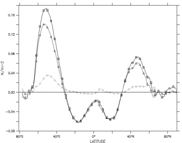
Figure 2 shows the zonal mean of the zonal component of the wind stress for OMIP and ODASI wind products and the
dif-ference between them. We can observe that the zonal wind com-ponent in OMIP is more intense than in ODASI on most latitu-des, especially for the high latitude bands of both hemispheres where the most energetic wind-stress field is found. The diffe-rence between OMIP and ODASI wind-stress globally averaged in space and time is 6.22 × 10¹¹ Watts.day-1 that is of the
same order as the global kinetic energy grow rate (1.82 × 10¹¹
Watts.day-1). It is important to note that the first integration year
is not considered on the kinetic energy growth rate estimate to avoid noises associated with the initial warm-up phase.
Figure 1 – Time series of the integrated ocean kinetic energy for the whole integration domain in PW (PW = 1015W).
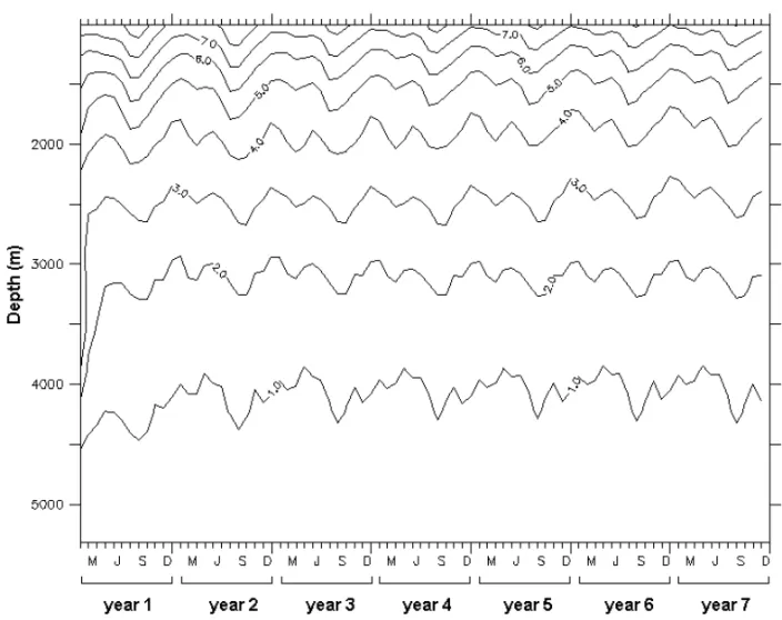
Figure 3 – Time series of ocean kinetic energy integrated for each level between 1000 m and 5500 m for the whole South Atlantic basin (in PW).
The cyclic behavior of the globally integrated kinetic energy was not restricted to the upper layers but also can be seen in deeper ocean layers where the kinetic energy peaks are much less intense. On Figure 3, we plot the ocean kinetic energy integra-ted for each level between 1000 m and 5500 m for the whole South Atlantic basin.
Volume transport analysis
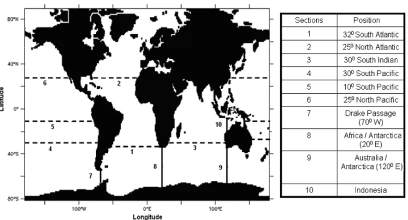
To analyze the model response to the imposed forcing the world ocean was divided in nine sections (three meridional and six zonal), where volume and heat transports were estimated (Fig. 4). In order to allow a comparison with previous works, we chose a set of sections following closely the ones used by Gana-chaud & Wunsch (2000) and Maltrud & McClean (2003). Sec-tion transports were integrated in three different vertical layers: 0-1500 m (upper layer), 1500-3500 m (deep layer) and 3500-5500 m (bottom layer) according to the classification by Maltrud & McClean (2003).
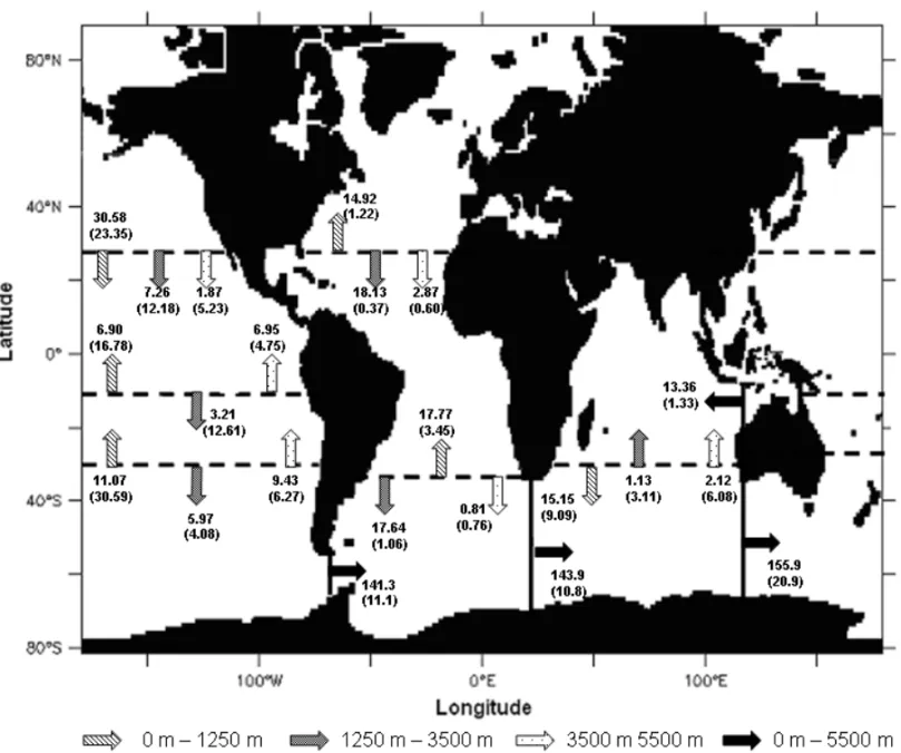
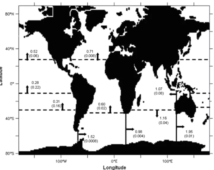
Figure 5 displays the annual mean (for the last six years of integration) of the vertically integrated volume transport (inten-sity and direction) and associated variance across each monitored
section (Fig. 4) in three different levels 0-1250 m (upper layer), 1250-3500 m (deep layer) and 3500-5500 m (bottom layer) for sections 1-6, and in the whole water column for sections 7-9.
The zonal sections situated in the Atlantic Ocean (sections 1 and 2) present similar behavior with a northward volume trans-port for the upper layer and a southward transtrans-port for the deep layers. These results are in accordance with the general ocean circulation in Atlantic sector where heat is exported to the North in the upper layers and to the South by the deep water move-ment. The obtained values agree with literature estimates. Ap-plying an inverse calculation method on WOCE hydrographic data, Ganachaud & Wunsch (2000) obtain 16 ± 3 Sv (1 Sv = 106m3.s-1) and 16 ± 2 Sv northward volume transports in the
upper layer for sections 1 and 2 respectively. Using an eddy resolving OGCM, Maltrud & McClean (2003) find average vo-lume transports of 15 Sv and 16 Sv in the upper layer of the same sections. For the deep layer we get southward transports of 17.64 ± 1.06 Sv and 18.13 ± 0.13 Sv for sections 1 and 2 res-pectively. Schmitz (1996) find southward transports of 18 Sv for both sections while Maltrud & McClean (2003) find 17 Sv and 19 Sv. In section 1, at bottom layer, we find southward
Figure 4 – Sections where volume and heat transports are estimated. Each section is identified by a number and a name.
volume transport. This result does not agree with estimates ob-tained by Schmitz (1996), Ganachaud & Wunsch (2000) and Maltrud & McClean (2003) that found northward transport. This discrepancy is due to the positioning of North Atlantic Deep Water flow at this section whose lower bound is at deeper levels (dee-per than 3500 m). Also, the northward flow of Antarctic Bottom Water, with upper salinity and temperature values of 34.7 and 0.3◦C in this region (Pickard & Emery, 1990), occupies depths
deeper than 3700 m and it is confined to the western side of the basin. If we consider the upper limit of the bottom layer at 3800 m, we estimate a northward volume transport of 1.17 ± 0.41 Sv in this layer, what is comparable with the literature.
In section 2 it is also observed southward transport of 2.87 ± 0.6 Sv. In this section Ganachaud & Wunsch (2000) found also southward transport of 4 ± 2 Sv.
The grid used in the present experiment has a free com-munication between North Atlantic and Arctic Oceans and, con-sequently, ensures the existence of non-zero resultant volume transports. In Figure 6, two zonal and one meridional section situated between Europe and Groveland show the existence of inflows at high latitudes of the North Atlantic. The values have the same order of the ones obtained by Stammer et al. (2003) on close sections. These transports could explain non zero net volume transports through the monitored Atlantic Ocean areas.
In section 3, at the upper layer, our model gives a southward transport of 15.15 ± 9.09 Sv. This value agrees with Schmitz (1996) and Maltrud & McClean (2003) that find 18 Sv and 16 Sv, respectively. The northward deep layer transport presents much less intensity (1.13 Sv) and stronger variability (± 3.11) than the bottom layer values. Ganachaud & Wunsch (2000) also find northward volume transport of 3 ± 5 Sv in this layer on a close section.
The zonal Pacific sections (4 and 5) present northward up-per layer volume transports of 11.07 ± 30.59 Sv and 6.9 ± 16.78 Sv. Section 6 presents southward volume transports for all the monitored layers.
The Indonesian throughflow (Fig. 1, section 10) presents 13.36 ± 1.33 Sv westward volume transport for the whole water column. Ganachaud & Wunsch (2000), Maltrud & Mc-Clean (2003), and Stammer et al. (2003) find for this section: 15 ± 5 Sv, 12 Sv, and 11.5 ± 5 Sv, respectively (Fig. 5).
Figure 5 also shows that the most intense transports are as-sociated with the ACC zonal flux. Due to ACC barotropic nature on its meridional sections (Fig. 4; sections 7, 8, and 9) we cal-culate the volume transports integrated on the whole water. Sig-nificant transport variances are found on these sections proba-bly related with strong OMIP zonal wind stress variance on the ACC zonal band.
Figure 5 – Annual mean (for the last six years of integration) integrated volume transport (direction and intensity) and associated variance (in Sv) for each section
in Figure 2 at three different levels: upper layer (0 m–1250 m), deep layer (1500 m–3500 m) and bottom layer (3500 m–5500 m). It is also plotted some integrated volume transports for the whole water column (0 m–5500 m).
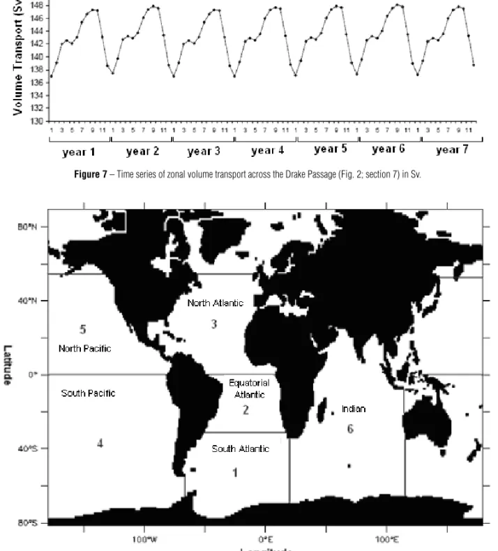
The time series plots of the vertically integrated eastward volume transport of the ACC at Drake Passage (Fig. 4, sec-tion 7) has an annual cyclic behavior with maximum values on austral winter and minimum values on austral summer (Fig. 7). The magnitude of this transport ranges from 137 Sv to 148 Sv. The mean zonal volume transport across the Drake Passage is 143.1 ± 11.1 Sv, which is close to Whitworth & Peterson (1985) estimate of 124.7 ± 9.9 Sv based on multi-years bottom pressure and current meter moorings records. These authors also find the same annual cycle obtained. Based on inverse methods applied to WOCE hydrographic data, Rintoul (1991) find 130 ± 13 Sv, while Ganachaud & Wunsch (2000) find 140 ± 6 Sv.
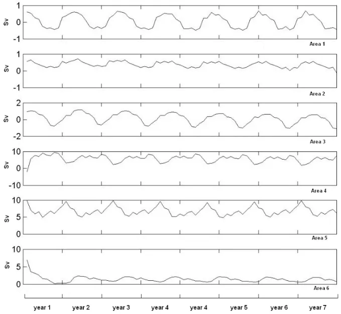
In order to make a volume balance, the world ocean was divi-ded in six different areas (Fig. 8).
On Table 1 we present the average balance of volume inside each monitored area on Figure 8, what help us to evaluate the model ability to produce results that converge to an ocean climate state (Table 1). These values should be analyzed together with the boundary values related with the hydrological cycle used in the model. In this experiment the hydrological cycle was repre-sented by the following variables (in m.s-1): Precipitation minus
evaporation, and runoff. The balance of volume (in m3.s-1) in each
region is divided by the respective area in order to allow a com-parison with hydrological variables that are expressed in m.s-1.
As seen before, the annual mean values related with the balance of volume in each monitored area are insignificant when compa-red with the hydrological cycle variables and would represent an insignificant sea surface elevation growth.
Table 1 – Annual mean values of precipitation minus evaporation balance (PME), land runoff (runoff) and volume transport balance for each
monitored area. Values of PME, runoff and volume transport balance are in m/s (Assad, 2006).
PME Volume transport Total
Area PME Runoff + balance (m3/s) balance
Runoff (variance) (m/s)
South Atlantic –1.25 × 10⁻⁸ 6.4 ×10⁻¹⁰ –1.18 × 10⁻⁸ –1.66 × 10⁻⁹(± 1 × 10⁻⁸) –1.35 × 10⁻²⁰
Equatorial Atlantic –1.86 × 10⁻⁸ 5.6 × 10⁻⁹ –1.29 × 10⁻⁸ 1.03 × 10⁻⁸(± 5 × 10⁻¹⁰) –2.6 × 10⁻²¹
North Atlantic 1.62 × 10⁻⁸ 2.49 × 10⁻⁸ 4.1 × 10⁻⁸ 2.1e-9(± 6.7 × 10⁻⁹) 4.31 × 10⁻²⁰
South Pacific –2.22 × 10⁻⁹ 1.03 × 10⁻⁹ –1.19 × 10⁻⁹ 4.3 × 10⁻⁸(± 3.2 × 10⁻⁸) –4.19 × 10⁻²⁰
North Pacific 8.13 × 10⁻⁸ 2.54 × 10⁻⁸ 1.06e-7 1.22e-7(± 3 × 10⁻⁸) 2.28 × 10⁻²¹
Indian 1.54 × 10⁻¹⁰ 2.32 × 10⁻⁹ 2.47 × 10⁻⁹ 1.37 × 10⁻⁸(± 7 × 10⁻⁹) 1.51 × 10⁻²¹
Figure 6 – Annual mean volume transports (in Sv) and associated variance across the sections localized between North America, Groveland and Europe.
In Figure 9 it is shown a time series plot of the volume trans-port balance for each monitored area. It is possible to observe a well defined cyclical behavior in all monitored areas.
Heat transport analysis
Before we start, it is important to emphasize that what we call “heat transport” in this section is, in fact, the heat advection (advective heat transport).
In Figure 10, we plot the mean vertically integrated (from surface to bottom) heat transport and respective variance across
each monitored section (Fig. 4). The Atlantic and Pacific zonal sections (Fig. 4; sections 1, 2, 4, 5, and 6) present northward heat transports, while the Indian Ocean zonal section (Section 3) presents a southward heat transport that agrees with other estima-tes (Ganachaud & Wunsch, 2000; Stammer et al., 2003).
Section 1 presents a northward heat transport of 0.60 ± 0.02 PW (1 PW = 1015 Watts), what reinforces the peculiar
be-havior of the South Atlantic basin as exporter of heat to the North Atlantic. The same behavior is observed across section 2, but with an enhanced northward heat transport that could be
Figure 7 – Time series of zonal volume transport across the Drake Passage (Fig. 2; section 7) in Sv.
Figure 8 – Ocean areas defined to analyze the balance of heat and mass.
associated with the strong upper layer (0-1500m) northward heat and volume transports associated with the Gulf Stream. North-ward resultant heat transports were also observed in the works of Ganachaud & Wunsch (2000) and Stammer et al. (2003) at close sections.
The most intense heat transports are associated with the ACC zonal flux through its meridional sections (Fig. 4; sections 7, 8, and 9). The time series plot for the vertically integrated heat transport perpendicular to each monitored section also reveals a
well defined annual cycle behavior (not shown). For the Drake Passage section (Fig. 4; section 7), maximum values are found during austral summer and minimum during austral winter (Fig. 11). The magnitude of this transport ranges from 1.48 to 1.58 PW with a mean value of 1.52 ± 0.0008 PW. These values agree with previous estimate of 1.3 PW by Ganachaud & Wunsch (2000).
Another significant westward heat transport is observed in Indonesia meridional section (Fig. 4; section 10). In this section it is estimated an annual mean value of 1.07 PW ± 0.08 PW.
Figure 9 – Time series of volume transport balance (in Sv) for each monitored area exposed in Figure 8.
Stammer et al. (2003) find an westward heat transport of 1.12 PW ± 0.52 PW from an ocean general circulation model and Gana-chaud & Wunsch (2000) find 1.4 PW westward heat transport by the application of inverse methods.
Table 2 – Annual mean resultant heat flux on ocean surface (in PW)
integrated in each monitored area. Positive values indicate ocean heat gain and negative values ocean heat loss (Assad, 2006).
Area Ocean surface resultant heat flux (PW) South Atlantic 0.93 (± 4.21) Equatorial Atlantic 1.12 (± 0.75) North Atlantic –1.90 (± 3.62) South Pacific 3.93 (± 34.7) North Pacific –2.32 (± 9.78) Indian 1.76 (± 9.27)
Table 2 shows the gain (positive values) or loss (negative va-lues) of heat by each monitored ocean area shown in Figure 8. It reveals a net gain of heat by southern hemisphere ocean surface and a net loss of heat by the northern hemisphere ocean surface. Figure 12 reveals the presence of an intense northward heat transport between equator and 40◦N and a southward heat
trans-port between the equator and 40◦S what indicates that the
con-ducted experiment was able to reproduce the so-called conveyor belt circulation. Using a geostrophic method on data obtained during the WOCE project, Ganachaud & Wunsch (2000) esti-mate the mean value of –0.6 ± 0.3 PW for the global meridional heat transport across 30◦S and 2.2 ± 0.6 PW on 12◦N. On the
same latitudes we find –0.2 ± 0.01 PW and 1.75 ± 0.03 PW, respectively.
The heat transport analysis also reveals a well defined cy-cle for this property. Again, it is also possible to see a small
Figure 10 – Annual mean vertically integrated heat transport (direction and intensity) and associated variance (in PW) for each section in Figure 2.
Figure 11 – Time series of zonal heat transport (in PW) across the Drake Passage (Fig. 2; Section 2).
growth tendency that could be related with the imposition of the new heat flux boundary condition to the model. The ODASI uses initial conditions generated by a numerical experiment where sea surface temperature data assimilation techniques were applied. As presented before, the heat flux boundary conditions used in this experiment are the climatological OMIP data. In Table 2,
it is presented the resultant sea surface heat flux integrated in each monitored area. Positive values are found on Southern Hemisphere, what demonstrate the importance of these oceans as heat reservoirs of the Earth’s climate system. In contrast, Northern Hemisphere ocean present negative surface heat flu-xes. This fact can be related with the ratio of land/ocean area
Figure 12 – Global integrated annual mean meridional heat transport (in PW).
that is almost three times bigger on Northern Hemisphere than on the Southern Hemisphere (Peixoto & Oort, 1992). Another im-portant point to emphasize is the high variance values associa-ted with each sea surface heat flux estimate, especially on equa-torial regions. This fact could be associated with surface veloci-ties that are strong influenced by wind field fluctuations that are very significant on this region.
CONCLUSIONS
The estimated annual mean volume and advective heat transports across the sections in Figure 4 agree with existing in literature. It can be observed some significant variances associated with meridional transports in low latitude regions, especially, in up-per levels due to strong wind spatial and temporal variations in these regions. The ACC volume transport at Drake Passage re-veals a well defined seasonal cycle starting at the second inte-gration year and followed the same seasonal behavior found in the scientific literature. Also, high ACC volume transport varian-ces are found, what seems to be related with barotropic fluctuati-ons of the OMIP zonal wind-stress variance on that latitude band. Some important physical aspects of the ocean global circulation,
as the so-called conveyor-belt meridional heat circulation, could also be observed on model results. The northward advective heat transport found in the 32◦South Atlantic section is in accordance
with the scientific literature.
The initialization strategy used on the present work was suc-cessful in decreasing the model spin-up time. This work shows that the chosen model configuration and initialization strategy is able to reproduce the main balances in the world oceans, what ma-kes this model suitable for longer integration periods for studying low frequency climate events. The obtained results could consti-tute an important data source to be used as initial and boundary conditions in regional ocean model experiments, as well as, for long integration runs in order to study oceanic climate variability.
ACKNOWLEDGEMENTS
The authors would like to thank the ocean and climate group of GFDL for the strong help in configuring the ocean model and tur-ning available the needed data to initialize the experiment. The third author would also like to thank the National Council for Scientific and Technological Development (CNPq) for the sup-port under VARICONF project (Grant #476472/2006-7).
REFERENCES
ASSAD LPF. 2006. Influˆencia do Campo de Vento anˆomalo tipo ENSO na Dinˆamica do Atlˆantico Sul. Doctorate Thesis, Universidade Federal do Rio de Janeiro, Rio de Janeiro, 222 p.
BRYAN K & LEWIS LJ. 1979. A water mass model of the world ocean. Journal of Geophysical Research, 84: 2503–2517.
GANACHAUD A & WUNSCH C. 2000. Improved estimates of global cir-culation, heat transport and mixing from hydrographic data. Nature, 408: 453–457.
GRIFFIES SM, GNANADESIKAN A, DIXON KW, DUNNE JP, GERDES R, HARRISON MJ, ROSATI A, RUSSELL JL, SAMUELS BL, SPELMAN MJ, WINTON M & ZHANG R. 2005. Formulation of an ocean model for global climate simulations. Ocean Science, 1: 45–79.
JAKOBSSEN M, CHERKIS N, WOODWARD J, MacNAB R & COAKLEY B. 2000. New grid of Arctic bathymetry aids scientists and mapmakers, EOS Trans. Am. Geophys. Union, p. 81, 89, 93, 96.
LARGE WG, McWILLIAMS JC & DONEY SC. 1994. Oceanic vertical mi-xing: A review and a model with non-local boundary layer parameteriza-tion. Rev. Geophys., 32: 363–403.
LARGE WG, DANABASOGLU G, McWILLIAMS JC, GENT PR & BRYAN FO. 2001. Equatorial circulation of a global ocean climate model with anisotropic horizontal viscosity. Journal of Physical Oceanography, 31: 518–536.
LEVITUS S. 1982. Climatological Atlas of the World Ocean. – NOAA Prof. Pap. No. 13. U.S. Government Printing Office, Washington, DC, 173 pp.
MALTRUD ME & McCLEAN JL. 2003. An eddy resolving global 1/10◦
ocean simulation. Ocean Modelling, 8: 31–54.
MATANO RP & PHILANDER SGH. 1993. Heat and Mass Balances of the South Atlantic Ocean calculated from a Numerical Model. Journal of Geophysical Research, 98: 977–984.
MOREL A & ANTOINE D. 1994. Heating rate within the upper ocean in relation to its bio-optical state. Journal of Physical Oceanography, 24: 1652–1665.
MURRAY RJ. 1996. Explicit generation of orthogonal grids for ocean models. Journal of Computational Physics, 126: 251–273.
OORT AH, ANDERSON LA & PEIXOTO JP. 1994. Estimates of the energy cycle of the oceans. Journal of Geophysical Research, 99: 7665–7688.
PACANOWSKY RC & GRIFFIES SM. 1999. The MOM3 Manual. Geophy-sical Fluid Dynamics Laboratory/NOAA, Princeton, USA, p. 680. PEIXOTO JP & OORT AH. 1992. Physics of Climate. American Institute of Physics. 520 pp.
PICKARD GL & EMERY WJ. 1990. Descriptive Physical Oceanography: An Introduction. Pergamon Press. 320 pp.
RINTOUL SR. 1991. South Atlantic Interbasin Exchange. Journal of Geophysical Research, 96: 2675–2692.
R¨OESKE F. 2001. An Atlas of Surface Fluxes based on the ECMWF Re-Analysis – a Climatological Dataset to force Global Ocean General Circu-lation Models. Max-Planck Institut f¨ur Meteorologie, Hamburg. Report no. 323. ISSN 0937–1060.
SCHMITZ WJ. 1996. On The World Ocean Circulation: Volume II. Te-chnical Report. Woods Hole Oceanographic Institution. WHOI-96-08. 241 p.
SEMTNER AJ & CHERVIN RM. 1992. Ocean General Circulation from Global Eddy-Resolving Model. Journal of Geophysical Research, 97: 5493–5550.
SMAGORINSKY J. 1963. General Circulation experiments with the pri-mitive equations I. The basic experiment. Monthly Weather Review, 91(3): 99–164.
SMITH WHF & SANDWELL DT. 1997. Global sea floor topography from satellite altimetry and ship depth soundings. Science, 277: 1956–1961. STAMMER D, WUNSCH C, GIERING R, ECKERT C, HEIMBACH P, MAROTZKE J, ADCROFT A, HILL CN & MARSHALL J. 2003. Volume, heat, and freshwater transports of the global ocean circulation 1993-2000, estimated from a general circulation model constrained by World Ocean circulation Experiment (WOCE) data. Journal of Geophysical Re-search, 108: pp. 7-1–7-23.
SUN C, RIENECKER MM, ROSATI A, HARRISON M, WITTENBERG A, KEPPENNE CL, JACOB JP & KOVACH RM. 2007. Comparison and Sen-sitivity of ODASI Ocean Analyses in the Tropical Pacific. Monthly Weather Review, 135: 2242–2264.
WHITWORTH T III & PETERSON RG. 1985. The volume transport of the Antarctic Circumpolar Current from bottom pressure measurements. Journal of Physical Oceanography, 15: 810–816.
WUNSCH C. 1998. The work done by the wind on the oceanic general circulation. Journal of Physical Oceanography, 28: 2332–2340.
NOTES ABOUT THE AUTHORS
Luiz Paulo de Freitas Assad. Bachelor in Oceanography (UERJ/1996), Master in Physical Oceanography (USP/2000) and Doctor in Civil Engineering in the
area of computational modeling applied to the Environmental Engineering (UFRJ/2006). At present, he is researcher at COPPE/UFRJ. His area of interest is Physical Oceanography, with emphasis in ocean computational modeling, acting mainly in the following subjects: global and regional ocean computational modeling, ocean climate variability, and analysis of oceanographic data.
Audalio Rebelo Torres Junior. Bachelor in Meteorology (UFRJ/1982), specialized in Signal Processing Neural Networks (Petrobras/1992), Master in Oceanic
Engineering (UFRJ/1995), and Doctor in Oceanic Engineering (UFRJ/2005). At present, he is professor at the Meteorology Department/UFRJ. The Physical Oceanography is his area of interest, working mainly in the following subjects: El Ni˜no, ocean circulation, climate, numerical modeling, teleconnections processes, and oceanography of the South Atlantic.
Wilton Zumpichiatti Arruda. Bachelor in Computer Science (UFRJ/1990), Master and Doctor in Mathematics (UFRJ/1991, 1996), and Ph.D. in Physical
Oceano-graphy at Florida State University (2002). He is professor at Mathematical Institute/UFRJ since 1995. His areas of interest are: ocean circulation, ocean modeling, climate changes, and remote sensing among others.
Affonso da Silveira Mascarenhas Junior. Bachelor in Physics (USP/1967), Master in Meteorology (INPE/1976), Master in Physical Oceanography at the
Mas-sachusetts Institute of Technology (1979), and Ph.D. in Physical Oceanography at the MasMas-sachusetts Institute of Technology (1981). Professor at USP (1972-1993), Universidad Aut´onoma de Baja California (1993-2008), and nowadays he is director of the International Centre of Investigation on the El Ni˜no Phenomenon. His areas of interest are: observational and synoptical physical oceanography, sea meteorology, and remote sensing.
Luiz Landau. Bachelor in Civil Engineering (PUC-RJ/1973), Master in Civil Engineering (UFRJ/1976), and Doctor of Civil Engineering (UFRJ/1983). At present, he is
professor at UFRJ. His area of interest is Civil Engineering, with emphasis in structures, working mainly in the following subjects: finite elements methods, computational methods, oil producing systems, virtual reality, and biomarkers.