THE WORLDWID IMPACT OF INSTITUTIONAL FUNDS ON
FLOW-PERFORMANCE RELATIONSHIP
DAN SU
Dissertation submitted as partial requirement for the conferral of Master in Finance
Supervisor:
Prof. António Manuel Freitas Miguel, ISCTE Business School, Department of Finance,
Thesis License Agreement
Name:
E-mail: email Phone number: Phone
Identity Card/Passaport: number
Nationality: nationality
Master's (Dissertation) ☐ Master's (Project) ☐
Title of the Dissertation / Project:
Title
Supervisor (s): Supervisor name Conclusion Year: 2016
Master course designation: Master in
I declare under oath that the dissertation/project now delivered is the final version. Otherwise, it will be later presented the version that the jury has approved.
I grant to ISCTE-IUL and its agents a non-exclusive license to archive and make accessible, through its institutional repository in the conditions below, my dissertation or project, in whole or in part, in digital format:
☐ Immediate availability of work set for worldwide access;
☐ Availability of work set for exclusive access in ISCTE-IUL during the period of ☐ 1 year, ☐2 years or ☐ 3 years, and after the time appointed I authorize worldwide access. ☐ Availability of work set for exclusive access in ISCTE-IUL.
☐Embargo (Granted in exceptional circumstances by justified reason. Failure to provide documentation in support of the request, invalidate the same).
I hold all copyright of the dissertation or project and the right to use in future works (such as articles or books).
ISCTE-IUL, Signature date Signature:
Declaration of Honour Dissertation delivery / master's Project Work
I, the undersigned, hereby declare:
I am the exclusive author of the presented work, my work is original, and I used references and quoted all sources used.
I authorize that my work be submitted to SafeAssign - plagiarism detection tool. I am aware that the practice of plagiarism, self-plagiarism and copying is an academic illicit.
Full Name
Master Student Number
ISCTE-IUL e-mail address
Personal email address
Phone contact
ISCTE-IUL ,2017
1
Honorable Rector of the ISCTE-IUL,
I, having completed all
courses of the Master in , I hereby
request permission to submit dissertation / master's project work.
Requests approval,
(Place), , 2017
2
Abstract:
This thesis uses data from 15 countries, over the 1998-2010 period, to examine and compare differences in the flow-performance sensitivity between institutional and retail investors. Our results show that the flow-performance relationship is convex, consistent with previous research, but the impact of institutional funds on flow-performance relationship outside the US is marked different from the US. Compared to retail investors, institutional funds sell more poor performance funds and buy less top performance funds outside the US while institutional investor act the same way as retail investors to past performance in the US. We then split our sample into more and less sophisticated countries, investors buy more top performers but only in less sophisticated countries. When it comes to bottom performance, the reactions are similar for both more sophisticated and less sophisticated countries. Our finds provide evidence that institutional investors are more sophisticated than retail investors in less sophisticated countries and retail investors are sophisticated as institutional investors in more sophisticated countries, like the US.
Keywords: Mutual funds, Flow-performance relationship, Convexity, institutional
investors, Investor sophistication
3
Resumo
Esta tese usa dados de 15 países, durante o período 1998-2010, para examinar e comparar as diferenças na sensibilidade dos fluxos monetários à performance entre investidores institucionais e investidores retalhistas. Os resultados mostram que a relação fluxo-performance é convexo, consistente com a literatura, mas o impacto dos fundos institucionais nesta relação nos EUA é marcadamente diferente da que existe noutros países. Em comparação com os investidores retalhistas, os investidores institucionais vendem mais fundos com desempenho baixo e compram menos fundos com elevado desempenho fora dos EUA, enquanto não há diferença entre investidores institucionais e retalhistas nos EUA. Em seguida, dividimos nossa amostra em países mais e menos sofisticados. Os investidores compram mais fundos com elevado desempenho, mas apenas em países menos sofisticados. Quando se trata de fundos com desempenho inferior, as reações são semelhantes para países mais sofisticados e menos sofisticados. Os nossos resultados permitem concluir que os investidores institucionais são mais sofisticados do que investidores retalhistas em países menos sofisticados e o nível de sofisticação é semelhante nos países mais sofisticados, como os EUA.
Palavras-chave: Fundos de investimento, Relação fluxo monetário-desempenho, Convexidade, Investidores institucionais, Sofisticação do investidor
4
Acknowledgements
First of all, I would like to express my appreciation to my supervisor, Prof. António Freitas Miguel for his patient and expert guidance. Thanks a lot for all the helpful suggestions and support especially on the data construction with STATA. I am very grateful to have such a responsible and inspiring supervisor. Moreover, I thank my friends in Lisbon a lot for them accompanies and supports. Thank them bring so much smiles and happiness in my master and give me courage to try something new. Finally, I appreciate all the encouragement and selfless support from my family.
5 Index of content Abstract: ... 2 Resumo ... 3 Acknowledgements ... 4 Index of content ... 5
Index of figure and tables ... 6
1.Introduction ... 7
2. Literature review ... 11
3. Sample and variables construction ... 22
3.1 Sample description ... 22 3.2 Variables construction ... 26 3.2.1 Fund flows ... 26 3.2.2 Performance measurement ... 28 3.2.3 Control variables ... 33 4. Methodology ... 34
4.1 The flow-performance sensitivity ... 34
4.2 The flow-performance relationship with institutional funds ... 36
5. Results ... 37
6. Explaining the flow-performance relationship across countries ... 43
7. Conclusion ... 47
6
Index of figure and tables
Table 1. Number of funds and total net asset for all sample ... 24
Panel A: numbers of funds and total net asset (TNA) for all samples by country ... 24
Panel B: Number of funds with institutional funds by country ... 25
Table 2. Descriptive statistics of fund flows by country across all funds, institutional funds and retail funds ... 27
Table 3 fund variables ... 31
Panel A. Fund-level variables averaged across fund quarter by country ... 31
Panel B. Pairwise correlation of fund-level variables ... 32
Table 4 The impact of institutional funds on flow-performance relationship ... 38
Panel A: The flow-performance measured by linear regression ... 38
Panel B: The flow-performance measured using three pieces model ... 41
Table 5: Country-level proxies for investor sophistication ... 44
Table 6: Flow-performance sensitivity and country-level investors sophistication ... 46
Appendix: The one-factor model of flow-performance relationship ... 52
Panel A: The flow-performance measured by linear regression ... 52
7
1.Introduction
In this study, we testify and compare the form of flow-performance relationship for institutional and retail mutual funds.
The interest of this paper stems from three strands resources. First, most literature measures the relation between fund inflows or outflow and last returns and conject that the flow-performance relationship is convex. Chevalier and Ellison, (1997) show that investors in mutual fund wish the maximization of risk-adjusted return while mutual fund manager only alter risk for attracting more flows according to last performance. Sirri and Tufano, (1998) find mutual fund investors flock disproportionately more assets to winners but fail to invest aptly to losers. Berk Green (2004) argue that the flow-performance relationship could consider to be determinant to reflect the average skilled level of the managers. Ferreira, Keswani, Miguel, and Ramos (2012) compare the flow-performance relationship across countries and conclude that this relationship has a more concave form in developing countries with less developed mutual fund industries ans less sophisticated investors, while the relationship is less convex in more developed countries, i.e., countries with more developed economies, and where the financial markets and the mutual fund industries are more developed. The paper also explains these findings with the fact that investors in developed countries are more sophistication and face less participation costs.
The second strand of literature highlights that the way that flows respond to past returns, indicates persistence of mutual fund performance. (for example, Goetzmann and Peles ,1997; Carhart, 1997; Huang, Wei, and Yang ,2007; Kosowski,
8 Timmermann, Wermers and White, H., 2006). Studies on performance persistence are measured by risk-adjusted return, as absolute return are prone to bias risk with sample error. Ivković and Weisbenner (2008) provide evidence that purchase decisions rely on risk-adjusted return, providing predictive information of future performance, while sale decisions focus on the past absolute performance and the relevant tax benchmarks. Further, studies show that returns are generally persistent at the top and bottom level of performance. Elton and Gruber (1996) find that top performance funds continue to perform well but bottom performance funds continue to generate inferior returns. Finally, different studies show that fund flow persist in both outperformers and underperformers, as well. Chevalier and Ellison (1997) and Del Guercio and Tkac (2002) point out the “herding effect”, which attract inflows into funds that perform well and widraw assets from poor performers.
Additionally, one third strand of research compares the differences between institutional and non-institutional funds, including, Berger (1997), James and Karceski (2006), Knack (1995) and others. Consistent with different nature of investors, studies on this area focus on the differences of flows toward these two types of funds. Salganik-Shoshan (2016), compares retail and institutional investors, and find that institutional investors are more sensitive to quantitative performance measures while evaluating funds. Moreover, previous empirical findings show that there is a non-linear flow-performance relationship for both retail and institutional mutual fund in the US (see, e.g., Karceski , 2002; and Mazur, 2017).
9 argue that, in countries where the financial markets and the mutual fund industry is more developed - like in the U.S., the country with the oldest and the most developed mutual fund industry in the world (Ferreira et al., 2012) - institutional and retail investors are both expected to respond to past performance the same way. This is because the level of sophistication of retail and institutional investors is expected to be similar.. In countries with less developed financial markets, and less mutual fund industries, however, retail and institutional fund flows may react differently to past performance. In this countries, investors are less sophisticated (see, e.g., Ferreira et al.,2012) and therefore we would expect retail investors to be on average less sophisticated than institutional investors. We also expect the flow-performance relationship to bee convex in both the US and outside the US, consistent with previous studies (see, e.g., Huang, et al., 2007). Finally, we expect investors in more sophisticated countries to be able to deal with information more rationally. For these conjectures, institutional funds are more likely sophisticated than retail funds and we expect the impact of institutional funds on flows corresponding to last returns has a more convex relationship in less developed countries. Consistent with Ferreira et al. (2012), investor sophistication is expected to affect more the top range of the flow-performance relationship. To examine these issues, we use a large sample of actively equity mutual funds, including 15 countries during the period from 1998 to 2010. The sample integrates over 27,000 equity funds and $12 trillion total net assets.
We find that the response of institutional investors to flows is different when we compare the U.S. with non-US countries, meaning that the results for the U.S. are
10 unsuitable to represent all other countries. The results show that institutional investors buy less winners and sell more losers only outside the US. We hypothesize that investor sophistication, explains the differences on how retail and institutional investors react to past performance across countries. We rank the performance into low, mid and high performance and, when we compare how institutional investors respond to top performance, we find that they are more sensitive to past performance in more sophisticated countries. When it comes to bottom performance, we find that the reactions are similar for both more sophisticated and less sophisticated countries. Our findings provide evidence for the view that institutional investors are more sophistication than retail investors in less sophisticated countries and retail investors have the same degree of sophistication as institutional investors in more sophisticated countries, like the US.
Our study makes several contributes to mutual-fund literature. First, our empirical results of flow-performance relationship for all funds, the US and non-US countries provide heterogeneity evidence for previous researches. Second, our study is the first one to testify the link between institutional fund flows and past performance with a worldwide sample. There is no study on institutional funds across countries, while most existed across-countries researches are focus on participant cost (Khorana et al., 2008), flows (Ferreira et al., 2012) and performance (Keswani et al., 2016). Finally, we shed light on the impact of investor sophistication on the flow-performance relationship contributing to explain the differences between in the US and outside the US.
11 The remainder of this paper is structured as follows. The next section presents literature review. Section 3 describes the dataset of our sample and variables constructed to measure the sensitivity of fund flows and performance. Section 4 outlines the methodology. Section 5 reports the results of our analysis. Section 6 examines the role of sophistication in the flow-performance relationship. Section7 concludes.
2. Literature review
Numerous papers compare the retail and institutional funds through each respect like flow- performance, investor behavior and portfolio choice. These papers mostly investigate the US equity fund market and find that the differences in the flow-performance relationship of between retail and institutional investors are not significant.
Salganik-Shoshan, (2016) investigates U.S. equity mutual funds from 1999 to 2012. After comparing the fund criteria used by investors, the results show that retail investors are less sophisticated than institutional investors, whose flows are more sensitive to sophisticated adjusted performance criteria, such as Jensen’s alpha, risk-adjusted return measures and tracking error. Both retail and institutional investors prefer lower expense and “smart money”, allocating more assets into past best-performance. But herding behavior is stronger in institutional mutual fund.
Karceski (2002) studies the portfolio choice and investment behavior distinguishing between retail investors and institutional mutual fund investors. By
12 comparing the flows and performance into institutional and non-institutional funds, they find that institutional funds do not chase more returns than retail funds. Also there is no significant relation of flow and performance among institutional funds, but a positive relationship for retail funds. For top performance, institutional investors are significantly less sensitive to inflows than retail investors. Although flows for both types of funds are significantly related to the level of fees charged, retail investors flows are more sensitive. Splitting the institutional funds based on minimum investment requirements, they find that low requirement institutional funds and institutional funds mates with retail funds underperform more than retail funds. High expenses, low sensitivity of flows and lower returns are hard to explain the bad performance of small institutional funds.
Mazur (2017) studies the relationship of flow and performance for the US institutional and retail mutual funds. The results confirm that the both US retail and institutional investors react to the flow-performance relationship similarly. Further, institutional investors are sensitive to adjusted-return measures whereas retail investors concentrate on absolute returns. However, by splitting the performance into top and bottom performers, they find that retail investors transfer their assets from losers to winners for punishing underperformers, while institutional investor prefer to divest from bottom performance. These findings infer that institutional funds are more consistent with concavity while retail investors mainly attribute to convexity.
Berger (1997) investigates the efficiency of the financial institutions. Each corresponding measurement to the relation between past performance and their
13 efficiency is reasonable but different. In this paper, the efficiency is explained with economic concepts. Through the examination, various measurement techniques present similar robust results about the efficiency. Substantial unexploited data of economic scale costs in the 1990s is found, suggesting that larger banks haves advantage of the technology and risk tolerance. The regressions models show that the complications and the inefficiencies in the mutual fund industry are quite huge, around 20% which is more than the average inefficiency for banking industry and beats the potential profits of the industry. As well, the explanation about the efficiency is still a huge task in the future, reconfirming the previous literatures. Th vast majority of previous studies examining he determinants of funds flows are linked to past returns and find that the flow-performance is convex.
Ferreira et al. (2012) concludes that the US finding from previous researches are not consistent with other countries as there are significant differences from the link between flow and performance. Through examining the flow-performance relationship from individual countries, the results show that investors in more developed countries sell more underperformers and buy less top performers. The paper explains these phenomenon with investor sophistication and participation costs, which are proxied by economic, financial and mutual fund industry development variables. The results show that more developed countries have more sophisticated mutual fund markets with less risk tolerance, and more sophisticated investors and less participation costs, are consistent with a less convexity. Hence, sophisticated investors sell more losers and buy less winners.
14 Del Guercio and Tkac (2002) shows that the flow-performance relation in retail mutual funds and fiduciary pension funds is quite similar but still some differences exist, as the fundamental operated environments are different. The flows do not react to the performance directly for both types of funds. Although initial excess return seems to be an important factor to flows, the results shows that exceeding the performance of the benchmark index is determinant. To punish the underperformers, both withdraw their assets. In contrast to pension funds, mutual fund clients invest more in past winners and managers alter their portfolio risk to boost their performance. The majority of retail mutual fund investors do not rely on quantitative performance evaluation measures.
Sirri and Tufano, (1998) studies the determinants of inflows and outflows of equity mutual funds. Consumers focus on prior performance information of funds while making decisions, and chase top performance strongly and flee from bottom performance. Investors react to the search costs asymmetrically, as well, preferring lower fees. This paper tries to explain this phenomenon through three aspects. Firstly, the risk-adjusted return with active management should beat passive index funds and funds with higher fees should perform strongly than lower fees, so the funds that perform better attract more investors. Moreover, larger media coverage of mutual fund seems to accelerate the faster cash flow growth even though the best and worst performers are disclosed equally. Finally, a larger mutual fund complex is an important determinant of capital flows, probably because the larger institutional size reduces the cost of consumer research costs.
15 Chevalier and Ellison (1997) show that the flow-performance is affected by investor behavior of both retail investors and managers, and treated as an incentive factor to interpret the behavior of mutual fund companies or managers implicitly. Funds altering the riskiness of the portfolio rely on the flow-performance relationship. Valuating the performance component of Scharfstein ad Stein’s model directly, they find that the herd effect, that drives investors to invest more assets in good performance, is not obvious in mutual fund institution. Also, window-dressing should not serve as a determinant for the quality of fund manager since window dressed could not reward for the retail fund investors.
Berk Green (2004) derive a rational model about active portfolio management which redefines the previous special case into regularities. The relation between flow and performance can reflect the skill level of the fund manager. In this model, the winners are consistent with geometrical age, but the performance of active management is no more than passive index on average. And performance seems to be not persistent while the short-term survival rates could be measured and long-term will renew with time. Furthermore, the flow-performance relationship is determined by prior returns and fees. Finally, this model solves the financial question on how to measure manager skills. Treating the managed fees as the base line, the flow-relationship in some degree can reflect manager skills . The investors prefer to maximize returns with fees, chasing the top performance intensively.
Ivković and Weisbenner (2008) study the relation between the possibility of individuals’ investor sale decisions and fund performance. First, the behavior that the
16 individuals keep winners and sell losers is explained by tax incentives. Tax payments do not only occur when funds are sold or purchased, but also occur due to funds past returns. Thus, investors are sensitive to taxes which is considered as the determinants of the further contributions. Second, the retail investors concentrate on investment costs while deciding to redeem the funds. The redemption expense will increase by the increased proportion of withdrawing assets. Finally, individuals’ sale or purchase decision of the mutual funds are determined by the past performance, but in different ways. Inflows are only sensitive to ‘‘relative’’ performance, suggesting that new money chases the best performers in an objective, while outflows are related only to “absolute’’ fund performance, the relevant benchmark for taxes.
Goetzmann and Peles (1997) show that consistent with Festinger’s psychology hypothesis, the mutual fund investors are inclined to positive past fund performance for reducing the anxiety of purchase decisions. This study investigates the individual’s response to the choice and holding of mutual fund and finds that even though the investors have a positive bias, the economic costs accompanied with the transactions are hard to prevent, which in some extent explains why investors are less sensitive to bottom performance. According for the cross- sectional model, the efficiency of mutual fund information seems to not use correctly the differences between uninformed managers and managers with information are very small. Cognitive dissonance is more important than rational investment in mutual fund industry. For instant, if investors concentrate more on good performance in the past, the optimal mutual fund will drive more demands, that this herd effect forces the fund to increase
17 their quantity and volatility, increase the trade costs as well. The study tries to explain the inertia effect with fund advertisement. The figure displays that the choice of mutual fund relies heavily on investor’s bias, and the advertising could enhance impression but could not affect the choice of investors.
Moreover, many papers study the impact of participant costs or expenses on the flow- performance relationship.
Huang et al (2007) shows a single model to highlight the role of participant costs in the response of mutual fund flows to past performance. By incorporating fund-level participation costs, investors put forward new demand for the growth of capital return and treat the participation costs as baseline or barrier which investors hope to surpass. Through the past returns, the ability of managers is realized; and hence, flows are more sensitive to performance on the effects of participant costs. Moreover, different levels of transaction costs have different sensitivities of flow-performance relationship. The results show that the flow-flow-performance relationship with lower participant costs is consistent with concavity, meaning that lower participant costs are more sensitive of medium performance than other performance rank. High-participant-cost funds are more sensitive to top performance than low-cost counterparts.
Khorana et al. (2008) examine fund fees across developed countries with a database of 18 countries. The study finds that fees are different across countries and even varies from fund to fund, which are relied on the characteristics of the fund types and their fund family. Moreover, fees are related with the number of countries they
18 sold. Fees of on-shore funds with increasing countries sold become smaller while fees are higher in off-shore with an increasing number of countries sold. To explain these variations, the law and other characteristics of funds are considered. The results show that the fees are smaller in those countries with superior judicial systems and higher educations. Also, fees have a significantly negative relation with the age of fund.
Many studies focus on how to measure performance and investigate the relevant variables of measurement.
Gruber (1996) raises a question that “why mutual funds and in actively particular managed mutual funds have grown so fast, when their performance on average has been inferior to that of index funds”. For solving this puzzle, this study examines average performance with raw return and risk-adjusted return, index funds, persistence of performance and predictive cash flows. The risk-adjusted returns earned on new cash flows surpass the return earned by both average active and passive fund. Two hypotheses from results could explain these questions. One possible explanation is that the price of funds is sold and bought equal to net asset value and management ability is non-priced but predictable through past returns or other metrics. Other one is that sophisticated investors attribute to a larger percentage of new cash flows into and out of mutual funds which outperform corresponding benchmarks. The figure provides evidence on investors in actively managed mutual funds who have been more sophisticated than we assume before.
Elton et al. (1996) study the predictability for mutual funds with risk-adjusted returns and show that, in some extent, the information carried in the past predicts the
19 trend of funds returns in the future. Both 1-year and 3-year alphas deliver information about future performance and this information works for 1 year and 3 years period in the future respectively. The alpha variable covers more years, the prior year’s data conveys much more information about the performance. Moreover, applying modern portfolio theory to past returns leads to a positive selection and an optimal portfolio, which performs better than equally weighted portfolio and past rank alone. High expenses have negative impact on future return of the portfolio and the bottom performance always contains majority of funds with high expenses. A smart active funds manager would not increase their fees.
Carhart (1997) explains persistence in equity mutual fund’s risk-adjusted returns with common factors in stock returns and investment expenses. This study focuses on long-term persistence instead of short term. Mostly spread of annual return could be explained by common factors, the rest are strong underperformance. Moreover, this study examines the relation between of performance and skilled or informed mutual fund managers. 4-factor alpha model in this sample demonstrates that higher expected return is relative to high alpha funds, but high alphas could not ensure that the alpha in next quarter is above average and the next return surpasses the market. Finally, the results show that “hot hand” effect are driven by one-year momentum effect without trade costs.
The literature also shows find that fund flows are also sensitive to fund size and family size. Brown (2012) presents a model to evaluate the skill of mutual funds based on both its own last performance and its family’s performance, as previous
20 literature find that the resources of family could produce unobservable return across funds in the same family. To measure the impact of family funds, this paper highlights the potential effects of one fund’s performance on another fund’s returns in the same fund family. “common-skill joint effect” exists between member funds and family funds, but it possibly includes some good luck as “common-noise effect” is negative relevant with the performance relationship between individual fund and the family. Our empirical results confirm that performance of family funds has a positive impact on the flow of a member fund, that investors are fond of investing their assets into a fund with a well performed family. The power is more strongly relative to the bigger family size and the heavier fraction of a member fund in the family.
Nanda et al. (2004) study whether cash flows of a fund are influenced by outstanding performance of other funds in its family. In this study, 5-star rated funds by Morningstar are defined as star funds. The results indicate that star funds have strongly positive spillover effect, that star performer attract inflows both to itself and the family that it belongs to. Compared with star funds, the size of family fund has positive but weak effect on fund flows. Moreover, the paper investigates the extent to which the invested ability of a family fund is relevant with the family’s investment strategy, and concludes that star performance is more likely to generate in those families that the investment strategy across funds are great differentiation. Similar to “herding effect”, the presented performance of family with “spillover effect” are obviously lower that those with low-variation family funds.
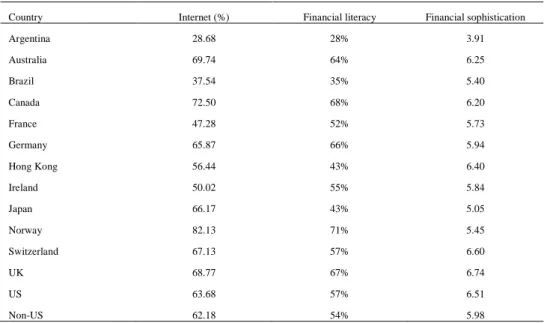
21 Some literature measure investor sophistication through different country level proxies, like the use of Internet, the financial literacy and the level of financial sophistication.
Garcia (2001) studies the information of stocks that is provided by the use of internet. Internet presents influence the bid and ask prices with size and the information of each market makers. Furthermore, each trade is presented in details with their price, volume, trade time and the percentage of each time. Through these detailed information of market, investors have a better understanding of the tendency of trade market and are better able to manage their assets.
Klapper et al. (2015) investigate the understanding of adults in financial products and decision across countries and varied from men to women. The results point out that women and the poor are lower financial literacy, but the differences are not substantial as a worldwide gap, since financial literacy is absent in the emerging market China and South Africa. Moreover, financial literacy is served as skills to manage their bank accounts and credit cards, but could not reflect the ability to get required financial services. Overall, investors with higher financial literacy manage their assets more rationally in more developed country.
Calvet (2009) constructs an index of financial sophistication in Swedish with three main financial mistakes, non-diversification, risky share inertia and the trend of selling winners and buying losers. This research finds that compared to self-employed and immigrant investors, the households with wealthier financial assets and larger family are more prone to make mistakes; that is having a higher index of financial
22 sophistication, which shows a little relevant with the education and financial experience. Overall, a larger and richer educated household is less likely to make financial mistakes than other households.
3. Sample and variables construction 3.1 Sample description
The data for this paper are drawn from the Lipper Hindsight survivor-bias free database, which collects these data from fund management companies directly. The sample consists of all open-end and actively managed equity funds during the period 1998 to 2010, but excludes off-shore funds, close-end, funds of funds and index funds. As the multiple share classes possible may lead us to count funds twice, we restrict the sample to primary fund, defined as the share class with the highest total net assets in Lipper. Ferreira et al (2012) points out that Lipper listed multiple share classes as separate funds even though these funds have the same holdings, the same manager, and the same return before expense and loads. The initial sample includes 39,564 equity funds investing both domestically and internationally.
Investment Company Institution (ICI, 2010) provides aggregate statistics of mutual funds in 31 countries, which could use to check the coverage of the database from Lipper Hindsight. At the end of 2010, ICI recorded 28,600 equity funds while Lipper reported 27,742, 97% coverage of mutual funds. Moreover, total net assets (TNA) of equity funds included all share class are recorded in Lipper and ICI, $12.8
23 and $14.5 respectively, implying that the dataset from Lipper accounts for 88% of total net assets of equity funds around the world.
In order to draw some meaningful conclusions from our analysis of different countries, we impose some restrictions on the sample. Fund size and returns use quarterly data and monthly data respectively. Mazur (2016) argue that performance persistence is considered in term of risk-adjusted return. Elton et al. (1996) points out that the sample of risk-adjusted return should be continuous while conducting the regression. Thus, the monthly observations for returns in our sample are restrict to at least 24 continuous monthly observations, which ensure that the observations are sufficient to evaluate the risk-adjusted performance. To avoid contingency of data, the country included in our sample should own at least 10 funds per quarter. Thus, we get a sample including 16,210 active open-end equity funds in 31 countries from 1998 to 2010.
Table1 shows the number of funds and TNA (Total Net Assets) across countries at the end of 2010. Table 1 has two panels. Panel A present the data for all funds by country, while Panel B displays the data for institutional funds and retail funds. We require a minimum of 7 institutional funds in each country-quarter in order to include the country in our sample .
24
Table 1. Number of funds and total net asset for all sample
Panel A: numbers of funds and total net asset (TNA) for all samples by country
Country Numbers of funds TNA($ million)
Argentina 53 400 Australia 858 149813 Austria 155 14277 Belgium 423 24565 Brazil 452 59362 Canada 1.008 318925 Denmark 195 30152 Finland 169 27156 France 975 192593 Germany 300 119641 Hong Kong 76 22151 India 212 35735 Indonesia 40 4332 Ireland 491 155682 Italy 142 32897 Japan 772 73772 Malaysia 176 9985 Netherlands 96 33475 Norway 152 41818 Poland 56 7308 Portugal 63 2337 Singapore 121 12702 South Africa 131 23277 South Korea 451 36177 Spain 269 13328 Sweden 255 112178 Switzerland 241 46726 Taiwan 228 17189 Thailand 161 6198 UK 934 450873 US 2,632 3832315 All countries 12,287 5907339
According to Panel A of Table 1, at the end of 2010, there are 12,287 funds. The US funds have the biggest scale in the mutual fund industry, representing 21.42% of the total number of funds and 70.14% of total net assets (TNA). UK, is the fourth
25 highest number of funds, comes after Canada and France with 934 funds. Indonesia is the country with the lowest number of funds, only 40, while Argentina has the lowest net assets, almost one tenth of the US TNA.
Panel B: Number of funds with institutional funds by country
Country Institutional funds Retail funds
Number Number (% of all) Number Number (% of all)
Argentina 7 13.2% 46 86.8% Australia 175 20.4% 683 79.6% Brazil 22 4.9% 430 95.1% Canada 10 1.0% 998 99.0% France 31 3.2% 944 96.8% Germany 14 4.7% 286 95.3% Hong Kong 17 22.4% 59 77.6% Ireland 85 17.3% 406 82.7% Japan 114 14.8% 658 85.2% Norway 13 8.6% 139 91.4% Switzerland 69 28.6% 172 71.4% UK 60 6.4% 874 93.6% US 806 30.6% 1,826 69.4% All countries 1,443 11.7% 10,844 88.3%
Compared with Panel A, Panel B only includes 13 countries, omitting over half countries. Panel B shows that, the US still has the highest number of institutional funds while Argentina still the lowest. 30.6% of US funds are institutional funds, higher than in any other country. Australia and Japan have the second and third highest number of institutional funds, but the institutional funds in Switzerland has the second heaviest weight of its all funds. The country with lowest institutional number of funds is Canada, only 1.0%. Overall, most countries in final sample are developed and in general, more developed country own more institutional funds.
26
3.2 Variables construction
In this paper, we focus on differences on the flow-performance relationship between retails and institutional mutual funds. Following Del Guercio and Tkac (2002) and Chevalier and Ellison, (1997) and other literature, last returns could influence fund flows, and even non-performance-related variables have impact on fund flows. Thus, for built a meaningful regression model, we gather variables that are relevant to explain flow or performance or both and testify their collinearity. We separate this part into three sections; the first one is to generate fund flows, the second part is performance measurement and the last one is the definition of the control variables.
3.2.1 Fund flows
According to Sirri and Tufano (1998) and Ferreira et al (2012) the inflows or outflows depend on last performance, which indicate that fund flows are dependent variables in our model. As pervious literature refers that the growth of new money actually is due to new external money and inflows or outflows influence the amount of TNA directly. Thus, the new money growth rate is treated as net growth of total net assets, excluding the impact on management of the underlying assets, such as dividends and capital gain or loss. As lack of information about the timing of investment decision, we assume that fund flows occur at the end of each quarter. Fund flow for fund i in country c at quarter t is calculated as:
27 𝑭𝒍𝒐𝒘𝒊,𝒄,𝒕 =𝑻𝑵𝑨𝒊,𝒄,𝒕−𝑻𝑵𝑨𝒊,𝒄,𝒕−𝟏(𝟏+𝑹𝒊,𝒄,𝒕)
𝑻𝑵𝑨𝒊,𝒄,𝒕−𝟏 (1)
Where TNAi,c,t is the total net asset value in the local currency of fund i in country c
at the end of quarter t, and Ri,c,t is fund i’s net raw return from country c in quarter t.
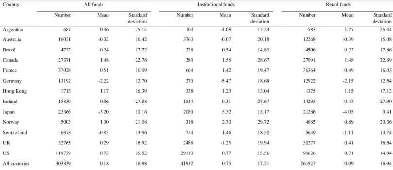
Table 2 presents summary statistics on fund flows. To prevent extreme values driving our results, fund flows are winsorized by country at the bottom and top 1% level of the distribution.
Table 2. Descriptive statistics of fund flows by country across all funds, institutional funds and retail funds
Country All funds Institutional funds Retail funds
Number Mean Standard
deviation
Number Mean Standard
deviation
Number Mean Standard
deviation Argentina 687 0.46 25.14 104 -4.08 15.29 583 1.27 26.44 Australia 16031 -0.32 16.42 3763 -0.07 20.18 12268 -0.39 15.08 Brazil 4732 0.24 17.72 226 0.54 14.80 4506 0.22 17.86 Canada 27371 1.48 22.76 280 1.56 28.67 27091 1.48 22.69 France 37028 0.51 16.09 664 1.42 19.47 36364 0.49 16.03 Germany 13192 -2.22 12.70 270 -5.47 18.68 12922 -2.15 12.54 Hong Kong 1713 1.17 16.39 338 1.23 13.04 1375 1.15 17.12 Ireland 15839 0.36 27.88 1544 -0.31 27.67 14295 0.43 27.90 Japan 23366 -3.20 10.16 2080 5.32 13.17 21286 -4.03 9.41 Norway 5003 1.00 21.08 318 2.70 29.72 4685 0.89 20.36 Switzerland 6373 -0.82 13.96 724 1.46 18.50 5649 -1.11 13.24 UK 32765 0.29 16.92 2488 -1.25 19.94 30277 0.41 16.64 US 119739 0.73 15.02 29113 0.77 15.56 90626 0.71 14.84 All countries 303839 0.18 16.98 41912 0.75 17.21 261927 0.09 16.94
28 From Table 2, Canada and Hong Kong enjoy the best average quarterly money growth rate during the sample period while Japan endures the worst growth rate. And Japan confront with two extreme situations: the institution enjoys the highest average quarterly inflows, but the retail funds has the lowest average quarterly outflows. The average institutional money growth rate among Asian countries is 3.28%, whereas the average quarterly fund flows across European is 0.08%. In general, for all countries, the average quarterly fund growth rate is above zero.
3.2.2 Performance measurement
Gruber (1996) show that raw return indicates predictive information of performance in the future, while Elton et al. (1996) argue that the risk of funds should be adjusted before measure or compared. Thus, we use raw returns and risk-adjusted returns to measure fund performance. Following Ferreira et al (2012), raw returns in our study are gross of taxes and net of total expenses included annual fees and other expenses.
Carhart (1997) employ two approaches to measure risk-adjusted performance: the Capital Asset Pricing Model (CAPM), also called Jensen’s alpha and four-factor alpha model. According to CAPM model, the return of funds in next period are predicted by the estimated beta and the excess market return. Jensen’s alpha evaluates the ability of the active manager, that is the differences between the realized return and predicted return from CAPM model.
29
𝜶𝒋,𝒊,𝒕 = 𝑹𝒊,𝒕− [𝑹𝒇,𝒕+ 𝜷𝑴,𝒊,𝒕∗ (𝑹𝑴,𝒕−𝟏− 𝑹𝒇,𝒕−𝟏)] (2)
Where Ri,t is the realized returns of fund i at the end of quarter t, Rf,t and R f,t-1are the realized return from corresponding free-risk benchmarks in quarter t and
t-1(treasury bills returns in the US), βM,i,t is the estimated beta in the industry of fund i
at quarter t, and RM,t-1 are the realized market return in quarter t-1.
Above function is the main idea to compute Jensen’s alpha, and some different details are remarkable for domestic funds and international funds. Our alphas are from Ferreira et al. (2012). They firstly compute estimated beta by regressing the previous 36 months of fund excess returns on the local market excess returns. Then they predict the return of fund in next quarter with the estimated beta and the realized excess market return. Finally, the Jensen’s alpha in next quarter are the differences between the realized return in next quarter and the predicted return.
For international funds, the computation is the same as domestic funds except that the local excess market return is replaced by region market excess return, treated market excess returns of all countries in the region the same weight of value. Ferreira et al. (2012), divide the geographic focus into four regions (Europe, Asia–Pacific, North America, Emerging Markets) based on Lipper geographic focus field. Following Carhart (1997) four-factor alpha is calculated by Fama and French’s(1993) 3-factor model plus an one-year momentum factor. In other words, the computation of four-alpha alpha for domestic funds is similar to Jensen’s alpha, except that the
30 market factor in Jensen’s alpha is replace by the market, size, value, and momentum factors.
Four-factor alpha of fund i at quarter t from four-factor model is calculated as:
𝜶𝒊,𝒕 = 𝑹𝒊,𝒕− 𝑹𝒇,𝒕− (𝜷𝑴,𝒕𝑴𝑹𝑭𝑴,𝒕−𝟏+ 𝜷𝑺𝑴𝑩,𝒊𝑺𝑴𝑩𝒕−𝟏+ 𝜷𝐇𝐌𝐋,𝐢𝑯𝑴𝑳𝒕−𝟏
+𝜷𝐌𝐎𝐌,𝐢𝑴𝑶𝑴𝒕−𝟏+ 𝝐𝟏,𝒕−𝟏) (3)
where MRFM,t-1 is the excess return of market at quarter t-1; SMBt-1 is the
difference between the monthly average return on three small portfolios and the average return on three large portfolios at quarter t-1; HMLt-1 is the average return on
two value portfolios minus the average return on two growth portfolios at quarter t-1; MOMt-1 is the average return of two 12-month high prior portfolios minus the average
return of the two low-prior portfolio in the past year.
For international funds, the computation is the combination of four-factor alpha for domestic funds and Jensen’s alpha for international funds. The market, size, value and momentum factors are calculated for each region, as value-weighted average of corresponding factor for all countries in the region.
31
Table 3 fund variables
Panel A. Fund-level variables averaged across fund quarter by country
Country Raw return(%) One-factor alpha (%)
Four-factor alpha
(%) TNA ($M) TNA family ($M) Age (year) Fee (%) SMB(%) HML(%)
Countries fund sold Argentina 5.12 -0.68 -0.47 9.73 57.78 8.02 3.48 -0.25 -0.03 1.00 Australia 0.52 0.70 0.99 167.95 5435.93 8.50 1.69 -0.10 -0.07 1.13 Brazil 3.69 2.47 2.44 131.51 3952.26 7.82 2.08 0.15 -0.18 1.00 Canada 1.19 0.20 0.15 267.58 10906.84 11.08 2.93 0.15 0.04 1.00 France 0.64 -0.71 -0.67 171.37 6131.95 11.57 2.07 0.12 -0.03 1.35 Germany 0.48 -0.94 -0.55 318.38 12367.77 13.35 2.06 0.02 -0.08 1.87 Hong Kong 2.59 0.99 1.68 177.38 3008.56 13.70 2.21 0.06 -0.18 2.80 Ireland 1.29 -0.43 -0.14 246.03 2864.92 7.58 2.34 0.05 -0.05 7.26 Japan 1.08 -0.75 -0.93 73.74 8103.31 8.43 1.89 0.10 0.01 1.00 Norway 2.71 0.85 0.87 138.27 2158.38 9.98 1.95 0.18 0.01 1.54 Switzerland 1.20 -0.10 -0.15 199.20 8798.61 13.63 2.06 0.04 -0.01 1.41 UK 1.57 -0.16 -0.16 399.60 9142.69 15.43 2.06 0.21 -0.04 2.07 US 1.74 -0.01 0.19 1267.93 51246.14 12.57 1.65 0.06 -0.04 1.05 Non-Us 1.17 -0.19 -0.13 229.05 7609.62 11.24 2.17 0.10 -0.03 1.57 All Countries 1.39 -0.12 0.00 638.46 24806.20 11.76 1.96 0.08 -0.03 1.92
32
Panel B. Pairwise correlation of fund-level variables
1 2 3 4 5 6 7 8 9 10 11 Raw return 1 One-factor alpha 0.44 1 Four-factor alpha 0.35 0.81 1 TNA 0.03 0.04 0.04 1 TNA family 0.01 0.02 0.02 0.55 1 Flows 0.07 0.07 0.05 0.10 0.02 1 Age -0.01 0.01 -0.01 0.37 0.20 -0.03 1 Fee -0.01 -0.01 -0.01 -0.14 -0.10 0.01 -0.04 1 SMB -0.01 0.03 -0.01 -0.01 -0.03 0.01 0.00 0.07 1 HML 0.02 0.01 -0.16 0.01 -0.02 0.02 0.05 0.02 0.00 1
Countries funds sold 0.01 0.01 0.01 0.11 0.09 0.02 0.07 0.03 -0.01 -0.01 1
Panel A of table 3 present fund performance statistics by country. Argentina, Brazil and Norway have the highest average raw returns, and Germany and Australia the lowest, far lower than average raw return for all countries (1.39%). Through the average Jensen’s alpha and four-factor alpha, the capacity of active managers is clearly exhibited in each country. we could see that managers in Brazil and Hong Kong perform best of the market, while managers in Germany, Japan and France have most underperformance. The average one-factor alpha is -0.12% across all countries per quarter and the average four-factor alpha equal to zero in our sample. The results reconfirmed the previous studies that in general the ability of active management of mutual fund industry could not beat the passive management around the world (Gruber, 1996; Malkiel,1995).
33
3.2.3 Control variables
Fund size determines fund flows, as flows react to last performance and larger funds capture more fund inflows (e.g., Carhart ,1997; Chevalier and Ellison,1997; and Sirri and Tufano, 1998). We use total net asset measuring fund size and include TNA as a control variable. We also use TNA family (fund family size) to explain flows, as many studies show that fund family size has a strong impact on cash flow to a member fund and larger fund size exists “star effect”, attracting more inflows, including Nanda et al. (2004), Brown (2012) and Khorana and Servaes (1999). Following Ferreira et al. (2012) we also include fund age as an explanatory variable. Karceski (2002) and Berk Green (2004) find that expenses are significant and negative with flows and performance, and hence we include fees into our model.
We also include several special factors to explain flows in our study. First, according to Carhart (1997), fund styles have an impact on fund flows. We measure the loadings on SMB and HML (the factors of Fama and French’s model) and include these loadings as additional variables of mutual funds. Finally, like Ferreira et al. (2012), we include the number of countries where the funds register to sell as an explanatory variable, as the increasing number of countries sold would influence the flows that the fund attract.
Table 3 also presents mutual fund additional variables which important in explaining flows and its sensitivity to performance. Through Panel A, the data infers that funds in more developed countries generally are older and larger with lower fees, especially the US and the UK. Argentina, the youngest market with the smallest fund
34 size and most expensive fees, is contrary to the US. Fund family size is consistent with fund size by country; that is, in general, the country with larger funds also has the larger fund family. Most country markets are overweight in small-cap funds excluding Argentina and Australia. Funds from Argentina, Brazil, Canada, Japan and the US are sold only in their domestic markets and Ireland’s funds are sold in more number of countries.
Panel B of table 3 presents the pairwise correlation matrix among fund control variables. Since the coefficients of the correlation are generally low, multicollinearity among these variables seems to be week, suggesting that these control variables can be included together in the flow-performance regressions. These pairwise correlations are all statistically significant at 5% level.
4. Methodology
In this Section, we introduce the main methodologies that we use to measure the flow-performance relationship of retail and institutional funds.
4.1 The flow-performance sensitivity
We start by using a linear model to see the links between fund flows and performance, as many studies show that the flow-performance relationship is convex (e.g. Ferreira et al., 2012; Chevalier and Ellison, 1997). We treat institutional funds as a dummy variable, which is one if the fund is institutional and zero otherwise. We then regress fund flows on last returns with control variables presented in section 3.
35 Moreover, we start by measuring the flow-performance relationship for all funds in our sample and we also measure the flow-relationship in the US and outside the US, since the number of funds in US are highest and total net assets in US accounts for more than half of TNAs in all countries.
Worldwide fund flow for fund i at the end of quarter t is calculated as:
Flowi,t=a+bi, × performance i,t-1+ci × dummy institutional fundi,t-1
+di control variablesi,t-1+𝜀𝑖,𝑡 (4)
Where a, bi,, ci,di, are the coefficients and performance i, t-1 is performance in
local currency in fund i at the end of quarter t-1. All regressions included country and time fixed effects and p-values are heteroskedasticity-robust and clustered by country. Because our aim is to measure whether the sensitivity of flow-performance for retail and institutional funds is different, in Equation 5 we add the interaction between past performance and the dummy institutional funds.
Worldwide fund flow for fund i at the end of quarter t is calculated as:
Flowi,t=a+bi, × performance i,t-1+ci × dummy institutional fundi,t-1
+ d𝑖 × performance i,t-1 × dummy institutional fundi,t-1
36
4.2 The flow-performance relationship with institutional funds
As we refer in performance measurement earlier, we measure performance using raw return, one-factor alpha and four-factor alpha. Sirri and Tufano(1998) and Ferreira, et al. (2012) show that the fund flows react differently to favorable performance and poor performance. And hence, we use a piece-wise linear model to examine the sensitivities of different flow-performance at different level performance. Like Huang et al (2007) and Ferreira, et al. (2012), we separate funds into low, medium and high three groups based on last returns. Low groups are ranked the lowest performance quintile of funds, medium group consists of three middle quintile performance-ranked funds, and high group includes funds with performance ranked in the top quintiles. To testify the asymmetric impact of institutional funds on flow-performance relationship, we interact the dummy variable institutional funds with rank performance.
The regression of interaction between institutional funds and ranked performance is computed as:
Flowi,t=a+b1 × Low i,t-1+β1 × Low i,t-1 × institutional fundi,t-1 +b2 × Mid i,t-1+β2 × Mid i,t-1 × institutional fundi,t-1
+b3 × High i,t-1+β3 × High i,t-1 × institutional fundi,t-1
+ci ×control variablesi,t-1+𝜀𝑖,𝑡 (6)
Where Low i,t-1, Mid i,t-1 and High i,t-1 are the performance of the fund i respectively ranked in the lowest quintile, three middle quintile and the highest quintile at the end of quarter t-1, and the coefficients β1, β2 𝑎𝑛𝑑 β3 represent the marginal institutional investors respond to performance.
37 For this three-piece wise model, we run the regression in the same way as in the linear model that measure the asymmetric interaction between institutional investors and also split the flow-performance relationship into the US and non-US countries. Furthermore, we also add country and time fixed effect into our regression results, like we did in the linear regression. Finally, we run a Wald test for testing the homogeneity among different level performance; that is, to test whether the difference of the slopes in low group and high group is significant.
5. Results
Our study highlights institutional funds as an important determinant of the flow-performance relationship. In this section, we present the empirical results of the regression model described in section 4. The results are displayed in Table 4 of which Panel A presents the linear model of flow-performance relationship and Panel B presents the three-piecewise model. Performance is measured using both raw returns and four-factor alpha. The results for one-factor alpha are presented in the Appendix.
38
Table 4 The impact of institutional funds on flow-performance relationship Panel A: The flow-performance measured by linear regression
Raw returns Four-factor alpha
All Countries Non-US US All Countries Non-US US
(1) (2) (3) (4) (5) (6) (7) (8) (9) (10) (11) (12)
Performance 7.08*** 7.03*** 5.646*** 5.82*** 8.0752*** 8.0833*** 5.6977*** 5.6168*** 4.1329*** 4.2397*** 6.7136*** 6.7169***
0.000 0.000 0.000 0.000 0.000 0.000 (0.00) (0.00) (0.00) (0.00) (0.00) (0.00)
Performance x Institutional fund 0.4268 -2.7947*** -0.0367 0.6375* -1.6568** -0.0153
(0.25) 0.000 (0.94) (0.06) (0.01) (0.97)
Institutional fund -0.0578 -0.2744 0.8513** 2.2897*** -0.3920*** -0.3735 -0.0114 -0.3298 0.8975** 1.7421*** -0.3505** -0.3429
(0.72) (0.28) -0.020 0.000 (0.01) (0.11) (0.94) (0.16) (0.01) (0.00) (0.01) (0.15)
Log Size -0.5993*** -0.5991*** -0.5800*** -0.5798*** -0.6156*** -0.6156*** -0.5755*** -0.5745*** -0.5615*** -0.5618*** -0.5819*** -0.5819***
0.000 0.000 0.000 0.000 0.000 0.000 (0.00) (0.00) (0.00) (0.00) (0.00) (0.00)
Log Family Size 0.2135*** 0.2136*** 0.1306*** 0.1292*** 0.2510*** 0.2510*** 0.2238*** 0.2237*** 0.1432*** 0.1429*** 0.2562*** 0.2562***
0.000 0.000 0.000 0.000 0.000 0.000 (0.00) (0.00) (0.00) (0.00) (0.00) (0.00) Log Age -0.9925*** -0.9927*** -0.8289*** -0.8295*** -0.9992*** -0.9991*** -0.9516*** -0.9531*** -0.7806*** -0.7778*** -0.9663*** -0.9662*** 0.000 0.000 0.000 0.000 0.000 0.000 (0.00) (0.00) (0.00) (0.00) (0.00) (0.00) Fee -0.0831** -0.0831** -0.088 -0.088 -0.0524* -0.0524* -0.0849** -0.0852** -0.0834 -0.0831 -0.0625** -0.0625** -0.030 -0.030 -0.140 -0.140 -0.080 -0.080 (0.03) (0.03) (0.16) (0.16) (0.04) (0.04) Flows 0.1632*** 0.1632*** 0.1067*** 0.1065*** 0.2905*** 0.2905*** 0.1699*** 0.1699*** 0.1110*** 0.1109*** 0.3025*** 0.3025*** 0.000 0.000 0.000 0.000 0.000 0.000 (0.00) (0.00) (0.00) (0.00) (0.00) (0.00) SMB -0.2014 -0.2015 -0.2118 -0.2193 -0.4207** -0.4205** -0.0366 -0.0334 -0.1329 -0.1376 0.1156 0.1157 (0.38) (0.38) (0.31) (0.29) (0.04) (0.04) (0.88) (0.89) (0.54) (0.52) (0.57) (0.57) HML 0.2873 0.2876 0.1608 0.1475 0.1266 0.1267 1.5585*** 1.5561*** 1.0814*** 1.0830*** 1.7164*** 1.7165*** (0.17) (0.17) (0.38) (0.42) (0.35) (0.35) (0.00) (0.00) (0.00) (0.00) (0.00) (0.00)
Country fixed effects Yes Yes Yes Yes Yes Yes Yes Yes Yes Yes Yes Yes
Time fixed effects Yes Yes Yes Yes Yes Yes Yes Yes Yes Yes Yes Yes
Adjusted R-squared 0.062 0.062 0.037 0.037 0.151 0.151 0.057 0.057 0.033 0.033 0.144 0.144
Number of observations 303839 303839 184100 184100 119739 119739 303839 303839 184100 184100 119739 119739
39 In panel A of table 4, the results of four-factor alpha confirm the results from raw returns. Through the statistics from panel A, one considerable important result is that the interaction between institutional fund and performance in the US differs from outside the US. In Column (4) and (10), the coefficients of non-US countries are negative and significant, meaning that the institutional investors react less to the past performance than the retailer investors do. Whereas, in Column (6) and (12), the coefficients are positive but insignificant for the US. It looks like in the US there are no differences between institutional and retail investors, implying that they both react the same way or have the same degree of sophistication. Overall, institutional investors seems to be significantly more sophisticated than retail investors when we put all countries together (in Column (8)).
Another remarkable result is that there is a significant difference in the level of flows obtained by institutional funds both in the US and Outside the US. In Column (3) and (9), the coefficients of institutional fund are positive and significant, meaning that in non-US countries institutional funds get more flows, while in Column (5) and (11) are negative and significant, meaning that in the US institutional funds get less flows (retail funds get more). This may be explained with non-US countries investors being less sophisticated and therefore there are less investors (non-institutional) investing in mutual funds. In the US is the opposite. More sophisticated market and so there are more non-institutional investors investing.
The coefficients on the remaining control variables show that little difference between the US and non-US. Most control variables are significant positive related to
40 flows except transaction costs. Investors from all countries are attracted by the herding effect that they are fond of larger funds or a member of larger fund family, older funds and the funds with more inflows. But they avoid high costly funds, as Huang et al (2007) and other literature show that higher fees increase the baseline of returns. Comparing to growth funds, investors from all countries prefer value funds.
41
Panel B: The flow-performance measured using three pieces model
Raw returns Four-factor alpha
All Countries Non-US US All Countries Non-US US
(1) (2) (3) (4)) (5)) (6)) (7) (8) (9) (10) (11) (12)
Low t-1 7.5755*** 7.2538*** 7.8408*** 7.9524*** 6.5523*** 5.3078*** 8.2163*** 7.4670*** 7.7174*** 6.4717*** 7.6252*** 7.4764***
(0.00) (0.00) (0.00) (0.00) (0.00) (0.00) (0.00) (0.00) (0.00) (0.00) (0.00) (0.00)
Low x institutional fund 3.5148 -2.7085 6.5766** 7.1974*** 19.6364*** 1.0209
(0.16) (0.60) (0.02) (0.01) (0.00) (0.72)
Mid t-1 5.6782*** 5.5615*** 4.2140*** 4.2257*** 6.9995*** 7.2645*** 4.4797*** 4.3615*** 2.9901*** 3.2162*** 5.7128*** 5.5398***
(0.00) (0.00) (0.00) (0.00) (0.00) (0.00) (0.00) (0.00) (0.00) (0.00) (0.00) (0.00)
Mid x institutional fund 0.7597 -0.0641 -1.1414* 0.8008 -3.1098*** 0.7307
(0.20) (0.95) (0.06) (0.15) (0.00) (0.25)
High t-1 17.5386*** 18.0502*** 14.4321*** 15.9212*** 18.3913*** 17.5554*** 12.7684*** 13.4809*** 9.4939*** 10.0178*** 13.7504*** 14.8558***
(0.00) (0.00) (0.00) (0.00) (0.00) (0.00) (0.00) (0.00) (0.00) (0.00) (0.00) (0.00)
High x institutional fund -3.7532 -24.0437*** 3.9576 -5.6495* -8.7917* -5.6368
(0.20) (0.00) (0.32) (0.07) (0.09) (0.16)
Institutional fund -0.0207 -0.8308* 0.8734** 1.8397** -0.3412** -1.2732*** 0.0082 -1.4559*** 0.9056** -1.5889* -0.3211** -0.6312
(0.90) (0.05) (0.02) (0.04) (0.02) (0.00) (0.96) (0.00) (0.01) (0.06) (0.02) (0.20)
Log Size -0.5971*** -0.5964*** -0.5810*** -0.5805*** -0.6085*** -0.6079*** -0.5727*** -0.5712*** -0.5629*** -0.5615*** -0.5736*** -0.5730***
(0.00) (0.00) (0.00) (0.00) (0.00) (0.00) (0.00) (0.00) (0.00) (0.00) (0.00) (0.00)
Log Family Size 0.2143*** 0.2144*** 0.1301*** 0.1281*** 0.2528*** 0.2532*** 0.2232*** 0.2234*** 0.1439*** 0.1429*** 0.2530*** 0.2532***
(0.00) (0.00) (0.00) (0.00) (0.00) (0.00) (0.00) (0.00) (0.00) (0.00) (0.00) (0.00) Log Age -0.9848*** -0.9839*** -0.8245*** -0.8195*** -0.9941*** -0.9941*** -0.9451*** -0.9456*** -0.7790*** -0.7734*** -0.9587*** -0.9571*** (0.00) (0.00) (0.00) (0.00) (0.00) (0.00) (0.00) (0.00) (0.00) (0.00) (0.00) (0.00) Fee -0.0832** -0.0832** -0.0881 -0.0880 -0.0493* -0.0488 -0.0838** -0.0840** -0.0823 -0.0820 -0.0607** -0.0607** (0.03) (0.03) (0.14) (0.14) (0.10) (0.10) (0.03) (0.03) (0.17) (0.17) (0.04) (0.04) Flows 0.1619*** 0.1618*** 0.1060*** 0.1057*** 0.2877*** 0.2877*** 0.1693*** 0.1692*** 0.1107*** 0.1105*** 0.3013*** 0.3012*** (0.00) (0.00) (0.00) (0.00) (0.00) (0.00) (0.00) (0.00) (0.00) (0.00) (0.00) (0.00)
Country fixed effects Yes Yes Yes Yes Yes Yes Yes Yes Yes Yes Yes Yes
Time fixed effects Yes Yes Yes Yes Yes Yes Yes Yes Yes Yes Yes Yes
Adjusted R-squared 0.063 0.063 0.037 0.037 0.152 0.152 0.058 0.058 0.033 0.033 0.145 0.145
Number of observations 303839 303839 184100 184100 119739 119739 303839 303839 184100 184100 119739 119739 Wald test βHigh=βLow
(p-value) 0.0000 0.0007 0.0000 0.0113 0.3146 0.0007
42 Regarding Panel B, the results on Columns (1), (3), (5), (7), (9), and (11), we can see that the flow–performance relationship is convex, as investors buy significantly more top performers than they sell funds that perform poorly. The difference between the coefficient on last year top and bottom performers (High-Low) is statistically significant as confirmed by the Wald test presented at the bottom of Table 4, Panel B. According to the literature, see, e.g. (Ferreira, Keswani, Miguel, and Ramos, 2012), more sophisticated investors sell poor performance funds, and buy more top performance funds
The figure of Panel B confirms the results in Table 4, Panel A, that institutional investors in the US interact differently from those outside US. In non-US countries, institutional investors react more to poorly performance funds, although the results are only significant when performance is measured using four-factor alpha, and less to top performers. For the US, the results are not statistically significant for both bottom and top performers, confirming that there are not differences in the level of sophistication between US retail and institutional investors.
The flow-performance relationship for institutional funds outside the US is less convex, when comparing with retail investors. Therefore, these funds contribute to decrease the overall flow-performance convexity in these countries.
43
6. Explaining the flow-performance relationship across countries
In Section 5, we present the differences of flow-performance relationship while pooling funds in all countries, US and non-US country. We expect the variation of investor sophistication across countries to explain the differences of flow-performance relationship. Ferreira et al (2012) defined sophistication as “not chasing winners but selling losers as performance persists for poor performers but not for top performers”. Accordingly, we hypothesize that more investor sophistication attribute to less convexity.
To confirm our hypothesis, we use proxies to measure investor sophistication. Internet are considered as a sophisticated channel to access information or spread characteristics of funds with less costs and convenience, and “smart” investors use Internet to achieve their investment goals, especially middle class; and hence we serve the percentage of population using the Internet as one proxy (Garcia, 2001; Findings ,2013; Ferreira et al., 2012). We expect the proportion of investors using the internet increasing with development mutual fund industry.
We also include financial literacy as investor sophistication proxy. Financial literacy is defined as the percentage of adults with financial education and understanding of various financial areas. In other words, financial literate has the ability of making appropriate decision on personal finance like investing, borrowing and so on, and financial literacy is the proportion of financial literate accounts for adults. Lusardi (2007) and Rooij et al. (2011) show that the household with low financial literacy are less likely to make wise investment management indicating that