Automatic Systems Diagnosis
Without Behavioral Models
Shekhar GuptaPalo Alto Research Center USA
Rui Abreu
Department of Informatics Engineering University of Porto, Portugal
Johan de Kleer Palo Alto Research Center
USA Arjan J.C. van Gemund
Department of Software Technology Delft University of Technology, The Netherlands
Abstract— Recent feedback obtained while applying Model-based diagnosis (MBD) in industry suggests that the costs in-volved in behavioral modeling (both expertise and labor) can outweigh the benefits of MBD as a high-performance diagnosis approach. In this paper, we propose an automatic approach, called ANTARES, that completely avoids behavioral modeling. Decreasing modeling sacrifices diagnostic accuracy, as the size of the ambiguity group (i.e., components which cannot be dis-criminated because of the lack of information) increases, which in turn increases misdiagnosis penalty. ANTARESfurther breaks the ambiguity group size by considering the component’s false negative rate (FNR), which is estimated using an analytical ex-pression. Furthermore, we study the performance of ANTARES for a number of logic circuits taken from the 74XXX/ISCAS benchmark suite. Our results clearly indicate that sacrificing modeling information degrades the diagnosis quality. However, considering FNR information improves the quality, attaining the diagnostic performance of an MBD approach.
T
ABLE OFC
ONTENTS 1 INTRODUCTION. . . 1 2 SFL . . . 2 3 ANTARES . . . 3 4 EXPERIMENTALRESULTS. . . 5 5 CONCLUSION . . . 6 REFERENCES . . . 6 BIOGRAPHY . . . 71. I
NTRODUCTIONIn model-based diagnosis (MBD) the cost of the diagnostic process can be broken down into modeling and solution cost. Solution cost includes algorithmic as well as identification penalty (pointlessly testing any incorrectly diagnosed candi-dates), where identification cost is often used as diagnostic utility measure. Traditionally, MBD studies the trade-offs be-tween the above cost dimensions in a model-once-diagnose-often context, where modeling cost is amortized over many observations.
While solution cost has been an important success factor (especially in time-critical applications), a recent design and maintenance case study in Dutch industry suggests that mod-eling cost is much more of a bottleneck for the acceptance of MBD than previously considered. At ASML a LYDIA -based diagnoser has successfully been used to diagnose faults in an important electro-mechanical subsystem that frequently suffered from failures [1]. It was shown that MBD can reduce solution cost from days to minutes for a once-only investment 978-1-4799-1622-1/14/$31.00 c 2014 IEEE.
of 25 man-days of modeling effort (approximately 2,000 lines of code (LOC), comprising sensor modeling, electrical circuits, and some simple mechanisms). Despite the obvious financial gains, management discontinued the project once it became clear that only 80% of the model could be obtained automaticallyfrom the system’s source code [2], [3]. In view of the continuous evolution of a large fraction of the subsystems (component upgrading, new lithographic tech-nology, many machine versions) their reluctance to embrace non-automated modeling for anything else than their core business (lithography) seems understandable. Behavioral modeling is primarily a complex, manual process which can be extremely time-intensive and error-prone. For certain systems, it is even impossible to build behavioral models. For simple components, as found in combinatorial logic circuits, a library approach to behavioral component modeling can amortize much of that cost, reducing the modeling process to compiling the structural information of the circuit into a system model. Still, there remains a considerable manual factor as components evolve and compositionality in complex systems is typically limited.
The fact that real-world software of realistic size still can-not be modeled for the purpose of efficient, automatic de-bugging [4] has led the software engineering community to investigate approaches that are not based on behavioral modeling, such as spectrum-based fault localization (SFL). Unlike MBD, in SFL the dynamic program execution profiles of tests (called spectra, hence the name SFL) is correlated with the test outcomes (pass/fail), typically by using sta-tistical similarity coefficients. The components are sub-sequently ranked in order of the likelihood that they are responsible for test failures. As the spectra are captured by automatic profiling, and as the test oracles are readily implemented from existing specifications, no modeling effort is required. Benchmark studies, as well as case studies by the authors diagnosing embedded software (100 KLOC) from Philips Semiconductors (now NXP) have shown promising results [5], [6], [7]. Recently, a model-based approach to SFL has been presented [8] where the statistical approach has been replaced by a reasoning approach. Grounded in (Bayesian) probability theory, the reasoning approach outperforms the statistical approach, in particular for multiple-faults, at poly-nomial cost due to a number of approximations within the diagnosis algorithm. In particular, as the reasoning approach is based on a generic component model no software modeling effort is involved.
In industrial situations where software and hardware is con-stantly evolving, a critical success factor in the mainstream adoption of MBD is whether modeling can be fully au-tomated. Given the results of (model-based) SFL in the software domain, in this paper, we study to what extent
(model-based) SFL can offer an alternative to MBD in the logic hardware domain. Apart from the above industrial motivation, there are two additional reasons: (1) the motiva-tion to study the relamotiva-tionship between SFL and MBD, where SFL’s greater ability to handle large time series of obser-vation data can partly compensate for its inherently limited precision compared to MBD, as well as (2) the benefits of a unified approach to simultaneously diagnosing software and hardware, particularly of interest in the embedded systems domain (e.g., abundant in the aerospace industry), where the root cause of software level failures can now be traced down to the hardware level.
This paper makes the following contributions:
(1) We present a spectrum-based diagnosis approach to logic circuits, which is part of ANTARES(AutoMAtic systems Di-agnosis wIthout behaviOral modelS ), to generate diagnosers based on circuit topology without modeling the behavior of the circuit’s components.
(2) We describe a particular ANTARES feature that auto-matically estimates the error propagation characteristics of a circuit, a critical parameter that significantly improves the quality of SFL’s Bayesian posterior probability computation. (3) We compare the performance of ANTARES with a state-of-the-art MBD approach (GDE [9]) using the 74XXX/ISCAS85 benchmark suite of logic circuits.
Our results show that for the logic circuits we studied ANTARESis indeed capable of approaching the performance of MBD, provided accurate information for each component is available on the average pass rate of tests (false negative rate, FNR) that cover the component when faulted.
Approaches that abstract specific component behavior, also known as structural diagnosis, have been proposed in the past, e.g., [10], [11], [12]. None of these approaches are able to deal with intermittent faults. The Analytic Redundancy Relation (ARR) based approach [13] is close to our approach. However, (i) it does not scale well for multiple faults, (ii) it is not studied for probabilistic framework, and (iii) it is also incapable of diagnosing intermittent fault. To the best of our knowledge, we are the first to propose the use of SFL in the multiple-fault diagnosis of logic circuits comprising both persistent and intermittent logic. Note that the technique pre-sented in this paper is orthogonal to techniques for automatic testing (the approach in this paper is started once something is found to be failing in order to pinpoint the root cause of the observed failure), such as automatic testing pattern generation [?], [?].
The paper is organized as follows. In Section 2 we briefly describe the principles behind SFL, as well as the diagnostic utility metric (identification cost) that we use to compare di-agnostic performance. In Section 3 we present the ANTARES approach to modeling hardware, featuring an analytic FNR estimation technique. In Section 4 we compare ANTARES with GDE using the 74XXX/ISCAS85 benchmark circuits. In Section 5 we summarize our contributions.
2. SFL
This section briefly reviews SFL. More detailed descriptions can be found in [8], [14]. In SFL the following is given:
• A finite set C = {c1, . . . , cj, . . . , cM} of M components of
which Mfare faulted.
• A finite set T = {t1, . . . , ti, . . . , tN} of N tests with binary
outcomes O = (o1, . . . , oi, . . . , oN), where oi = 1 if test ti
failed, and oi = 0 otherwise.
• A N × M (test) coverage matrix, A = [aij], where aij = 1
if test tiinvolves component cj, and 0 otherwise. Each row
is also called a spectrum.
For a Bayesian approach to SFL, the following additional information is also required:
• The prior fault probability of a component cj, denoted pj. • The false negative rate (FNR) of a component, denoted gj, which expresses the probability that a test involving a
component cj, when faulted, will still pass. In software
FNR is related to coincidental correctness [15] and failure exposing potential[16], while in hardware FNR is related to failure intermittency[17].
The result of SFL is a component ranking R =< cr(1), . . . , cr(j), . . . , cr(M )>, ordered in terms of decreasing
likelihood Pr(cj) that cj is at fault. In statistical approaches
to SFL Pr(cj) is approximated using statistical similarity
coefficients [18]. In this paper we will consider a reasoning approach where the Pr(cj) are posteriors based on Bayesian
probability theory.
The diagnostic utility of R is measured in terms of the identification cost Cd, which models the verification effort of
a diagnostician, going down the suspect ranking R search-ing for the actual faults (true positives). In particular, we measure the identification effort wasted on false positives (i.e., excluding the components found to be faulted). Let crdenote the actually faulted component that has the lowest
posterior in R, where r ∈ {1, . . . , M } denotes its rank in R. Then Cd = r − Mf. In our studies we will typically
consider a normalized value Cd/(M − Mf) which ranges
from 0 to 1, in order to compare across varying system sizes. Note that M − Mf is the number of actually non-faulted
components. This normalized metric is essentially the inverse of the DXC utility metric [19] for diagnosers that produce no false negatives (R includes all components so it cannot miss any faulted component).
Candidate Generation
In ANTARESR is derived from the multiple-fault diagnosis D =< d1, . . . , dk, . . . , d|D| > which is an ordered set of
all |D| minimal candidates, ordered by decreasing posterior probability Pr(dk). Each candidate dk comprises a minimal
set of components cj that, when faulted, are consistent with
all test observations (i.e., a minimal diagnosis).
Candidate generation is based on modeling each component by the generic, weak (i.e., faulty behavior is not specified) model2given by
hj =⇒ (inputs-okj =⇒ output-okj)
where hj denotes component health (true when nominal,
false when faulted), while inputs-ok and output-ok denote whether the component’s inputs and output are error-free (an error being produced by some faulted component upstream). Depending on the test outcome, each row i in spectrum matrix A yields either a pass set ({cj|aij = 1, oi= 0}) or a fail set
({cj|aij = 1, oi = 1}). It can be easily seen that a fail set
is equivalent to a conflict (set). Candidate generation is based on computing the minimal hitting sets (MHS) of all fail sets.
When faulted components are covered in a test, the fact that components have non-zero FNR leads to many pass sets. While not useful for deriving candidates the pass sets do influence a candidate’s posterior probability, and are also useful for speeding up (focusing) the MHS computation. Probability Computation
Given the typically large number of candidates in D that have equal fault cardinality, for large systems the ranking induced by the posterior probability computation is critical to diagnostic accuracy. For each observation obsi = (Ai∗, oi)
the posteriors are updated according to Bayes’ rule Pr(dk|obsi) =
Pr(obsi|dk)
Pr(obsi)
· Pr(dk|obsi−1) (1)
where Pr(dk|obs0) is computed from the priors according to
Pr(dk|obs0) = Y {j|¬hj} pj· Y {j|hj} (1 − pj)
assuming components fail independently. The denominator Pr(obsi) is a normalizing term that is identical for all dkand
need not be computed directly. Pr(obsi|dk) is defined as
Pr(obsi|dk) = Y J gj if oi= 0; 1 −Y J gj if oi= 1. (2)
where J = {j | cj ∈ dk, aij = 1} is the set of
com-ponent indices in dk covered by the test. Eq. (2) assumes
an OR-model, i.e., the test may fail if either of the faulted components fail. In general, the OR-model is an acceptable approximation [20], [8], not in the least since D’s probability mass is often dominated by single faults, even when the system has multiple faults.
R is derived from D by aggregating the posteriors of each dk
into posterior component probabilities according to Pr(cr) ≈
X
dk∈D,cr∈dk
Pr(dk)
The approximation is due to the fact that formally D should be expanded with all non-minimal candidates for the above equation to be correct. The reason for our approximation is discussed in the next section.
Implementation Details
In ANTARESwe use the STACCATOMHS algorithm [8], [21] for computing D from (A, O). STACCATOexploits pass sets in its any-time computation of the most probable minimal candidates dk. Typically, the first few hundred candidates
practically cover all posterior probability mass, after which the MHS algorithm is terminated. As a result, for random problems comprising N = 1, 000 tests and M = 1, 000, 000 components of which Mf = 1, 000 are faulted, the MHS is
diagnosed in less than 0.1 CPU second on a contemporary PC [8].
As discussed earlier, our performance metric Cd is
for-mally defined in terms of the full (non-minimal) diag-noses rather than the minimal diagdiag-noses D. For the large 74XXX/ISCAS85 circuits we are considering, however, the
c2
c1
1
0
1
c3
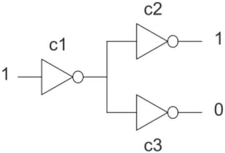
Figure 1. Three-inverter circuit
posterior probability mass covered by D is virtually equal to unity. As the number of minimal diagnoses is considerably smaller than all diagnoses, the huge computational savings outweigh the small estimation error by far. The reason for the small error is that after multiple observations are combined D already involves all components due to the use of a weak component model and the fact that the observations are random (modeling a practical application situation). Even when multiple faults are present, the latter leads to many observations that can already be explained by candidates of lower cardinality. Had we chosen to limit our observations to MFMC (Max-Fault Min-Cardinality) observations (such as generated by MIRANDA [22]) we would have to extend D with non-minimal candidates (e.g., by a low-cost, first-order extension approach such as in SEQUOIA[14]).
The posterior probability computation is a straightforward application of Bayes’ rule, implemented within the BARINEL toolset [8], using an option to externally read the gj
param-eters from file. How the gj are generated is described in
Section FNR Estimation.
3. ANTARES
ANTARES applies SFL to diagnose hardware, exploiting topological information only. Whereas in software the spectra are obtained by tracing the components that are executed per test run (dynamic control flow), in hardware a spectrum originates from a cone, i.e., all components involved in the computation of a circuit output (determined by topology). A particular feature of ANTARES is that it includes a method to estimate the gj parameters, which is vital to diagnostic
performance. In the following we outline the principle for logic circuits. Note, however, that the approach generalizes to any causal system.
Consider the example circuit shown in Fig. 1. Each primary output observation is interpreted as one test. Thus one test vector yields two tests, one which involves c1 and c2 (the
cone of the top primary output), and one involving c1and c3
(the bottom cone). Since SFL assumes the existence of test oracles, we observe a pass for the above output, and a failure for the bottom output. The observations are given in terms of A and O according to
1 1 0 +
1 0 1
-where ’+’ and ’-’ denote oi = 0 and oi = 1, respectively,
to distinguish O from A. The single conflict (c1, c3) will
0.01 (equal component types), and let gj = g = 0.5, under
the assumption that a fault will show up at the output in 50% of the cases. SFL (Eqs. 1, 2) yields the following (minimal) diagnosis D =< c3(0.67), c1(0.33) >, where Pr(dk) is in
parentheses.
The component ranking R =< c3(0.68), c1(0.37), c2(0.05) >
is computed, where Pr(cr) is in parentheses3. Note that
in this small example we have actually computed R from the full, non-minimal diagnosis, in order to include c2 in
the probability computation (since c2 is not in D). In our
74XXX/ISCAS85 experiments, however, we simply derive R from D with negligible loss of accuracy.
SFL vs. MBD
Let us compare this diagnosis with a diagnosis from MBD. Exploiting the inverter model we can now also propagate values throughout the circuit, leading to a second conflict (c2, c3). In SFL terms both conflicts are expressed as
1 0 1
-0 1 1
-which yields the minimal candidates c3, and (c1, c2).
As-suming the same priors and FNR we obtain the following diagnosis D =< c3(0.99), c1 ∧ c2(0.01) >. The derived
ranking R is < c3(0.92), c1(0.21), c2(0.21) (again, from the
full, non-minimal diagnosis). Note that the higher defect density estimation (Mf =PrPr(cr) = 1.34) compared to
the SFL solution is due to the fact that now two fail sets are found vs. one fail set and one pass set. The latter exonerates c1and c2leading to lower posteriors.
Despite the difference in posterior distribution, the diagnos-tic accuracy of both approaches are equal in terms of Cd.
However, the SFL approach suffers from the fact that no modeling information is exploited. This becomes particularly clear when considering D. While MBD correctly infers a single fault (c3 with 0.99 probability) or a double fault
(c1, c2 with 0.01 probability), SFL infers a single fault (c3
with 0.67 probability), and another single fault c1(with 0.33
probability). As the latter cannot be true SFL suffers from false positives (in terms of D) compared to MBD. However, note that typically a diagnostician will only consider R, which comprises all components anyway. Thus the diagnostic accuracy is effectively determined by the quality of the pos-terior computation, which is key in the comparison between SFL and MBD.
An aspect in favor of SFL is that it exploits the information of the pass sets, whereas MBD does not (except internally, e.g., for an MHS engine such as STACCATO, which allows better focusing, yielding computational cost reduction). This explains why c3is ranked higher than c1although, according
to SFL, both are single-fault candidates. Exploiting pass set information is one of the reasons why SFL’s diagnostic performance is of practical interest.
Ambiguity Groups
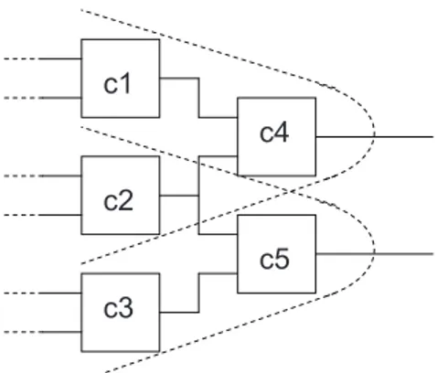
In ANTARES A directly derives from the circuit’s topology. Each of the circuit’s N0outputs generates 1 row in A, leading to N0 rows in A per test vector. For multiple test vectors A simply grows in multiples of N0 rows. Since, regardless of the number of test vectors, A only contains N0 different rows, many of the columns in A are equal. Consider the well-known systems topology in Fig. 2 which (for a single
3Note that the total probability mass (M
f) may well exceed unity.
c5
c4
c3
c2
c1
Figure 2. A well-known systems topology observation) generates the following matrix rows
1 1 0 1 0
0 1 1 0 1
Each of both cones, as well as the cone intersection, generates a set of equal columns in A. The associated components are called an ambiguity group (AG). In the above example A has three ambiguity groups (c1, c4), (c2), (c3, c5). While the
1-member AG does not pose any problem, the other 2-1-member AG’s introduce a lower bound on Cd since their member
components cannot be distinguished unless they have dif-ferent posteriors. The latter is key to our SFL approach in ANTARES.
Ambiguity Reduction
As shown by the 3-inverter example MBD generates addi-tional fail sets (conflicts) compared to SFL. Consequently, SFL gives rise to AGs that can be much larger than MBD. In software the AG problem can often be resolved by adding better tests (e.g., distinguishing components by introducing different control flow, unless they belong to the same basic block). In hardware, however, the AG problem is determined by circuit topology (which we assume static). As the ratio between the number of components and primary outputs is determined by area vs. circumference, the AG problem scales with the size of the circuit, leading to very large AGs. This implies that there are also large AGs in the ranking R (equal posteriors) if the pjand gjwould be equal, which can greatly
affect Cd. As pj is typically not available often one assumes
pj to some arbitrary value p. Even when the pj would be
different, the diagnostic performance of SFL is still largely determined by the quality of gj, as has been shown in the
software domain [23]. The reason is that gjis involved in the
Bayesian update every time a new observation is processed. In software gj is typically measured using mutation
analy-sis [24]. While these measurements significantly increase SFL accuracy, the cost of a Monte-Carlo approach scales linearly with system size. In ANTARES we therefore also consider an analytic approach to the estimation of gj since
the estimation quality is sufficient to tackle the ambiguity problem.
Gate EPP Estimation
Computing the gj of a component cj can be framed as
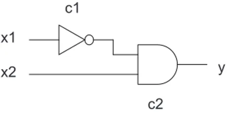
the problem of computing the error propagation probability (EPP) through a logic circuit [25], [26]. For example, con-sider the simple logic circuit according to Figure 3, compris-ing an INV gate (c1) connected to an AND gate (c2). Suppose
c2 c1
x1
x2 y
Figure 3. Example logic circuit
the INV gate is faulted. For input x = (X, 0) (X = don’t care) an error at the output of c1will be masked by the fact that c2
will always produce y = 0. However, for input x = (X, 1) an inverter error will always propagate to y. Assuming a uniform input value probability distribution, the EPP at y is 0.5, and consequently, g1= 1 − 0.5 = 0.5.
EPP in logic circuits has been studied in the context of relia-bility studies, primarily motivated by an increasing soft error rate due to ever decreasing gate sizes [25], [27]. While there exists a deterministic approach to compute the EPP through circuits of arbitrary topology given the model of each gate involved, in this paper we use a novel, probabilistic approach to EPP computation, since in the ANTARES approach we refrain from modeling the actual components. While our method produces exact estimates of the mean value of the EPP over the corresponding gate space, the EPP value found for a particular circuit output may differ from the correct value. However, a certain error is acceptable provided the posterior probability ranking by our diagnosis algorithm is not too seriously affected.
Due to space limitation, we refrain from explaining in detail how the EPP is computed. For interested readers, refer to [28]. However, in this paper, we use the general EPP model for a binary gate as derived in [28]. Let e1and e2denote that
the probability that inputs x1and x2 of the binary gate have
an error respectively. The EPP value (probability e that the gate’s output has an error) is given by
E[e] = e1+ e2− e1· e2
2 (3)
Note that Eq. (3) is averaged over the space of all 16 con-ceivable binary gate functions. Computing the EPP at circuit level simply requires composition of Eq. (3) per gate between the faulted gate(s) and the circuit output.
FNR Estimation
The above EPP model allows us to directly compute Pr(obsi|dk) for multiple-fault candidates dk in the Bayesian
update (Eq. (1)), circumventing the approach based on the single-fault gjparameters in combination with the OR-model
(Eq. (2)). However, the decreasing accuracy with increasing cardinality makes the EPP model less attractive for multiple faults. Despite the fact that the OR-model assumes failure in-dependence, its accuracy in practice outweighs the inaccuracy of a direct computation [28]. Consequently, in the following we outline an FNR estimation procedure based on the gj
parameters obtained through single-fault EPP modeling. Obtaining the EPP for single faults is straightforward. In the following we assume that a gate is either SA0 (stuck at 0) or
SA1 (stuck at 1), leading to an average failure probability of 0.5. As this gate is the only faulted gate in the circuit every subsequent gate downstream to the primary output has exactly one input that has an error. Consequently, Eq. (3) can be simplified. Without loss of generality, assume that for each gate in the path between faulted gate and primary output, x1
is in the error path. Consequently, e2= 0 and Eq. (3) reduces
to E[e] = e1/2, which implies halving the EPP per stage4.
Let mjdenote the ’depth’ of the gate cjrelative to the output
considered (for the gate at the output mj = 0). Assuming
that the faulted gate produces e = 1/2 it follows that gj is
given by
gj = 1 − 2−(mj+1) (4)
which is substituted in Eq. (2). Thus, in this model the FNR for a component is only determined by the relative topological depth of the component relative to a particular circuit output, where all (intermediate) components are modeled by the generic model of Eq. (3).
4. E
XPERIMENTALR
ESULTSIn this section we evaluate the diagnostic performance of ANTARESfor the circuits described earlier in comparison to an MBD approach. Tables 1, 2, and 3 list the diagnostic performance results for 50 random test vectors, averaged over 200 randomly injected fault sets with Mf = 1, 2, 3 faults,
respectively. Instead of Cdwe quote Cd/(M − Mf) which
allows comparison between different values of Mf (a value
of 0 indicates no identification effort, i.e., all faulted compo-nents are ranked at the top, whereas a value of 1 indicates maximum identification effort, i.e., all faulted components are at the bottom of the list).
We consider three versions of ANTARES:
• A version, denoted ABAR, where gj is not determined by
topology, but is computed internally by BARINELbased on (A, O) [8]. This reference version [29] is intended to assess the added value of using topology-specific gjinformation. • A version, denoted AMC, where gjis determined from the
circuit using Monte Carlo (MC) simulation and is externally supplied to BARINEL. This version uses the most accurate gj
information.
• A version, denoted AEPP, where gj is estimated from
the circuit using the analytical EPP model and is externally supplied to BARINEL.
In order to compare ANTARES to MBD we include results for GDE, a state-of-the-art MBD engine [9]. Since GDE does not provide posterior probabilities we have incorporated GDE within our SFL approach as follows. The additional conflicts that GDE infers due to its MBD capability are appended as rows to the A matrix obtained by ANTARES, with oi = 1.
The extended (A, O) are processed as usual using STACCATO and BARINEL.
Comparison of the ABARand MBD results shows that some diagnostic accuracy is lost by merely taking into account structure (topology) with a standard, weak component model without FNR information. The results for AMC show that knowledge of the gj has a significant impact on ANTARES’
diagnostic performance. Although the results are for logic
4As mentioned before, this differs for particular gates (1 for XOR, 1/2 for AND, etc.). Our EPP model represents the average over all 16 conceivable gates. One can improve the model once statistics are known regarding gate types.
Table 1. Cdfor ANTARESand MBD (Mf= 1)
Circuit ABAR AMC AEPP MBD 74181 0.176 0.014 0.247 0.030 74182 0.090 0.061 0.080 0.025 74L85 0.320 0.105 0.250 0.060 74283 0.096 0.034 0.155 0.050 c499 0.164 0.092 0.129 0.004 c880 0.065 0.021 0.052 0.006 c1355 0.196 0.135 0.162 0.004 c2670 0.166 0.067 0.089 0.033 c7520 0.112 0.087 0.110 0.003
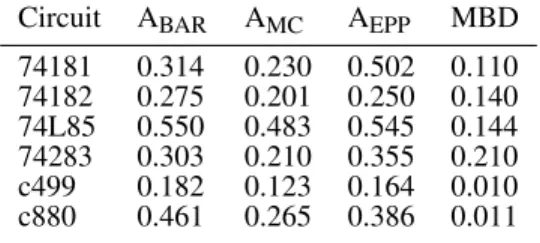
Table 2. Cdfor ANTARESand MBD (Mf= 2)
Circuit ABAR AMC AEPP MBD 74181 0.314 0.230 0.502 0.110 74182 0.275 0.201 0.250 0.140 74L85 0.550 0.483 0.545 0.144 74283 0.303 0.210 0.355 0.210 c499 0.182 0.123 0.164 0.010 c880 0.461 0.265 0.386 0.011
circuits only, these results suggest that in quite a number of cases the modeling cost associated with MBD may well outweigh the limited loss of ANTARES’s diagnostic utility. The results for AEPPshow that analytically estimating the gj
using our generic component model does not always improve ANTARES’ performance compared to not using them (ABAR). Given the impact of gj as shown by AMC, however, there is a great potential in developing more elaborate, analytic schemes. An obvious extension of the analytic EPP model takes into account information on the truth probability of a gate (in terms of its truth table). For instance, the EPP characteristics of an AND (truth probability 1/4) and an OR (truth probability 3/4) are equal to Eq. (3), while an XOR (truth probability 1/2) has higher EPP (a single error on one of its inputs always propagates to the output). In some cases the truth probability of components may be known by design, or can be measured in isolation using MC simulation. Single faults dominate the ranking yielded by random vectors since there are many single-fault diagnosis candidates that explain all failed observations. In other words, unlike MBD, our study does not make use of Max-Fault Min-Cardinality (MFMC) observation vectors, but instead use random vectors in an attempt to mimic reality. As a consequence, ANTARES suffers from a limitation in presence of multiple faults. Even for large circuits (c1355, c2670 and c7552) only one of the faulty components appears in the diagnosis and therefore ANTARES could not isolate all of them. Hence we do not include those circuit results in the paper for Mf = 2 and
3. However, in many real life scenarios, a diagnostician looking for the root cause of a system failure does not know in advance how many faults are in the system; every time a faulty component has been found and replaced, the system is typically re-tested, to ascertain that all faults have been found. With such iterative process, multiple faults often can be detected using the single fault diagnosis approach, making
Table 3. Cdfor ANTARESand MBD (Mf = 3)
Circuit ABAR AMC AEPP MBD 74181 0.480 0.460 0.608 0.287 74182 0.365 0.303 0.350 0.203 74L85 0.671 0.610 0.675 0.195 74283 0.447 0.375 0.516 0.410 c499 0.203 0.158 0.182 0.020 c880 0.502 0.321 0.452 0.020
ANTARESa useful approach.
5. C
ONCLUSIONResults clearly show that MBD outperforms every variant of ANTARES which demonstrates the importance of modeling information in diagnosis. However, there are situations where it is impossible to create behavioral models. For instance, in software of realistic size and complexity the choice not to model is typically borne out of necessity. Our industrial feedback suggests that there is a business proposition in sac-rificing some diagnostic performance in an approach where modeling is no longer required.
In this paper we addressed the trade-off between the mod-eling/identification costs in diagnosis. We also propose to exploit FNR information to boost the diagnosis quality with-out actually using the behavioral models. Our results show that ANTARES using detailed FNR information is capable of approaching the performance of MBD. While in software mutation analysis is relatively easy to implement, measuring FNR data in hardware can only be done when simulators are available. Consequently, we also studied a simple, abstract EPP modeling technique to analytically estimate the FNR data. Our results show that a more detailed EPP model is required to attain the performance of Monte Carlo measure-ments.
Future work will address improved EPP modeling to fur-ther exploit the potential of ANTARES. Currently, we use a generic component EPP model, and we will investigate whether we can reach the quality of the Monte Carlo ap-proach by dynamically measuring each component’s EPP. The great significance of such empirical study is to measure EPP without needing to inject faults in the circuit, while still not modeling component’s behavior.
A
CKNOWLEDGMENTSThis work was partially funded by FEDER/ON2 and FCT project NORTE-07-124-FEDER-000062.
R
EFERENCES[1] J. Pietersma and A. van Gemund, “Benefits and costs of model-based fault diagnosis for semiconductor man-ufacturing equipment,” in Proc. INCOSE’07, 2007. [2] B. Reeven, “Model-based diagnosis in industrial
The Netherlands.
[3] E. Schoemaker, ASML Netherlands, Personal Commu-nication, 2008.
[4] M. Nica, J. Weber, and F. Wotawa, “How to debug sequential code by means of constraint representation,” in Proc. of DX’08, September 2008.
[5] R. Mathijssen, Embedded Systems Institute, Personal Communication, 2008.
[6] P. Zoeteweij, R. Abreu, R. Golsteijn, and A. van Gemund, “Diagnosis of embedded software using pro-gram spectra,” in Proc. of ECBS’07, 2007.
[7] P. Zoeteweij, J. Pietersma, R. Abreu, A. Feldman, and A. van Gemund, “Automated fault diagnosis in embed-ded systems,” in Proc. of SSIRI’08, 2008.
[8] R. Abreu and A. van Gemund, “Diagnosing intermittent faults using maximum likelihood estimation,” Artificial Intelligence Journal, 2010.
[9] J. de Kleer, “Minimum cardinality candidate genera-tion,” in Proc. of DX’09, 2009.
[10] R. Bakker, D. van Soest, P. Hogenhuis, and N. Mars, “Fault models in structural diagnosis,” in Proc. of DX’89, 1989.
[11] A. Ducoli, G. Lamperti, E. Piantoni, and M. Zanella, “Circular pruning for lazy diagnosis of active systems,” in Proc. of DX’09, 2009.
[12] L. Gianfranco and M. Zanella, “Distributed consistency-based diagnosis without behavior,” in Proc. of DX’10, October 2010.
[13] M. Staroswiecki and G. Comtet-Varga, “Analytical redundancy relations for fault detection and isolation in algebraic dynamic systems,” Automatica, vol. 37, no. 5, pp. 687–699, May 2001. [Online]. Available: http://dx.doi.org/10.1016/S0005-1098(01)00005-X [14] A. Gonzalez-Sanchez, R. Abreu, H.-G. Gross, and
A. van Gemund, “Spectrum-based sequential diagno-sis,” in Proc. of DX’10, 2010.
[15] X. Wang, S. Cheung, W. Chan, and Z. Zhang, “Tam-ing coincidental correctness: Coverage refinement with context patterns to improve fault localization,” in Proc. of ICSE’09, 2009.
[16] G. Rothermel, R. Untch, C. Chu, and M. Harrold, “Pri-oritizing test cases for regression testing,” IEEE TSE, 2001.
[17] J. de Kleer, “Diagnosing multiple persistent and inter-mittent faults,” in Proc. of DX’07, 2007.
[18] R. Abreu, P. Zoeteweij, R. Golsteijn, and A. van Gemund, “A practical evaluation of spectrum-based fault localization,” Journal of Systems and Software, 2009.
[19] A. Feldman, T. Kurtoglu, S. Narasimhan, S. Poll, D. Garcia, J. de Kleer, L. Kuhn, and A. van Gemund, “Empirical evaluation of diagnostic algorithm perfor-mance using a generic framework,” International Jour-nal of Prognostics and Health Management, 2010. [20] L. Kuhn, B. Price, J. de Kleer, M. Do, and R. Zhou,
“Pervasive diagnosis: Integration of active diagnosis into production plans,” in Proc. AAAI’08, 2008. [21] R. Abreu and A. G. Gemund, “A low-cost
approxi-mate minimal hitting set algorithm and its application to model-based diagnosis,” in Proceedings of the 8th
Symposium on Abstraction, Reformulation, and Approx-imation, ser. SARA’09, 2009.
[22] A. Feldman, G. Provan, and A. van Gemund, “Comput-ing observation vectors for max-fault min-cardinality diagnoses,” in Proc. AAAI’08, 2008.
[23] A. Gonzalez-Sanchez, R. Abreu, H.-G. Gross, and A. van Gemund, “An empirical study on the usage of testability information to fault localization in software,” in Proc. SAC’11, 2011.
[24] J. Voas, “Pie: A dynamic failure-based technique,” IEEE TSE, 1992.
[25] H. Asadi, M. Tahoori, and C. Tirumurti, “Estimating error propagation probabilities with bounded variance,” in Proc. of DFT’07, 2007.
[26] N. Mohyuddin, E. Pakbaznia, and M. Pedram, “Prob-abilistic error propagation in logic circuits using the boolean difference calculus,” in Proc. of ICCD’08, 2008.
[27] K. Parker and E. McCluskey, “Probabilistic treatment of general combinational networks,” IEEE Trans. Comput-ers, 1975.
[28] S. Gupta, A. J. C. van Gemund, and R. Abreu, “Probabilistic error propagation modeling in logic circuits,” in Proceedings ICST’11 Workshops, ser. ICSTW ’11. Washington, DC, USA: IEEE Computer Society, 2011, pp. 617–623. [Online]. Available: http://dx.doi.org/10.1109/ICSTW.2011.40
[29] M. Wilson, “BACINOL: Bayesian circuit analysis by topology,” 2011, mSc thesis, Delft University of Tech-nology, The Netherlands.
B
IOGRAPHY[
Shekhar Gupta Shekhar Gupta is a 3rd year PhD student at Delft University of Technology (TUDelft), The Netherlands. He is on an extended research leave at Palo Alto Research Center (PARC) in Palo Alto, CA, USA. He is working in the field of Model Based Diagnosis (MBD) with Dr. Johan DeKleer. Earlier he has pursued MSc in Computer Engineering from TUDelft in 2011 with Cum Laude. He did his Master thesis with Prof. Arjan. J. C. Van Gemund on embedded system fault diagnosis. He has pursued bache-lor degree (BTech) in Information and Communication Tech-nology (ICT) from Dhirubhai Ambani Institute of Information and Communication Technology (DAIICT), Gujarat India.
Rui Abreu graduated in Systems and Computer Engineering from University of Minho, Portugal, carrying out his graduation thesis project at Siemens S.A., Portugal. Between September 2002 and February 2003, Rui followed courses of the Software Technology Mas-ter Course at University of Utrecht, the Netherlands, as an Erasmus Exchage Student. He was an intern researcher at Philips Research Labs, the Netherlands, between October 2004 and June 2005. He received his Ph.D. degree from the Delft University of Technology, the Netherlands, in November 2009, and he is currently an assistant professor at the Faculty
of Engineering of University of Porto, Portugal. He is also with the School of Computer Science of Carnegie Mellon University (CMU), USA, as a Visiting Faculty Member.
Johan de Kleer is a Principal Scien-tist in the Embedded Reasoning Area in PARC’s Intelligent Systems Laboratory. His core interest is building a system which can reason about the physical world as well as he can. Until recently, he was Laboratory Manager of PARC’s Systems and Practices Laboratory of Xe-rox’s Palo Alto Research Center. This interdisciplinary laboratory conducted research ranging from social science to robotics. Two foci of the laboratory were: (1) Smart Matter - which exploits trends in miniaturization and integration to create a new generation of products and processes that benefit from the coupling of computational and physical worlds, and (2) Knowledge - knowledge management, which includes social science research on organizations, knowledge representation and understanding images and video streams. Johan received his Ph.D. from M.I.T. in 1979 in Artificial Intelligence. He has published widely on Qualitative Physics, Model-Based Reasoning, Truth Maintenance Systems, and Knowledge Rep-resentation. He has co-authored three books: Readings in Qualitative Physics, Readings in Model-Based Diagnosis, Building Problem Solvers. In 1987 he received the pres-tigious Computers and Thought Award at the International Joint Conference on Artificial Intelligence. He is a fellow of the American Association of Artificial Intelligence and the Association of Computing Machinery.
Arjan J.C. van Gemund received a BSc in Physics, an MSc degree (cum laude) in Computer Science, and a PhD (cum laude), all from Delft University of Technology. He has held positions at the R & D organization of the Dutch multinational company DSM as an Em-bedded Systems Engineer, and at the Dutch TNO Research Organization as a High-Performance Computing Research Scientist. From 1992 he was at the Electrical Engineering, Mathematics, and Computer Science Faculty of Delft Univer-sity of Technology, the last 6 years serving as Full Professor in the area of fault diagnosis of embedded hardware and software systems. He has (co)authored over 200 scientific publications, and is (co)recipient of 8 best paper awards, and a best demo award.