Parallel Implementations of RCM Algorithm for Bandwidth
Reduction of Sparse Matrices
T.N. RODRIGUES*, M.C.S. BOERES and L. CATABRIGA
Received on November 24, 2016 / Accepted on August 5, 2017
ABSTRACT.The Reverse Cuthill-McKee (RCM) algorithm is a well-known heuristic for reordering sparse matrices. It is typically used to speed up the computation of sparse linear systems of equations. This paper describes two parallel approaches for the RCM algorithm as well as an optimized version of each one based on some proposed enhancements. The first one exploits a strategy for reducing lazy threads, while the second one makes use of a static bucket array as the main data structure and suppress some steps performed by the original algorithm. These related changes led to outstanding reordering time results and significant bandwidth reductions. The performance of two algorithms is compared with the respective implementation made available by Boost library. The OpenMP framework is used for supporting the parallelism and both versions of the algorithm are tested with large sparse and structural symmetric matrices.
Keywords:parallel RCM, bandwidth reduction, sparse matrices.
1 INTRODUCTION
Computation involving sparse matrices have been of widespread use since the 1950s, and its application includes electrical networks and power distribution, structural engineering, reactor diffusion, and, in general, solutions to partial differential equations [29]. The typical way to solve such equations is to discretize them, i.e., to approximate them by equations that involve a finite number of unknowns. The linear systems that arise from these discretizations are of the typeAx =b, in whichAis a large and sparse matrix, that is, it has very few nonzero entries. In this context, a matrix with a small bandwidth is useful in direct methods for solving sparse linear systems since it allows a simple data structure to be used. It is also useful in iterative methods because the nonzero elements will be clustered close to the diagonal, thereby enhancing data locality. Given a symmetric matrixA, a bandwidth-reduction ordering aims to find a permutation
P so that the bandwidth of P APT is small. The bandwidth of a matrix Adenoted byβ(A)is defined as the greatest distance from the first nonzero element to the diagonal, considering all
*Corresponding author: Thiago Nascimento Rodrigues – E-mail: [email protected]
rows of the matrix [29]. More formally, for thei-th row of A, i = 1,2, . . . ,n, let fi(A) =
min{j|ai j =0},andbi(A)=i− fi(A).So,β(A)= max
i=2,3,...,n{bi(A)}.
Since Papadimitrou [23] proved that the bandwidth minimization problem is NP-complete, sev-eral heuristic algorithms have been presented in the literature aiming to find good quality so-lutions as fast as possible. An important class of these algorithms treats a matrix bandwidth reduction under the perspective of a graph labeling problem. In this way, reordering a sparse matrix is considered a problem of labeling the vertices of the corresponding graph in such way that closest labels are assigned to most linked vertices.
In this paper, the parallel Unordered and Leveled implementations of the RCM algorithm pro-posed by [16] are presented. In the first one, the underlying matrix graph is completely processed in one step, followed by the permutation vector generation. On the other hand, in the second one, the graph traversing and the vector computation take place iteratively level-by-level. The original implementation of these algorithms is based on the Galois system1. However, as the OpenMP2 framework has widely been used in researches related to shared-memory parallel systems, this work analyses the results obtained by an OpenMP implementation of these algorithms. Further-more, an optimized version of each one is introduced. Actually, the set of proposed optimiza-tions leads to outstanding improvements on the performance of the algorithms. In the Unordered RCM, a strategy to reduce lazy threads is evaluated. On the other hand, the Leveled RCM is presented with an alternative main data structure – a static Bucket Array [3] – in replacement of FIFO queue [2] proposed originally. Relevant CPU time improvements were observed by means of this change.
The outline of the paper is as follow. In the next section, an overview of the serial RCM is presented. Section 3 is dedicated to description of the Unordered RCM algorithm as well as some proposed optimizations. In Section 4, the Leveled RCM algorithm is presented along with an optimized version of it. All tests and achieved results are described in Section 5. Conclusions and future works are addressed in Section 6.
2 SERIAL REVERSE CUTHILL-MCKEE
The serial Cuthill-McKee algorithm [8] is based on a Breadth-First-Search (BFS) strategy, in which the graph is traversed by level sets3. As soon as a level set is traversed, its nodes are marked and numbered. The neighbors of each of these nodes are then inspected. Each time a neighbor of a visited vertex that is not numbered is encountered, it is added to a list and labeled as the next element of the next level set. The order in which each level itself is traversed gives rise to different orderings or permutations of rows and columns. In the Cuthill-McKee ordering, the nodes adjacent to a visited node are always traversed from the lowest to the highest degree.
1Galois is a system that automatically executes serial C++ or Java code in parallel on shared-memory machines [10]. 2OpenMP is a specification for a set of compiler directives, library routines, and environment variables that can be used
to specify high-level parallelism in Fortran and C/C++ programs [22]
3A level set structure of a graph is defined recursively as the set of all unmarked neighbors of all nodes of a previous level
However, in 1971, the Reverse Cuthill-McKee algorithm was presented by [20]. It was empiri-cally observed that reversing the Cuthill-McKee ordering yields a better permutation scheme for matrix reordering problems. Algorithm 1 presents the pseudo-code of serial RCM.
Algorithm 1Serial Reverse Cuthill-McKee Algorithm
1: v1= r; // root node
2: for(i= 1t o n) {
3: Find all unlabelled neighbors of the vertexvi
4: Label the vertices found in increasing order of degree
5: }
6: Reverse the order asw1, w2, . . . , wnwherewi =vn−i+1fori =1, . . . ,n.
The rootr of the level structure is usually chosen from the pseudo-peripheral4 nodes of the associated graph. In this work, the parallel pseudo-peripheral node finding algorithm presented by [30] was implemented and used for obtaining the root vertex required by RCM.
3 UNORDERED PARALLEL REVERSE CUTHILL-MCKEE
The first RCM parallelization suggested by [16] is composed of four main steps. Based on this, the overall skeleton of the Unordered Parallel RCM is not iterative, that is, there is no a global loop wherewith the algorithm traverses the graph gradually. Instead, the four steps are executed just once and the permutation array is yielded as final output. These related steps are detailed as follow.
Step 1: Generate a level structure through the Unordered BFS algorithm. The Unordered BFS algorithm relies on the perception of local minimums in the graph regarding the levels of the adjacent nodes. More precisely, the level of every node (excepting the root) may be computed as the highest level among the respective neighbors added of one [11]. In this way, the level computation for a nodenmay be described as a fixpoint system5:
Initialization:
level(r oot)=0; level(k)= ∞, ∀kother than root; Fixed Point Iteration:
level(n)=min(level(m)+1), ∀m∈neighbors of n.
Algorithm 2 shows the pseudo-code of the implemented Unordered BFS and the respective op-timizations suggested by this work. In order to explore the fixed point feature, an unordered worklist (wl) structure must by maintained by the algorithm. A structure of this type makes pos-sible any node to be picked up. Thereafter, the algorithm is able to processing several nodes in
4A pseudo-peripheral node is one of the pairs of vertices that have approximately the greatest distance from each other in
the graph (the graph distance between two nodes is the number of edges on the shortest path between nodes).
parallel. Nevertheless, as threads access the worklist in a non-deterministic way, a node may be eventually set with a level higher than the correct final value. Despite this, the successive itera-tions executed by threads over the worklist generate a monotonic decrement of the level of each processed nodes. This decrement stabilizes at the appropriated node level (fixed point iteration).
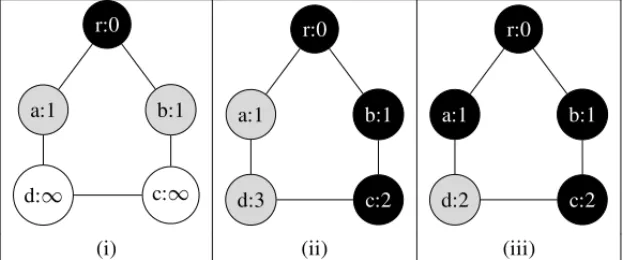
This process is exemplified by Figure 1. Initially at step (i), three nodes have already been in-spected by the algorithm. The rootr is the first node processed (black background) by a thread, and its respective neighbors are active (gray background) in the worklist. The level of them has been defined as the level of the parent (zero) added of one. At this moment, both nodes (aand
b) may be taken by a thread. Eventually, in the step (ii), the nodebwas selected and processed by a thread. Consequently, its unprocessed neighbors (just the nodec) were selected and became actives in the worklist. Next, two nodes are available to be processed:a(from the previous step) andc(from the current step). As there is no a specific order to process the nodes, anyone may be taken. In this case, the nodecwas selected and its not processed neighbor (noded) become active with the level defined as three. Finally, at step (iii), just the nodearemains in the worlist. So, it is taken by a thread, and the level of its not processed neighbor (noded) is set to the appropriated value, i.e., two.
d:∞ c:∞
a:1 b:1
r:0
d:3 c:2
a:1 b:1
r:0
d:2 c:2
a:1 b:1
r:0
(i) (ii) (iii)
Figure 1: Fixed Point Iteration Example.
Two optimizations previously presented by [11] were incorporated into the Unordered BFS (Algorithm 2).
Algorithm 2Optimized Unordered BFS Algorithm
1: Graph G = input(); // Read in graph
2: Worklist ws;
3: ws.add(root);
4: while(notws.isEmpty()) { 5: // Work Chunking
6: Worklist threadws;
7: foreach(Node n: ws) { // Atomic access to ws 8: if(threadws.size()>WORK CHUNK)break;
9: threadws.add(n);
10: }
11: // Fixed Point Iteration
12: Worklist relaxedws;
13: foreach(Node n: threadws) {
14: foreach(Node v: G.neighbors(n)) { 15: int level = n.getLevel() + 1;
16: if(level>v.getLevel()) {
17: v.setLevel(level);
18: relaxedws.add(v);
19: } } }
20: // Relaxing nodes
21: foreach(Node m: relaxedws) {
22: atomicws.add(m);
23: } } } }
2. Wasted work reduction:It was implemented a strategy to reduce the time wasted by each waiting thread (idle threads) in which all threads remove active elements from one end of the worklist and add to the other. The concurrent access of each worklist end is managed by two distinct access lock. Naturally, this approach relaxes the strict order in which the worklist is processed. However, to ensure this strict order increases the access time of the worklist beyond the benefit of reducing the amount of wasted work.
These two related optimizations were earlier explored in the work [24]. But the comparison of the parallel Unordered RCM was made against a correspondent serial algorithm implemented by [13].
to each thread that, in turn, counts how many nodes were computed by all threads in its respective range. The result is stored in the global array.
Step 3: Compute the prefix sum of levels.The prefix sum6calculus implemented in this work is based on the algorithm proposed by [1]. Initially, each thread computes the prefix sums of the
n
p elements it has locally. The total number of elements (n) corresponds to the maximum level
accounted for by the previous step of the Unordered RCM algorithm. The valuepis related to the number of threads. Hereafter, the last prefix sum of each thread is assigned to arrays responsible for guiding the data exchanging process among the threads. In fact, the local prefix sum values are exchanged and each thread accumulates the respective received value. The rule to determine a pair of threads that is going to communicate is through a XOR (exclusive OR) bitwise operation between the unique identifier of the sender thread and a constant related to the group of the receiver thread. Finally, each thread merges the result from the accumulated prefix sums with each local prefix sum initially computed.
Step 4: Build the permutation array. The underlying concept behind the operation of this phase is the pipelining of threads actions among the levels of the graph. For this, one thread is assigned for each level, and the communication among them takes place in pairs: a thread responsible for a levellplays a producer (writer) role, while a thread assigned to the levell+1 acts as a data consumer (reader). Every read/write operation happens over the permutation array. The controller of this implemented producer/consumer paradigm is done through the prefix sum array (sums) generated in the previous step. Actually, it is never changed once its values are used as bounds for threads operations. In this way, this pipeline makes possible the construction of the permutation array in a parallel way: while a thread writes the children nodes from a levellin the permutation array, another thread reads these ones in order to write the corresponding neighbors of them at levell+1 in the permutation array.
4 LEVELED PARALLEL REVERSE CUTHILL-MCKEE
The second parallelization of RCM presented by [16] makes use of a different approach. There is no an unordered execution of threads through the graph as a whole. Instead, the graph is traversed level by level, and the parallelism is restricted to one level per time. In each level-iteration, the permutation array is built gradually. The step-by-step executed by the Leveled RCM is detailed in Algorithm 3.
Iterations are composed of four steps carried out inside the outermost parallel loop (line 3). Initially, threads explore the neighbors of the parent nodes previously stored in the permutation array (lines 6-16). This expansion step sets the appropriated level of each explored neighbor. In the two next steps, the number of children (neighbors) per level is accounted (reduction step – lines 18-20), and the prefix sum is generated subsequently (lines 22-24). Finally, the neighbors processed in the current iteration are stored in the permutation array (placement step).
6The prefix sum operation takes a binary associative operator⊕, and an ordered set ofnelements[a
0,a1, . . . ,an−1]and
Algorithm 3Leveled RCM
1: Graph G = input(); // Read in graph
2: P[0] = source;
3: while(P.size<G.size)
4: // Expansion
5: Listgeneration;
6: foreach(Node parent: P[parent1:parentN]) { 7: for(Node nb: parent.neighbors) { 8: if(nb.level>parent.level) { 9: if(nb.level>parent.level + 1) {
10: // Atomic check
11: atomicnb.level = parent.level + 1;
12: generation.push(child);
13: }
14: if(parent.order<child.parent.order)
15: atomicchild.parent = parent;
16: } } } 17: // Reduction
18: foreach(Node child: generation) { 19: atomicchild.parent.chnum++;
20: }
21: // Prefix Sum
22: foreach(int threads: thread) {
23: Prefix sum of parent.chnum into parent.index
24: }
25: // Placement
26: foreach(Node child: generation) { 27: atomicindex = child.parent.index++;
28: P[index] = child;
29: if(child == child.parent.lastChild)
30: sort(P[children1:childrenM]);
31: } }
4.1 Optimized Leveled Parallel RCM
storing a node, it is used a hashing function. As this type of function may generate a same output for distinct inputs, each bucket array position is able to enqueue nodes. Figure 2 presents an operating scheme of the bucket array implemented for the optimized Leveled RCM. Furthermore, the use of the Bucket Array as main data structure produces an important impact on the design of the new proposed algorithm. In effect, the number of steps of the original algorithm were merged into just two. The algorithm idea is presented in Algorithm 4.
Figure 2: Bucket Array with hash functionh(x)=xmod 5.
Algorithm 4Optimized Leveled RCM
1: Graph G = input(); // Read in graph
2: P[0] = source;
3: while(P.size<G.size)
4: // Expansion
5: BucketArraygeneration;
6: foreach(Node parent: P[parent1:parentN]) { 7: for(Node nb: parent.neighbors) { 8: if(nb.level>parent.level) { 9: if(nb.level>parent.level + 1) {
10: // Atomic check
11: atomicnb.level = parent.level + 1;
12: if(nb.status == UNLABELED) {
13: nb.status = LABELED;
14: generation[hash(parent)].push(nb);
15: } } } } } 16: // Placement
17: foreach(Vector children: generation[bucket1:bucketN].children) { 18: atomicindex = P.size + permOffSet;
19: atomicpermOffSet += children.size;
20: sort(children);
21: foreach(Node child: children)
22: P[index++] = child;
The algorithm starts setting a pseudo-peripheral node (source node) at the first position of the permutation array. Hereafter, the parallel processing comes into play inside the outermost loop (line 3). Every iteration is composed of two steps. In the first one, all nodes to be processed are read from the permutation array (P), and the respective children of each node are inspected. A global range (parent1:parentN– line 6) is kept in order to control the parents to be processed in each iteration. Thus, the appropriated level is set to everyU N L AB E L E Dchild (line 11), the status of each one is updated toL AB E L E D(line 13), and they are stored in the correct positions in the bucket arraygenerat ion(line 14). Two features related to the use of a bucket array in this step are ever relevant for the algorithm performance:
• Implicit reduction step.As each processed child node is stored in the bucket of its respec-tive parent, the number of children per parent becomes automatically available through a simple node counter. It is incremented at each bucket insertion. Thus, there is no necessity of a separated step (reduction) for to execute this computation, as is done by the original algorithm.
• Cheap hashing function. Each cell or bucket of the main data structure corresponds to a parent node of some inspected node in the current iteration. So, the hashing function employed in mapping nodes to buckets involves just a memory address computation. In order words, to find out the correct position of a node in the bucket array is related to the cost of one memory access.
After all threads conclude the building bucket array process by means of the parent nodes inspec-tion, they advance to the second iteration step. In this phase, each thread takes a bucket and stored the children mapped to it in the final permutation array (lines 21-22). This way of traversing the processed nodes, i.e. bucket-by-bucket instead of node-by-node, represents an important im-provement for the performance of the algorithm. In effect, this strategy makes possible threads execute all placement work independently of each other. This because only two synchronized operations (lines 18 and 19) are necessary. Both of them are related to updating the range of the permutation array to be made available for the next iteration. In contrast, the original algorithm guides the threads work through the prefix sum computed in a previous step. This specific step is not necessary in the bucket-by-bucket computation proposed by the optimized algorithm.
All aforementioned modifications implemented in the original algorithm were early evaluated in a previous work [25]. However, the comparison was made against a free OpenMP-based im-plementation of the original algorithm. The evaluation shown that the Leveled RCM speedup is critically compromised by a straightforward replication of it to the OpenMP platform.
5 EXPERIMENTAL RESULTS
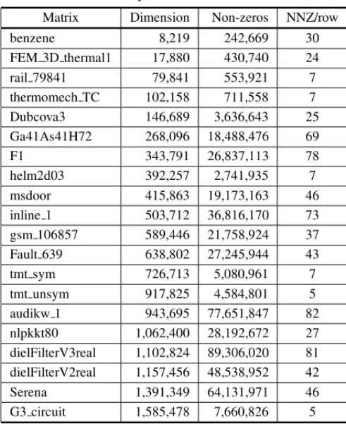
Florida Sparse Matrix Collection [9]. These matrices cover multiple type of problems in order to increase the dataset variety and the percentage of sparsity of each one is higher than 99.97%. The set of tested matrices is shown in Table 1. The columns present matrices and some characteristics of them: dimension, number of non-zeros, and average of non-zeros per row (NNZ/row). The program was coded in theC language and the parallelism was supported by OpenMP frame-work. The experiments were performed on a PC running Ubuntu Linux, version 14.04.5 LTS, with Kernel version 3.19.0-25. It consists of 2 Xeon processors of 8 cores each, operating at 2.4 GHz. Each core has a unified 256KB L2 cache and each processor has a shared 20MB L3 cache. The PC contains 32GB of main memory and code was compiled with GNU gcc version 4.8.4. The complete source code is available on GitHub repository [31].
Table 1: Sparse Tested Matrices.
Matrix Dimension Non-zeros NNZ/row
benzene 8,219 242,669 30
FEM 3D thermal1 17,880 430,740 24
rail 79841 79,841 553,921 7
thermomech TC 102,158 711,558 7
Dubcova3 146,689 3,636,643 25
Ga41As41H72 268,096 18,488,476 69
F1 343,791 26,837,113 78
helm2d03 392,257 2,741,935 7
msdoor 415,863 19,173,163 46
inline 1 503,712 36,816,170 73
gsm 106857 589,446 21,758,924 37 Fault 639 638,802 27,245,944 43
tmt sym 726,713 5,080,961 7
tmt unsym 917,825 4,584,801 5
audikw 1 943,695 77,651,847 82
nlpkkt80 1,062,400 28,192,672 27 dielFilterV3real 1,102,824 89,306,020 81 dielFilterV2real 1,157,456 48,538,952 42
Serena 1,391,349 64,131,971 46
G3 circuit 1,585,478 7,660,826 5
Tables 2 and 3 show a quality and performance comparison, respectively, among the serial Boost Library implementation of RCM and the two modified parallel versions of the algorithm, Un-ordered and Leveled, which have been proposed in this work. The algorithms were performed five times for each pair(mi,tj), wheremiis a matrix of Table 1, andtj is the number of threads
between 1 and 12 (in steps of 2) used by each algorithm. For each(mi,tj)tested pair, the
the Unordered algorithm. This same number of threadstj was used to select the corresponding
(mi,tj)tested pair from the Leveled algorithm. Moreover, the Compressed Sparse Row format
was the mechanism used to store each tested matrix. The operations applied on them were also performed using this format.
5.1 Reordering Quality
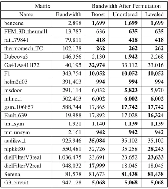
Table 2 shows the new bandwidth obtained after applying the permutation generated by each al-gorithm. In the column Bandwidth the original bandwith of the matrices is presented. The same band reordering values were reached by the three implementations for five of tested matrices. The Boost library overcomes both parallel algorithms only for three matrices: Ga41As41H72,
audikw 1, and diel Filt er V2real. For the remaining matrices, both proposed algorithms at-tained the smallest values for the bandwidth. In particular, only for theSerena matrix, the al-gorithms reached a less expressive reordering result around 0.17%. Five matrices achieved an intermediate reduction rate (up to 56.04%): Fault 639, Ga41As41H72, t mt s ym benzene, andt mt uns ym. With the other matrices, the percentage of reduction various between 95.60% (nlpkkt80) until 99.75% (helm2d03).
Table 2: Reordering Quality Comparison.
Matrix Bandwidth After Permutation Name Bandwidth Boost Unordered Leveled
benzene 2,898 1,699 1,699 1,699
FEM 3D thermal1 13,787 636 635 635
rail 79841 79,811 418 418 418
thermomech TC 102,138 262 262 262
Dubcova3 146,356 2,130 1,942 2,268
Ga41As41H72 40,195 32,974 33,112 33,016
F1 343,754 10,052 10,052 10,052
helm2d03 391,403 994 994 994
msdoor 291,114 6,032 5,823 5,970
inline 1 502,403 6,002 6,002 6,002
gsm 106857 588,744 17,865 17,742 17,742
Fault 639 19,988 17,892 17,028 16,324
tmt sym 1,921 1,140 1,139 1,139
tmt unsym 2,161 942 942 942
audikw 1 925,946 35,084 35,102 35,102
nlpkkt80 550,481 32,726 35,258 28,243
dielFilterV3real 1,036,475 23,691 23,652 23,633 dielFilterV2real 948,032 17,999 18,045 18,045
Serena 81,578 81,673 81,438 81,438
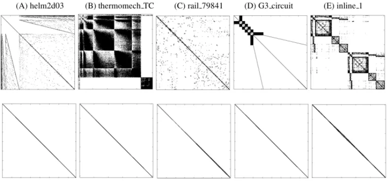
(A) helm2d03 (B) thermomech TC (C) rail 79841 (D) G3 circuit (E) inline 1
Figure 3: Sparse matrix pattern yielded by the Unordered RCM.
A strict comparison between the two proposed algorithms emphasizes the efficiency of both ap-proaches in sense of quality reordering. Both of them reached the best bandwidth value with twelve matrices. But, for two matrices (Dubcova3 andmsdoor), only the Unordered RCM at-tained the best reduction values. On the other hand, the Leveled RCM generates the best permu-tation for three other ones: Fault 639,nlpkkt80, anddiel Filt er V3real. The presented values of bandwith reduction highlight the efficiency of all approaches in sense of quality reordering.
The quality reordering may also be graphically attested through Figure 3. It shows the five ma-trices with best bandwidth reduction rate reached by the algorithms. The first row of each group presents the matrix sparsity before reordering. In the below rows, each respective matrix is exhib-ited as result of a permutation of rows and columns derived from the Unordered RCM algorithm. Actually, the reordering pattern reached by any one of the three tested algorithms might be used to depicts the quality of applied permutation. This because the differences among the bandwith reduction reached by each one is less than 0.002% and may be negligible.
5.2 Reordering Performance
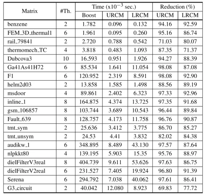
Table 3 shows the elapsed time (Time columns) by the algorithms, in scale of 10−3seconds, to
Table 3: Performance Comparison. URCM: Unordered RCM, LRCM: Leveled RCM.
Matrix #Th. Time (x10
−3sec.) Reduction (%)
Boost URCM LRCM URCM LRCM
benzene 2 1.782 0.096 0.132 94.16 92.59
FEM 3D thermal1 6 1.961 0.095 0.260 95.16 86.74
rail 79841 2 2.720 0.788 0.542 71.03 80.07
thermomech TC 4 3.818 0.483 1.093 87.35 71.37
Dubcova3 10 16.593 0.951 1.926 94.27 88.39
Ga41As41H72 6 85.534 1.641 11.054 98.08 87.08
F1 6 120.952 2.319 8.591 98.08 92.90
helm2d03 2 13.858 1.585 1.498 88.56 89.19
msdoor 4 89.861 2.402 6.323 97.33 92.96
inline 1 8 164.875 4.374 13.725 97.35 91.68 gsm 106857 8 103.744 3.689 10.543 96.44 89.84 Fault 639 8 128.757 4.173 11.758 96.76 90.87
tmt sym 2 25.636 3.412 3.775 86.70 85.27
tmt unsym 2 24.53 4.41 3.832 82.02 84.38
audikw 1 6 348.895 8.489 43.130 97.57 87.64
nlpkkt80 4 139.195 5.903 15.35 95.76 88.97
dielFilterV3real 8 404.739 9.611 53.626 97.63 86.75 dielFilterV2real 6 231.527 7.405 19.924 96.80 91.39
Serena 6 294.792 7.038 40.062 97.61 86.41
G3 circuit 2 40.042 12.080 8.923 69.83 77.72
A direct performance comparison between the two parallel approaches points out the superior efficiency of the Unordered algorithm. Indeed, the best times were reached by the Unordered RCM for sixteen tested matrices. On the other hand, the Leveled RCM obtained the best values for another subset of four instances. The time reduction percentage reached by the Unordered algorithm various between 69.83% (G3 circuit) and 98.08% (F1). Analogously, the reduction ratio obtained by the Leveled RCM was from 71.37% (t hermomech T C) to 92.96% (msdoor).
Figure 4 presents how speedups of the Unordered RCM scale as the number of threads is in-creased. Five matrices with the highest rate of speedup were selected. As shown by this figure,
Figure 4: Speedup of Smallest Matrices.
Another feature is related to the no significant speedup observed for the Leveled RCM. As it uses a different general strategy based on a parallelism by level [16], a barrier must be placed between each level. Because of this, increasing the number of threads do not necessarily lead to an improvement of performance.
6 CONCLUSIONS AND FUTURE WORKS
Both parallel implementations of the RCM presented in this work were supported by the OpenMP framework. However, some works have addressed the reordering problem through the use of an-other kind of parallelism tool. As example, [7] has developed a parallel tool for graph partition-ing, and several works have discussed the parallelization of algorithms by the Galois System [11]. Moreover, other data structures and BFS strategies have been proposed for the parallelism of RCM. In fact, Hassam et al. [11] present relevant results from a wavefront BFS implementa-tion, and Leiserson and Schardl [18] propose a novel implementation of a workset data structure, called “bag”, in place of FIFO queue usually employed in BFS algorithms. The use of these new structures and strategies might promotes more improvements to the algorithms studied in this work. Moreover, additional comparisons against other mathematical libraries may ever endorse the relevant performance reached by the algorithms. In this way, a confrontation with the Har-well Subroutine Library (HSL) [12] – a collection of state-of-the-art packages for large-scale scientific computation – constitutes an important complementary test to be made.
RESUMO. O algoritmo Reverse Cuthil-McKee (RCM) constitui uma heur´ıstica bem con-hecida para o reordenamento de matrizes esparsas. Ele ´e tipicamente aplicado para a
me-lhoria do desempenho da computac¸˜ao de sistemas lineares de equac¸˜oes. Este artigo descreve
duas abordagens paralelas propostas para o algoritmo Reverse Cuthill-McKee, assim como vers ˜oes otimizadas baseadas em alguns aprimoramentos propostos. Na primeira abordagem
h´a a explorac¸˜ao de uma estrat´egia para a reduc¸˜ao dethreadsociosas, enquanto a segunda abordagem faz uso de umbucket arrayest´atico como estrutura de dados principal, al´em de suprimir algumas etapas do algoritmo original. As modificac¸˜oes apresentadas conduzem a
re-sultados relevantes tanto em termos do tempo de reordenamento quanto na reduc¸˜ao da largura de banda. O desempenho de cada algoritmo ´e comparado com a sua respectiva implementac¸˜ao
disponibilizada pela bibliotecaBoost. O paralelismo ´e suportado peloframeworkOpenMP e ambas as vers ˜oes do algoritmo s˜ao testadas com matrizes esparsas de grande porte e estrutu-ralmente sim´etricas.
Palavras-chave:RCM paralelo, reduc¸˜ao de largura de banda, matrizes esparsas.
REFERENCES
[1] S. Aluru. Teaching parallel computing through parallel prefix, The International Conference for High Performance Computing, Networking, Storage and Analysis, (2012), Salt Lake City, USA.
[2] G. Anderson and D. Ferro & R. Hilton. Connecting with Computer Science – Second Edition. Course Technology, Cengage Learning, Boston, (2011).
[3] M.J. Atallah & S. Fox. Algorithms and Theory of Computation Handbook. CRC Press, Inc., Boca Raton, FL, USA, (1978).
[5] L. Cardelli & X. Leroy. Abstract Types and The Dot Notation, Research report 56, Digital Equipment Corporation, Systems Research Center, March 10, (1990).
[6] D. Chazan & W. Miranker. Chaotic Relaxation.Linear Algebra and its Applications,2(2) (1969), 199–222.
[7] C. Chevalier & F. Pellegrini. PT-Scotch: A Tool for Efficient Parallel Graph Ordering.Parallel Com-put.,34(6-8) (2008), 318–331.
[8] E. Cuthill & J. McKee. Reducing the Bandwidth of Sparse Symmetric Matrices, at “Proceedings of the 24th ACM National Conference”, pp. 157–172, ACM ’69, (1969).
[9] T.A. Davis & Y. Hu. The University of Florida Sparse Matrix Collection.ACM Trans. Math. Softw., 38(1) (2011), 1:1–1:25.
[10] M. Kulkarni, K. Pingali & B. Walter et al. Optimistic parallelism requires abstractions, at “Proceed-ings of the 28th ACM SIGPLAN Conference on Programming Language Design and Implementa-tion”, pp. 211–222, PLDI ’07, (2007).
[11] M.A. Hassaan, M. Burtscher & K. Pingali. Ordered vs. Unordered: A Comparison of Parallelism and Work-efficiency in Irregular Algorithms, at “Proceedings of the 16th ACM Symposium on Principles and Practice of Parallel Programming”, pp. 3–12, PPoPP ’11, (2011).
[12] Harwell Subroutine Library. A collection of Fortran codes for large scale scientific computation, (2011),http://www.hsl.rl.ac.uk/.
[13] B. Lugon & L. Catabriga. Algoritmos de reordenamento de matrizes esparsas aplicados a precondi-cionadores ILU(p), at “Simp´osio Brasileiro de Pesquisa Operacional”, pp. 2343–2354, XLV SBPO, (2013).
[14] A. George. Nested Dissection of a Regular Finite Element Mesh.SIAM Journal on Numerical Anal-ysis,10(2) (1973), 345–363.
[15] A. George & J.W.H. Liu. A Fast Implementation of the Minimum Degree Algorithm Using Quotient Graphs.ACM Trans. Math. Softw.,6(3) (1980), 337–358.
[16] K.I. Karantasis, A. Lenharth, D. Nguyen, M. Garzar´an & K. Pingali. Parallelization of Reordering Algorithms for Bandwidth and Wavefront Reduction, at “Proceedings of the International Conference for High Performance Computing, Networking, Storage and Analysis”, pp. 921–932, SC ’14, (2014).
[17] G. Karypis & V. Kumar. A Parallel Algorithm for Multilevel Graph Partitioning and Sparse Matrix Ordering.J. Parallel Distrib. Comput.,48(1) (1998), 71–95.
[18] C.E. Leiserson & T. B. Schardl. A Work-efficient Parallel Breadth-first Search Algorithm (or How to Cope with the Nondeterminism of Reducers), at “Proceedings of the Twenty-second Annual ACM Symposium on Parallelism in Algorithms and Architectures”, pp. 303–314, ACM, (2010).
[19] W. Lin. Improving Parallel Ordering of Sparse Matrices Using Genetic Algorithms. Appl. Intell., 23(3) (2005), 257–265.
[20] W. Liu & A.H. Sherman. Comparative Analysis of the McKee and the Reverse Cuthill-McKee Ordering Algorithms for Sparse Matrices.SIAM Journal on Numerical Analysis,13(2) (1976), 198–213.
in (Computer) Systems: First International ICST Conference – Proceedings”, pp. 217–228, ICST, (2011).
[22] L. Dagum & R. Menon. OpenMP: An industry-standard API for shared-memory programming.IEEE Comput. Sci. Eng.,5(1) (1998), 46–55.
[23] C.H. Papadimitriou. The NP-Completeness of the bandwidth minimization problem.Computing, 16(3) (1976), 263–270.
[24] T.N. Rodrigues, M.C.S. Boeres & L. Catabriga. An Implementation of the Unordered Parallel RCM for Bandwidth Reduction of Large Sparse Matrices, at “Congresso Nascional de Matem´atica Aplicada e Computacional”, XXXVI CNMAC, (2016), (in press).
[25] T.N. Rodrigues, M.C.S. Boeres & L. Catabriga. An Optimized Leveled Parallel RCM for Bandwidth Reduction of Sparse Symmetric Matrices, at “Simp´osio Brasileiro de Pesquisa Operacional”, XLVIII SBPO, (2016), (in press).
[26] B.S.W. Schr¨oder. Algorithms for the Fixed Point Property.Theoretical Computer Sciense,217(2) (1999), 301–358.
[27] S.W. Sloan. An algorithm for profile and wavefront reduction of sparse matrices.International Jour-nal for Numerical Methods in Engineering,23(2) (1986), 239–251.
[28] J.G Siek, L.-Q. Lee & A. Lumsdaine. The Boost Graph Library: User Guide and Reference Manual, Addison-Wesley Longman Publishing, Boston, MA, USA (2002).
[29] Y. Saad. Iterative methods for sparse linear systems, Addison-Wesley Society for Industrial and Applied Mathematics, Philadelphia, PA, USA (2003).
[30] G.K. Kumfert.An object-oriented algorithmic laboratory for ordering sparse matrices, Lawrence Livermore National Laboratory and United States, (2000).
[31] T.N. Rodrigues. tnas/reordering-library: Trends in Applied and Computational Mathematics,doi: