Article
Bootstrap estimation of resource selection probability functions
Sandra V. Cardozo1, Bryan F. J. Manly2, Raydonal Ospina3, Carlos T. S. Dias4
1
Statistics Department, National University of Colombia, Bogotá, Colombia
2
Western EcoSystems Technology Inc. Cheyenne, Wyoming, USA
3
Statistics Department, Federal University of Pernambuco, Recife/PE, Brazil
4
Statistics Department, ESALQ, University of São Paulo, Piracicaba/SP, Brazil E-mail: [email protected]
Received 6 September 2013; Accepted 10 October 2013; Published online 1 December 2013
Abstract
Resource selection functions (RSFs) are used for quantify how animals are selective in the use of the habitat
period or food. A Resource Selection Probability Function (RSPF) can be estimated if N, the total number of
units in the population, and n1 the total number of used units in the study period are both known and small. An
approximation of the RSPF can then be estimated using any standard program for logistic regression but the
variances of the estimates of the parameters are too small. Three methods of bootstrap sampling, parametric, nonparametric and a modified parametric method are proposed for the estimation of variances, with a
discussion about the limitations of logistic regression for estimating RSPF. The method for estimating the RSPF described here has potential applications in medicine, ecology and other areas.
Keywords resource selection functions (RSFs); resource selection probability function (RSPF); bootstrap; logistic regression.
1 Introduction
Using our approach the RSPF can be estimated using any standard logistic regression program but the
variances of parameter estimates that are output by the program will be too small and goodness of fit statistics will not be correct. Also, there is some small sample bias in parameter estimates. To overcome these problems bootstrap resampling of the data is proposed. Three methods for doing this resampling are described and a
simulation study indicates that one of these methods gives very satisfactory results.
The paper concludes with a discussion about some of the potential limitations with using logistic
regression to estimate RSPFs. For example, if the probability of use for units in a one year study is given exactly by a logistic regression equation and this function also holds for a second study year then the function describing the probability of use for two years cannot be a logistic function.
It should be noted that the method for estimating a RSPF described here has potential applications in many
Computational Ecology and Software
ISSN 2220721X
URL: http://www.iaees.org/publications/journals/ces/onlineversion.asp
RSS: http://www.iaees.org/publications/journals/ces/rss.xml
Email: [email protected]
EditorinChief: WenJun Zhang
other situations. For example if there is interest in how the probability of a disease is related to the
environmental conditions in a town there may be information on the living conditions for the n1 people in the
town recorded as having the disease and for a large random sample of n2 people in the town without the
disease. Logistic regression can then be used to relate the probability of being recorded with the disease to the variables recorded for each person.
2 Material and Methods
Resource selection functions (RSFs) are widely used to quantify the extent to which animals are selective in their use of habitat or food, as discussed by Strickland and McDonald (2006) and other authors in the same publication. These functions were originally developed in the late 1980s as a generalization of fitness functions
that were being widely used at that time for the study of natural selection on animal populations (Manly, 1985), although these two types of function are not quite the same. Fitness functions are concerned with the
probability of surviving selection whereas RSFs are concerned with the probability of being used, i.e. not surviving selection (McDonald et al., 1990).
The use of a RSF depends on a population of N resource units being defined, where each unit is defined by
its values for p variables X1 to Xp. The resource units might be items of food, in which case the X variables
might describe such things as their size and colour. Alternatively, the resource units might be units of habitat
such as the one hectare plots of land in a large national park in which case the X variables might describe such
things as the distance from the plot to water, the elevation, and the dominant vegetation on a plot. For the remainder of this paper only habitat selection will be discussed but in general what is said applies to food
selection as well.
The value of N may be very large or even infinite, and may not be known. For example, Manly et al. (2002,
Example 3.4) describe a situation where 24 clumps of vegetation found to contain fernbird (Bowdleria puncta)
nests in a two year period were compared with 25 clumps of vegetation randomly selected from the study area. In this case the resource units are the clumps of vegetation in the study area and the total number of them was
unknown, but presumably very large.
In some studies the resource units might be considered to be the points in the study area where animals are
found, in which case there will be an infinite number of resource units in the population. This can, however, be
avoided by considering the study area to consist of N non-overlapping plots of land, with a plot being used if
one or more animals are found in the plot. In this case the value of N will depend on the size of the plots. For
example if the plots are one square kilometre then there may be thousands of them in the study area, whereas if
the plots are one square metre then N will be a million times larger.
Whatever the definition of a resource unit, a RSF is defined to be any function w(x1, x2,..., xp) that is
proportional to the probability that a unit with values x1 to xp for the variables X1 to Xp is used during the
course of a study, whereas a resource selection probability function (RSPF) is defined to be the function
w*(x1,x2,...,xp) that gives the actual probability of use for a unit with values x1 to xp for the variables X1 to Xp. In general it is desirable to estimate the RSPF rather than a RSF. However, in situations like the fernbird
example where the total number of clumps of vegetation used in the two year study period and the total number of clumps of vegetation in the study area are both unknown it seems unrealistic to expect to be able to estimate actual probabilities of use. In a case like this a RSF can still be estimated using a sample of used units
and a sample of available units and this function is all that is needed to quantify the selection process (Manly et al., 2002; Keating and Cherry, 2004).
In principle a RSPF can clearly be estimated if N, the total number of resource units in the population, and
difficulty in determining N. For example, if the resource units are one hectare plots in a national park then it is
easy to calculate the total number of plots in the park. Determining n1 is often not so easy. For example, in a
radio tracking study the position of a bird might be recorded once per day. This then gives a number of plots observed to be used, but there is no way of knowing where the bird was when its position was not recorded. We propose that this problem is overcome by defining the used resource units to be those that are recorded as
being used when observations of use are made. This then fixes the value of n1 and there is no question about
what it means for a unit to be used. It also means that all of the N - n1 units in the population of units that are
not observed to be used are by definition unused units.
Given this situation it would be possible in principle to estimate a RSPF using standard methods. We
assume, however, that N is so large that it is not possible to enter data on all of the N - n1 unused units into a
computer program. For example there might be several million of these unused units. In the next section of
this paper we therefore describe a simple method for estimating a RSPF based on the n1 units observed to be
used plus a large sample of n2 unused units drawn, for example, from a geographical information system.
Logistic regression is used for this purpose, but the proposed approach can be used equally well with another
function describing the relationship between the probability of use and the variables X1 to Xp measured on
resource units.
Consider a standard logistic regression situation. Suppose that a random sample of units is taken and each
unit is classified as used or unused. There are n1 used units and n2 unused units, and the probability of use for a
unit is modelled by the logistic function
exp (β0 + β1x1 + ... + βpxp)
P(x1,...,xp) = --- (1)
1 + exp(β0 + β1x1 + … + βpxp)
The estimation of this function is usually by maximum likelihood. Assume that units 1 to n1 are the used ones
and units n1+1 to n1+n2 are the unused ones. Then the likelihood function (the probability of the observed data)
is
n1 n1 + n2
L = {∏ Pi} {∏(1 - Pi)},
i = 1 i = n1+1
where Pi is the logistic function probability of use for resource unit i, as defined before. It is the natural
logarithm of the likelihood function that is usually maximized. This is
n1 n1 + n2
log(L) =∑log(Pi) + ∑ log(1 - Pi) (2) i = 1 i = n1+1
Now suppose that the data come from a study of habitat selection, and that the n1 units are all of those
observed to be used, but the n2 units are a random sample from the large number of units not recorded as being
used N - n1. Then the second term in the likelihood function (1) can be used to estimate the mean contribution
to the likelihood for an unused unit, which is
n1 + n2 Qmean = { ∑ log(1 – Pi) }/n2
Multiplying this mean by the total number of unused units in the whole study area then gives an estimate of the contribution to the log-likelihood for all unused units and the logarithm of a pseudo-likelihood for all the
units in the whole population is
n1
log(L*) = ∑ log(Pi) + (N - n1) Qmean (3) i = 1
We therefore propose that a RSPF given by equation (1) is estimated by maximizing the logarithm of the pseudo log-likelihood defined by equation (3). This idea is not new. A similar approach was suggested by
McCracken et al. (1998) with discrete choice modelling where one unit is chosen for use from the large number of units that can be chosen and there is interest in estimating the probability that a particular unit is
chosen as a function of values of p variables measured on the unit. Essentially the contribution to the
likelihood function from all of the units that can be chosen is approximated using a large sample of these units. What our proposed method for estimating a logistic RSPF does is to effectively weight each of the
resource units in the sample of n2 unused units by (N - n1)/n2. This means that the pseudo-maximum likelihood
estimates based on equation (3) can be obtained from a standard program for logistic regression. Most of these
programs require that each data point is defined by a number of trials (m) and a number of successes (r) from
those trials. Usually when estimating a RSPF with logistic regression m = 1 for both the used and unused units
and r = 1 for a used unit or 0 for an unused unit. For the pseudo-maximum likelihood method the estimated
RSPF can be obtained by setting m = 1 for all used units and m = (N - n1)/n2 for the unused units. This
requires (N - n1)/n2 to be an integer, which can be arranged once N and n1 are known. For example, suppose
n1 = 80 and N = 100000. Then N - n1 = 99920 must be a multiple of n2 such as 2498, 4996, 9992, etc.
Because the size of the sample of unused units is artificially inflated with the maximum pseudo-likelihood method that we are proposing the properties of the estimators obtained such as the standard errors of regression
parameters are not what is provided by the standard theory of logistic regression. We therefore propose that parametric bootstrapping is used to assess the properties of the maximum pseudo-likelihood estimators.
Parametric bootstrapping uses the model estimated from the real data to generate new sets of data. The
estimated model gives a estimated probability of being observed to be used for all of the sampled units but
account must be taken of the fact that the n1 units observed to be used are all of the units that are observed to
be used while the n2 units not observed to be used must represent N - n1 units. The bootstrap procedure
therefore proceeds as follows for generating a new set of data from the original data.
(a) A random number between 0 and 1 is generated. If it is less than n1/N then one of the n1 used units
is randomly selected, otherwise one of the n2 unused units is selected.
(b) The probability of being observed to be used is calculated for the selected unit using the fitted
logistic regression for the original data. It is recorded as used with this probability or otherwise recorded as not used.
(c) If the unit is recorded as used in step (b) and there are less than n1 used units the unit with its X
values joins the sample of units observed to be used. If there are already n1 used units then the unit is
discarded. Similarly, if the unit is recorded as unused at step (b) and there are less than n2 unused
units then the unit with its X values joins the sample of units not observed to be used. If there are
already n2 units not observed to be used then the unit is discarded.
(d) If the number of units observed to be used is less than n1 or the sample of units not observed to be
used is less than n2 then return to step (a); otherwise stop. This procedure ends up with the sample
analysed in exactly the same way as the original data.
A nonparametric bootstrapping method was also considered (Zhang, 2010). This is simpler and much
faster than Method 1. It just involves resampling the n1 used units in the original data with replacement to
obtain a bootstrap sample of n1 units, and similarly resampling the n2 unused units with replacement to obtain a
bootstrap sample of n2 unused units. Once a bootstrap set of data is generated it is analysed in the same way as
the original data.
3 Results and Discussion
We have conducted a simulation study to examine the properties of the estimated regression coefficients from the maximum pseudo-likelihood method and the effectiveness of bootstrapping. All simulations were based on
an artificial model population consisting of one million resource units, with each unit having values for three X variables, with each X variable being normally distributed with a mean of zero and variance of one.
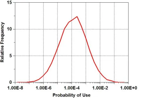
For this model population the RSPF is given by
exp(β0 + 2.0x1 + 1.0x2 + 0.0x3)
W*(x1,x2,x3) = ---
1 + exp(β0 + 2.0x1 + 1.0x2 + 0.0x3)
so X3 is not important for selection and the value of β0 fixes the overall probability of a unit being recorded as
being used by an animal. Fig. 1 shows the function for the particular case where 1000 of the million resource
units are expected to be used.
Fig. 1 Relative probabilities of use for a large sample of resource units when the expected total number of used units is 1,000, i.e., 0.1% of all one million units. Probabilities of use vary from about 10-8 to 0.25, with a mean of 0.001.
For the simulation study the expected number of used units in the population (n1) was set at 50, 100, 200,
400 or 800. For each of these expected values of n1 the sample size for unused units (n2) was set at 1000, 5000
real data many more than 100 bootstrap sets of data would be used so that, if anything, the bootstrap results obtained in the simulation study are not as good as what might be obtained with real data.
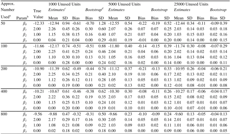
We summarise the bootstrap results in two ways. First, Table 1 shows the true regression coefficients, the mean and standard deviation from 100 generated sets of data, the apparent bias in the estimates, the mean bias estimated by bootstrapping and the mean standard deviation estimated by bootstrapping. Only the results for
parametric bootstrapping are given in this table. As discussed below, this clearly gave better results than nonparametric bootstrapping.
Table 1 Results from generating 100 sets of data for each of 15 scenarios with 50 to 800 resource units expected to be observed to be used and a sample of 1000, 5000 or 25000 unused resource units.
Approx. Number
Useda
1000 Unused Units 5000 Unused Units 25000 Unused Units
True Value
Estimatesc Bootstrapd Estimates Bootstrap Estimates Bootstrap
Paramb Mean SD Bias Bias SD Mean SD Bias Bias SD Mean SD Bias Bias SD 50 β0 -12.33 -12.94 0.94 -0.61 -0.70 1.28 -12.55 0.54 -0.22 -0.19 0.52 -12.44 0.34 -0.11 -0.09 0.39
β1 2.00 2.26 0.45 0.26 0.30 0.60 2.07 0.26 0.07 0.07 0.25 2.03 0.14 0.03 0.03 0.18
β2 1.00 1.15 0.38 0.15 0.16 0.40 1.07 0.21 0.07 0.04 0.20 1.03 0.15 0.03 0.02 0.16
β3 0.00 0.04 0.21 0.04 0.00 0.29 -0.01 0.19 -0.01 0.00 0.20 0.00 0.14 0.00 0.00 0.15
100 β0 -11.66 -12.17 0.74 -0.51 -0.51 0.88 -11.80 0.40 -0.14 -0.15 0.39 -11.74 0.30 -0.08 -0.07 0.29
β1 2.00 2.25 0.41 0.25 0.24 0.46 2.04 0.21 0.04 0.06 0.20 2.02 0.14 0.02 0.03 0.14
β2 1.00 1.10 0.30 0.10 0.13 0.31 1.05 0.16 0.05 0.03 0.16 1.04 0.13 0.04 0.02 0.12
β3 0.00 0.00 0.28 0.00 0.00 0.24 0.02 0.16 0.02 0.00 0.14 0.00 0.10 0.00 0.00 0.11
200 β0 -10.90 -11.39 0.62 -0.49 -0.44 0.74 -11.12 0.37 -0.21 -0.13 0.33 -10.95 0.26 -0.04 -0.06 0.21
β1 2.00 2.25 0.34 0.25 0.21 0.40 2.10 0.19 0.10 0.06 0.17 2.02 0.13 0.02 0.02 0.11
β2 1.00 1.12 0.26 0.12 0.11 0.28 1.05 0.13 0.05 0.03 0.13 1.02 0.09 0.02 0.01 0.09
β3 0.00 0.00 0.19 0.00 0.00 0.21 0.02 0.13 0.02 0.00 0.12 -0.01 0.08 -0.01 0.00 0.08
400 β0 -10.21 -10.67 0.61 -0.46 -0.38 0.62 -10.30 0.30 -0.08 -0.11 0.26 -10.27 0.17 -0.06 -0.04 0.17
β1 2.00 2.22 0.36 0.22 0.19 0.35 2.03 0.17 0.03 0.05 0.15 2.02 0.08 0.02 0.02 0.09
β2 1.00 1.15 0.25 0.15 0.10 0.24 1.01 0.12 0.01 0.03 0.12 1.01 0.07 0.01 0.01 0.07
β3 0.00 0.00 0.20 0.00 0.00 0.19 0.01 0.10 0.01 0.00 0.10 -0.01 0.07 -0.01 0.00 0.06
800 β0 -9.56 -9.88 0.47 -0.32 -0.31 0.50 -9.66 0.23 -0.10 -0.09 0.24 -9.60 0.13 -0.05 -0.04 0.13
β1 2.00 2.17 0.29 0.17 0.16 0.30 2.05 0.14 0.05 0.05 0.14 2.01 0.07 0.01 0.01 0.07
β2 1.00 1.08 0.21 0.08 0.09 0.22 1.03 0.09 0.03 0.02 0.11 1.01 0.06 0.01 0.01 0.06
β3 0.00 0.02 0.18 0.02 0.00 0.18 0.00 0.08 0.00 0.00 0.09 0.00 0.06 0.00 0.00 0.05
a
Data are generated using probabilities of being observed to be used so that the actual number observed to be used is a random variable with the expected value shown
b
The true parameter values used to generate data., which are the same for the three sample sizes of unused units. c
The mean, standard deviation, and mean bias (mean estimate - true value) of estimates from 100 generated sets of data. d
The average estimated bias and the average estimated standard deviation from parametric bootstrapping applied to each of the 100 sets of generated data, with 100 bootstrap sets of data for each generated set of data.
Table 1 shows that the estimated values of the regression constantβ0 have a negative bias which decreases
as the number of unused units increases and as the sample size increases for the unused units. In contrast to
this, the estimates of the non-zero regression coefficients β1 and β2 have positive biases which also decrease as
the number of used units increases and as the sample size for unused units increases. There is, however, little if
any bias in the estimates of the zero coefficient β3. These small sample biases are in the direction of making
selection appear more extreme than it really is.
observed standard deviations of the estimates of regression coefficients with a sample of 1000 unused units and 200 or less used units. Although the estimated regression coefficients show bias it appears that this is
estimated well by parametric bootstrapping, at least on average. Similarly, the observed standard deviations of the estimated regression parameters are close to the mean of the bootstrap estimates when there are more than 1000 unused units or more than 200 used units. The results in Table 1 therefore indicate that the bootstrapping
is effective for estimating and removing biases in estimated regression coefficients and for determining the standard deviations of these coefficients providing that the sample of used units and the sample of unused units
are not both quite small.
If the bootstrap estimates of biases and standard deviations are close to the correct values then inferences about regression coefficients can be based on the assumption that
Zi = (bi - Biasi - βi)/SDi (4)
approximately follows a standard normal distribution, where biis the pseudo-likelihood estimate of the
parameter βi in equation (1), Biasi is the bootstrap estimate of the bias in estimating βi, and SDi is the bootstrap
estimate of the standard deviation of bi. For example, if the normal approximation is valid, it is possible to
construct a 95% confidence interval for βi as
bi - Biasi - 1.96 SDi < βi < bi - Biasi + 1.96 SDi,
while bi is significantly different from zero at the 5% level if (bi - Biasi)/SDi is outside the range from -1.96 to
+1.96.
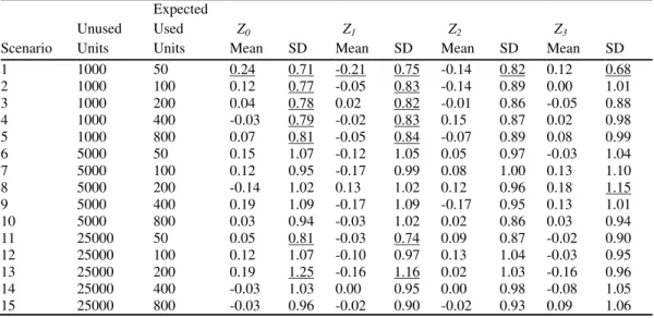
Table 2 Means and standard deviations of the Zi values as defined by equation (4) for the simulation study described in Section 3. Underlined values of the mean are significantly different from zero at the 5% level (outside the range from -0.20 to + 0.20). Underlined values of the standard deviation (SD) are significantly different from one at the 5% level (outside the range 0.86 to 1.14).
Expected
Unused Used Z0 Z1 Z2 Z3
Table 2 indicates that the assumption that the Zi values of equation (4) have means of zero and standard deviations of one is reasonable when the size of the sample of unused units is 5000 or 25000, but not when it is
only 1000. With only a sample of 1000 unused units the simulated standard deviations of the Z values are
usually too low because of the positive bias in the bootstrap estimated standard deviations of the regression
coefficients. With 5000 or 25000 unused units the standard deviation of Z values is significantly different from
one at the 5% level five times but with no clear pattern because three of the five standard deviations are greater
than one and two are less than one. There is little evidence that the means of Z values differ from zero, so that
over all treating Z values as having means of zero and standard deviations of one seems reasonable if the size
of the sample of unused units is at least 5000.
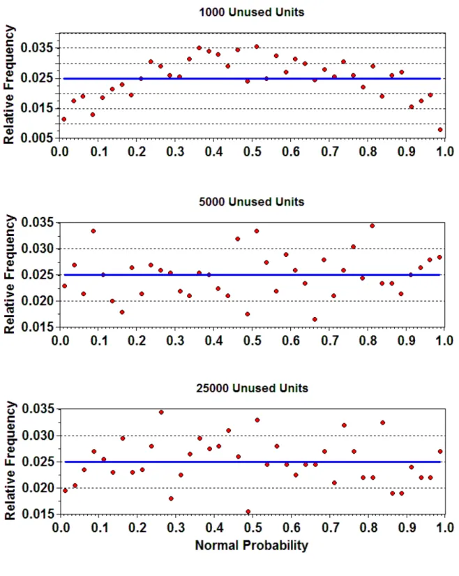
For inferences it is also necessary that the Z values from equation (4) have distributions that are close to
the standard normal distribution. In particular φ(Z) should have a distribution that is close to uniform between
zero and one, where φ(z) is the cumulative normal distribution function. This is not the case with only 1000
unused units samples, but is a good approximation for 5000 and 25000 unused units, as shown by Fig. 2. In
this connection it can be noted that with 1000 unused units the percentage of Z values significantly different
from zero at the 5% level is quite low at 2.0%, but the percentages for 5000 and 25000 are close to the desired
5%, being 5.2% and 4.7%, respectively.
To sum up the results from the simulation experiment, it seems that inferences about estimated regression
coefficients can be based on assuming that they are normally distributed with small sample biases and variances that can be estimated reasonably well by parametric bootstrap resampling, providing that the sample
size for unused units is large enough. For the situations considered in the simulations a sample size of 5000 or more unused units seems to be reasonable. This is consistent with the conclusion of Nielson et al. (2004) that there is little point in using more than 10000 available resource units when estimating a resource selection
function using ordinary logistic regression with a sample of units observed to be used and a random sample from the population of available resource units.
4 Conclusions
There are a number of issues that need to be considered when using the logistic regression method described in
this paper to estimate a resource selection probability function. For example, the method provides an estimate of the probability that resource unit is observed to be used. If not all used units are observed to be used then the
probability being estimated can be interpreted as the probability of a units being used multiplied by the
probability θ that the unit is recorded as being used. If θ is the same for all units then this may be considered to
be acceptable. However, if θ varies according to the nature of the resource unit then the estimated resource
selection probability function is biased in terms of estimating the actual use of resources. We do not consider this issue further here, but note that it can be allowed for using the methods discussed by Mackenzie (2006).
A limitation with assuming a logistic resource selection probability function is that if this is correct for time duration then it cannot be correct for any other time duration. For example, assume that the probability of
a resource unit being recorded as used at least once in one year is w1*(x1,x2,...,xp), where this is a logistic
function of the covariate values x1 to xp measured on the unit. Assume also that the probability of the unit
being recorded as used at least once in a second year is exactly the same, with independence between years. Then the probability of the unit being used at least once in the two year period is
w2*(x1,x2,...,xp) = 1 - {1 - w1*(x1,x2,...,xp)}2
which is one minus the probability that it is not recorded as used in both years. This is not a logistic regression function, showing that the logistic regression assumption cannot hold for both a one year selection period and
a two year selection period unless perhaps the function is not the same in both years.
Although this is true, the logistic function will be a good approximation if the probability of use in one year is small for all resource units. In that case the numerator in the logistic function
exp(β0 + β1x1 + ... + βpxp)
w1*(x1,...,xp) = ---
1 + exp(β0 + β1x1 + ... + βpxp)
will be close to zero and the denominator will be close to one. Also, w1*(x1,...,xp)2 will be negligible in the
equation for w2*(x1,...,xp). Hence
w1*(x1,...,xp) ≈ exp(β0 + β1x1 + ... + βpxp)
and
w2*(x1,x2,...,xp) ≈ 2 exp(β0 + β1x1 + ... + βpxp) = exp{loge(2) +β0 + β1x1 + ... + βpxp}
where both of these functions will be well approximated by logistic regressions.
What this means is that the assumption of a logistic regression for estimating a resource selection probability function will be reasonable providing that all units have small probabilities of use for the time periods of interest. If this is not the case then logistic regression may still give a reasonable empirical
approximation for the true resource selection probability function but it is important to appreciate that the approximation is specific to the time period used for the study. The pseudo-likelihood estimation method
described in this paper can be applied with another form of function that allows for different time periods of selection better, but this has not yet been investigated.
Finally, we note that Lele and Keim (2006) describe a method for estimating a resource selection
probability function based on the idea of a weighted distribution. This method does not require knowledge of the total number of resource units in a population or how many of these were used during the period of a study.
We would have liked to compare the estimates from this method with the estimates obtained by the method we describe here but we were unfortunately not able to get convergence with sets of data of the kind used in out
simulations using the R program provided by Lele and Keim in a Supplement to their paper. We did get
convergence with their data and suspect that the problem is that the Lele and Keim method requires a fairly high proportion of resource units to be used in order to produce estimates. We did generate one set of data for a
population of 100,000 resource units with 9812 used units, i.e. 9.8% used. With data on all of the used units and a sample of 10,000 available units we were still unable to get convergence for the Lele and Keim R
program, which is why we suspect that it requires a fairly high proportion of units to be used.
Acknowledgements
RO acknowledge funding from Conselho Nacional de Desenvolvimento Científico (CNPq). We thank the
References
Keating KA, Cherry S. 2004. Use and interpretation of logistic regression in habitat-selection studies.
Journal of Wildlife Management, 68: 774 -789
Lele SR, Keim JL. 2006. Weighted distributions and estimation of resource selection probability functions. Ecology, 87: 3021-3028
Mackenzie DI. 2006. Modelling the probability of resource use: the effect of, and dealing with, detecting a species imperfectly. Journal of Wildlife Management, 70: 367-374
Manly BFJ. 1985. The Statistics of Natural Selection on Animal Populations. Chapman and Hall, London, UK Manly BFJ, McDonald LL, Thomas DL, et al. 2002. Resource Selection by Animals: Statistical Design and
Analysis for Field Studies. Kluwer, Dordrecht
McCracken ML, Manly BFJ, Heyden MV. 1998. The use of discrete-choice models for evaluating resource selection. Journal of Agricultural, Biological and Environmental Statistics, 3: 268-279
McDonald LL, Manly BFJ, Rayley CM. 1990. Analysing foraging and habitat use through selection functions. Studies in Avian Biology, 13: 325-331
McDonald TL, Manly BFJ, Nielson R, et al. 2006. Discrete choice models with a spotted owl example.
Journal of Wildlife Management, 70: 375-383
Nielson R, Manly BFJ, McDonald LL. 2004. A preliminary study of the bias and variance when estimating a
resource selection function with separate samples of used and available resource units. In: Resource Selection Methods and Applications (Huzurbazar S, ed). Omnipress, 28-34, Madison, Wisconsin, USA Strickland MD, McDonald LL. 2006. Introduction to the special issue. Journal of Wildlife Management, 70:
321-323
Zhang WJ. 2010. Computational Ecology: Artificial Neural Networks and Their Applications. World