Braz. J. of Develop.,Curitiba, v. 6, n. 10, p. 79834-79855, oct. 2020. ISSN 2525-8761
Impact of soy exports from the North on market integration: the case of
Paranaguá and Sorriso
Impacto das exportações de soja do Norte na integração do mercado: o caso de
Paranaguá e Sorriso
DOI:10.34117/bjdv6n10-419
Recebimento dos originais: 15/09/2020 Aceitação para publicação: 20/10/2020
Victor Yoiti Ikeda
Mestre em Economia Aplicada pela Escola Superior de Agricultura "Luiz de Queiroz" Instituição: Universidade de São Paulo. Analista da área agrícola do Rabobank Endereço: Av. Das Nações Unidas, 12.995, 7º. Andar, Brooklin Novo – São Paulo
E-mail: victor.ikeda@rabobank.com Andréia Cristina de Oliveira Adami
Doutora em Economia Aplicada pela Escola Superior de Agricultura "Luiz de Queiroz” Instituição: Universidade de São Paulo. Cepea/ESALQ/USP, Piracicaba
E-mail: adami@cepea.org.br Geraldo Sant’Anna de Camargo Barros PhD em Economia pela North Carolina State University
Professor Sênior da Escola Superior de Agricultura "Luiz de Queiroz” - ESALQ
Coordenador Científico do Centro de Estudos Avançados em Economia Aplicada da ESALQ – Cepea/ESALQ/USP, Piracicaba
E-mail: gscbarro@usp.br ABSTRACT
The aim of this paper was to evaluate the cointegration in the Brazilian soybean markets which could be affected by the alternative export route from the Center-West's production through the Northern ports. According to the hypothesis of this work the soybean-producing region can raise competitiveness due to the export alternative through the ports of the so-called "Northern Arc", once they are closer to the international consumer markets in the Northern Hemisphere. The time-series analysis indicates that the exports through the ‘Northern Arc’ can be considered as one of the factors that raised the level of prices in Sorriso in comparison to Paranaguá. The maintenance of the cointegration relationship between Sorriso and Paranaguá can be justified by the fact that Pará port cannot absorb all the exports from Mato Grosso soybeans, so significant part of Sorriso production is still exported by the ports of the South-Central region.In addition, the concept of export parity presupposes the soybean pricing based in Chicago, regardless of the port used for export.
Key-words: Soybean, Competitiveness, Arco-Norte, transportation cost. RESUMO
O objectivo deste documento era avaliar a cointegração nos mercados de soja brasileiros que poderiam ser afectados pela rota alternativa de exportação da produção do Centro-Oeste através dos portos do Norte. De acordo com a hipótese deste trabalho, a região produtora de soja pode aumentar a competitividade devido à alternativa de exportação através dos portos do chamado "Arco Norte", uma
Braz. J. of Develop.,Curitiba, v. 6, n. 10, p. 79834-79855, oct. 2020. ISSN 2525-8761 vez que estes estão mais próximos dos mercados internacionais de consumo no Hemisfério Norte. A análise da série temporal indica que as exportações através do "Arco Norte" podem ser consideradas como um dos factores que elevaram o nível de preços em Sorriso em comparação com Paranaguá. A manutenção da relação de cointegração entre Sorriso e Paranaguá pode ser justificada pelo facto do porto do Pará não poder absorver todas as exportações de soja de Mato Grosso, pelo que uma parte significativa da produção de Sorriso é ainda exportada pelos portos da região Centro-Sul. Além disso, o conceito de paridade de exportação pressupõe o preço da soja baseado em Chicago, independentemente do porto utilizado para a exportação.
Palavras-chave: Soja, Competitividade, Arco-Norte, custo de transporte
1 INTRODUCTION
This paper aims to analyze aspects related to the pricing of soybeans in the Brazilian domestic market, focusing on factors related to grain-producing location and transport costs. The relevance of this topic stems from the fact that soybeans are one of the main Brazilian export products; however, the production is largely developed in the Center-West, mainly in the state of Mato Grosso, far away from the traditional ports, located in the Center-South of the country. Consequently, there is a strong negative impact on the domestic prices and, therefore, losses of competitiveness given by high local logistical costs.
The hypothesis of this work is that the soybean-producing region can raise competitiveness due to the export alternative through the ports of the so-called "Northern Arc", once they are closer to the international consumer markets in the Northern Hemisphere. According to Morales et al. (2013), the port of Santarém (PA), for example, is located at around five thousand nautical miles closer to the Europe than the Port of Santos (SP). Moreover, such as Costa et al. (2001), this alternative also reduces the transportation of the soybeans; it means that it is not necessary for the soybean produced in a Northern region of Brazil to move towards the South to be exported to a port in the Northern Hemisphere, either in Asia or in Europe. In addition, it allows the use of several types of transportation models as an alternative to exclusively road transport that predominates in the country. As a result, the soybeans transportation cost for exports through the port of Santarém to Europe, for instance, could be from 20% to 30% lower than through the port of Santos.
The exports of soy and corn through the ‘Northern Arc’ had a significant rise in the last years. According to Ikeda (2018), from 2010 to 2017, the volume exported through ports in the North and Northeast regions of Brazil increased by 34.9% to 26.3 million tons. The internal logistics for ‘Northern Arc’ also have distinct logistic network, once 50% of the grains reach the ports via waterways, 22%
Braz. J. of Develop.,Curitiba, v. 6, n. 10, p. 79834-79855, oct. 2020. ISSN 2525-8761 via railways and 28% highways. In the case of Center-South ports, the logistics matrix is composed by 50% road, 49% rail and only 1% waterway.
The local crushing industry’s expansion as well as the development of the animal protein sector in the Brazilian Center-West may be other reason, which boosted the profitability of soybean production in these more internalized producing regions. In terms of local demand for soybeans, it is worth mentioning that the installed oilseed processing capacity in Mato Grosso increased from 20,600 tons/day in 2004 to 41,259 tons/day in 2016, an increase of 100%, according to Abiove (BRAZILIAN ASSOCIATION OF VEGETABLE OILS INDUSTRIES, 2018). In the same period, the herd of poultries (total) in the state increased by 224%, the hog (total) grew by 93% and the cattle had an increase of 17%, according to IBGE (BRAZILIAN INSTITUTE OF GEOGRAPHY AND STATISTICS, 2018).
Thus, there is a perspective of economy on the value of the freight rate from the Mato Grosso’s soybeans exported through the Northern ports in relation to the ports located in the South and Southeast regions of Brazil. Rasmussen and Ikeda (2016) emphasize that there is an expectation that soybeans outflow through ‘Northern Arc’ Ports will show a huge growth in the coming years due to the ‘New Port Regulatory Framework’ released in 2013, which favored private investments in this region. Additionally, they may present capacity expansion higher than the ports in the South and Southeast. The main ports to expand their export capacity between 2015 and 2025 should be those comprising the export corridor by Santarém, Barcarena and Santana.
Once the higher soybeans exports through the North might change transmission of soybean prices, mainly in the Brazilian Center-West, this paper will analyze the possible modification in the price influence of the port of Paranaguá on prices in the main producing region of Mato Grosso. In this study represented by the municipality of Sorriso, it is worth noting that the absence of a time series of soybean prices in Santarém (or other ports in the ‘Northern Arc’) precludes the test considering that region, but a possible change in the transmission of prices between Paranaguá and Sorriso may indicate greater influences of both the local market (such curhsing industry) as well as the 'new' export corridors through the North. In terms of quantitative analysis, this paper aims to verify if there has been any change in the pattern of cointegration between soybean prices in these two markets - Sorriso and Paranaguá - mainly considering the level of the relation between these series. The period analyzed was from 2004 to 2017.
Four further sections will be considered additionally to this introduction. Section two presents the theoretical model, including concepts of price formation as well as the interregional transmission of
Braz. J. of Develop.,Curitiba, v. 6, n. 10, p. 79834-79855, oct. 2020. ISSN 2525-8761 prices, applied to the soybean market. In section three, the Zivot & Andrews methodology (1992) and the Chow (1960) is presented. The vector error correction model (VEC) is used to analyze the decomposition of the variance of the prediction errors and the impulse response function of the variables analyzed. The results and the discussions are in the section four, while the conclusions are in the fifth section.
2 THEORETICAL BACKGROUND
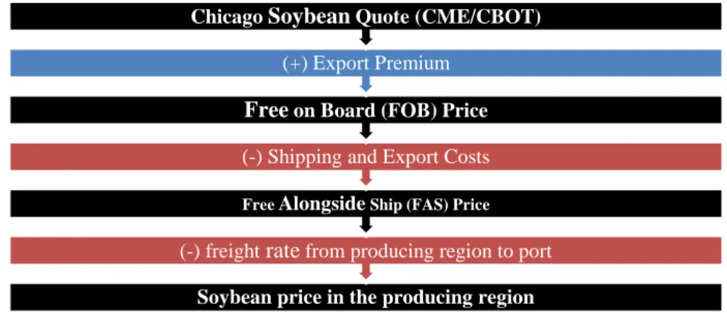
Brazil is still a price taker in the soybean market, even be one of the world's main players in terms of both production and exports (MARGARIDO et al., 1998; MELLO E BRUM, 2020). In other words, soybean prices are determined in the international markets and domestic producers expect that the values practiced internally be in line with those of the external market (BARROS et al., 1997). Cardoso and Waquil (2002) pointed out that the international trade opening, coupled with the reduction of resources applied in the policy of minimum prices in Brazil in the early 2000s, intensified the correlation of the domestic soybean price with the price determined by the Chicago Board of Trade (CME/CBOT). This US commodity futures exchange takes into account in the pricing, among other factors, supply, demand and world grain stocks perspectives (MAFIOLETTI, 2000). Based on the price quoted in the CME/CBOT, premium, port and transportation costs, it is possible to calculate the export parity value in the Brazilian producing regions (Figure 1).
Figure 1 - Soybean export-parity price index based on the Chicago Board of Trade (CME/CBOT) quote for soybeans in the exporting port.
Source: Mafioletti (2000) – prepared by the authors.
In terms of internal price transmission, Moraes (2002) pointed out that the price level in the Brazilian ports, after deducting port costs, freights, etc., results in the price for the processor. From this price, deducting the freight and operational costs, among others, the price received by the farmers at
Soybean price in the producing region
(-) freight ratefrom producing region to port Free AlongsideShip (FAS) Price (-) Shipping and Export Costs
Freeon Board (FOB) Price
(+) Export Premium
Braz. J. of Develop.,Curitiba, v. 6, n. 10, p. 79834-79855, oct. 2020. ISSN 2525-8761 the producing region is obtained. Of course, profits and losses related to logistics and processing may be detected in these calculations. The export parity value may be considered as an indicative of the local price in the Brazilian producing regions. It is worth to mentioning that there are still factors, such as those that characterize the degree of competition in the various market levels, which may result in differences in the value of this indicator when compared to the spot price in a producing region. The marketing involves agents such as brokers, local crushing industry, import and export tradings, cooperatives and buyers of agricultural products, either in cash market or through the crop pledge (CPR).
In theoretical terms, there is the so-called Law of One Price (LOP). According to Krugman and Obstfeld (2005), it means that in a competitive market, in the absence of transport costs and barriers to trade, identical goods sold in different countries can be sold at equal prices when expressed in the same currency. According to Bendinelli et al. (2011), the concept of the LOP can be directly related to the arbitration process, which would guarantee long-term price equilibrium, when expressed as a unit of common value.
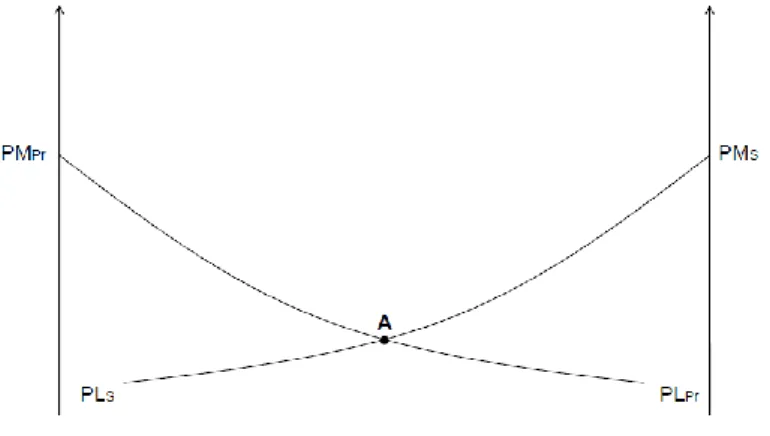
Bressler & King (apud Barros (2011)) presented the theory of competition, in which, if there is trade between two regions, the prices of the goods involved would tend to differentiate on average by the cost of transfer, including the transportation cost in those regions. They defined local price (PL) in a production region as the market price (port, in the case) less the transfer costs involved in placing the product on the market. In addition, when a region, such as Mato Grosso, negotiates in two places, for example in Paranaguá and Santarém, simultaneously, the local prices for each market (port) will be the same. Consequently, in a producing region like Sorriso, it will be indifferent by which port the outflow will take place. Based on Barros (2011), considering that the market is competitive, Figure 2 illustrates the situation: the determination of PL – local prices (per ton) relative to the marketing of a product in two different ports, such as Paranaguá (Pr) and Santarém (S). Each curve has the ordinate of the product (PL) according to the distance to the ports. In this case, transfer costs tend increase at decreasing rates according to the traveled distance, as local prices will tend to fall at decreasing rates as the region is further away from the port. The PLPr curve shows the PL for each production point assuming that the export flow is given by Pr. These would be the prices received by the producer if there was no port of Santarém. In this case, all producers whose costs are covered by the respective PLPr will have their production transferred to Pr.
When there is the possibility of export through Santarém, each region will have two local prices – PLPr and PLS. Assuming that the utilization of the route through Santarém does not affect the price
Braz. J. of Develop.,Curitiba, v. 6, n. 10, p. 79834-79855, oct. 2020. ISSN 2525-8761 in Paranaguá, it is noted that there is a location A in which the two local price curves intersect. In this location, the production can be transferred regardless of any of the ports. It is called the boundary of the Pr and S markets. Now, regions to the right of A will sell their production to S; those on the left will make it to Pr. The regions on the right of A will receive higher prices by sending their production to S. On the left, local prices will remain the same. It is noticed, so that the regions on the right will lose their relationship to Pr and will have it with S. As prices in S and Pr may vary over time, the limit A may oscillate in a transition area and may be linked sometimes to Pr and to S in others. But the areas will tend to be linked to one of the ports in the long term.
Figure 2 - Local prices – PL (per ton in the producing region) relative to the marketing of a product in two different ports considering transfer costs and equal market prices in the ports of Paranaguá (Pr) and Santarém (S).
Source: Barros (2011) – prepared by the authors.
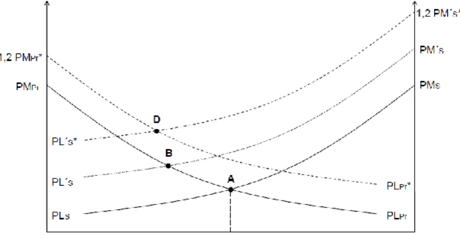
Due to greater proximity to consumer markets of the new export route through Santarém, the price in this port (PM'S) is higher than those observed in Paranaguá, as shown in Figure 3. Considering the same cost functions per kilometer to transfer the grain for both ports, it is observed that the PLPr and PL'S curves intersect at a point B. In this situation two changes can be verified: the area of influence of the Port of Santarém increases, as well as the local price to the producers at the new market limit. It is observed in this case that the producing area that destines its product to S will increase. This results in a higher volume of product exported through the port in S.
In addition to the higher market price in one of the ports, another hypothesis is that with the conclusion of the logistics facilities towards the port of the northern region of Brazil, there may be a change in the transfer costs between the Port of Santarém and the producing regions. This is what can be observed in the PL's curve, in which the slope is lower than that verified in PLPr (indicating lower
Braz. J. of Develop.,Curitiba, v. 6, n. 10, p. 79834-79855, oct. 2020. ISSN 2525-8761 price at the market limit, at point C, between ports, as well as an increase in the area that would send its production to the port of Pará.
Figure 3 - Local prices – PL (per ton in the producing region) relative to the marketing of a product in two different ports considering changes in the cost of transfer and market price in the port of Santarém (S).
Source: Barros (2011) – prepared by the authors.
In Figure 4, the points A and B, are comparing with the D point resulting from equal relative changes (percentages) in the prices of the two ports. The results of a 20% increase in the market prices of Santarém and Paranaguá, taking into account a higher value in the port of Pará (PM'S) and equals
transfer costs, are the PL'S* and PLPR* curves. In this situation, the market limit is represented by point
D, with price higher than point B and increase in the influence area of Santarém. In the case, what happened was that the prices in the ports were different, with higher PLS (and lower transportation
costs); with that the absolute rise was higher in Santarém.
Figure 4 - Local prices – PL (per ton in the producing region) relative to the marketing of a product in two different ports considering similar changes in the market price in the port of Santarém (S) and Paranaguá (Pr).
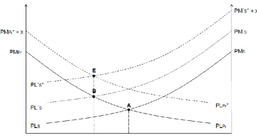
Braz. J. of Develop.,Curitiba, v. 6, n. 10, p. 79834-79855, oct. 2020. ISSN 2525-8761 An alternative scenario considers equal absolute changes in the two ports represented by an increase of x-monetary units in the prices in Paranaguá (PMPR* + x) and Santarém (PM'S*+ x). In this
situation, such as it is represented in the Figure 5 by the PLPR* and PLS* local price curves, it is verified
that there is no increase in the influence area of the port of Santarém, maintaining the location of the market limit (point E, representing the same local than point B), however, there is an increase in the local price in this region.
Figure 5 - Local prices – PL (per ton in the producing region) relative to the marketing of a product in two different ports considering absolute changes equal in the market price in the port of Santarém (S) and Paranaguá (Pr)
Source: Barros (2011) – prepared by the authors.
Given these characteristics of the market, the hypothesis to be tested in this paper is that, even considering the entrance of a new export route, in this case represented by Santarém (S), the prices cointegration between Mato Grosso and Paranaguá (Pr) remained unchanged in the period. Theoretically, this result would indicate that the transition area remains large enough to export its production at both ports. In addition, the concept of export parity presupposes pricing based in Chicago, regardless of the port used for export.
To analyze the price relationship between Sorriso (Ps) and Paranaguá (Pp), it was considered
the model of margins suggested by Gardner (1975, apud BARROS, 2011). The difference is represented by F (simplified as the freight rate):
𝐹 = 𝑃𝑝− 𝑃𝑠 (1)
Consequently, the freight rate as proportion of PP will be represented as:
𝐹
𝑃𝑝 = 1 − 𝑃𝑠 𝑃𝑝
Braz. J. of Develop.,Curitiba, v. 6, n. 10, p. 79834-79855, oct. 2020. ISSN 2525-8761 Gardner (1975, apud BARROS, 2011) defines margin (M) as being the relation between the sale price and the purchase price:
𝑀 = 𝑃𝑝 𝑃𝑠
(3)
Once, M and F move in the same direction, it means 𝑑𝐹
𝑑𝑀> 0, it is possible to define that M is
formed through the equation:
𝑀 = 𝛼𝑃𝑝𝛽 (4) Or, ln 𝑀 = ln 𝛼 + β ln 𝑃𝑝 (5) As well as, 𝑃𝑝 𝑃𝑠 = 𝛼𝑃𝑝 𝛽 (6) Or even by, 𝑃𝑠 = 𝑃𝑝 1−𝛽 𝛼 (7) And in logarithms: ln 𝑃𝑠 = − ln 𝛼 + (1 − 𝛽) ln 𝑃𝑝 (8)
In (8), there is the equation of price transmission from Paranaguá to Sorriso. This transmission would be a result of a mechanism that, given a variation in PP, it is transfered to M with a β-elasticity
or PS with a (1 - β)-elasticity. This elasticity is generally greater than unity since freight is relatively
more stable than commodity prices. Therefore, PS can rise by more than PPR, in percentage terms, in
face of an absolute increase in PPR. In absolute terms, the Sorriso price is obtained, on average,
according to the expression (7): PP is raised to (1 - β) and the result is divided by α.
Equation (8) can be estimated if there is a cointegration between these variables. In the short-term there may be differences in this relationship, but they are corrected over the long run. In the analysis of (8), it is important to test if (1 - β) differs statistically from the unit, this condition is relevant to evaluate whether the margin is influenced by PP. It is important to check if there are structural breaks
in the intercept (level), which could be associated with changes in the pricing due, for instance, to the a ‘new’ export flow through the North region, i.e. in the example analyzed in this paper could be the Santarém influence.
Braz. J. of Develop.,Curitiba, v. 6, n. 10, p. 79834-79855, oct. 2020. ISSN 2525-8761 3 METHODOLOGY
3.1 DATA
The time series used in this paper were soybean prices in the spot market in Sorriso and the ESALQ/BM&F Bovespa Soybean Index for Paranaguá, calculated by the Center for Advanced Studies on Applied Economics from Department of Economy, Sociology and Administration at Luiz de Queiroz College of Agricultura (ESALQ), from the period of January 2004 to December 2017. The data were considered in dollars (US$/60kg bag) in a daily basis. It is worth to mentioning that there were not considered information from days when there was no business due to local holidays in one of the regions. The ESALQ/BM&F Bovespa Soybean Index for Paranaguá refers to the value of soybean delivered at place or free alongside ship in the warehouse at the port and delivered at the unit that loads ships at Paranaguá port, without taxes. This indicator is used to the financial liquidity of future soybean contract at BM&F Bovespa.
The municipality of Mato Grosso used for the analysis was Sorriso, the largest soybean producer of Mato Grosso (IBGE, 2018). Morales et al. (2013) indicate that this municipality is located strategically in the central area of the state and, for this reason, it can be considered as the potential area of influence for the production flow from the North of Mato Grosso to the port of Santarém. This region is also expected to expand rapidly in the next few years due to the possibility of exports through the ‘Northern Arc’ ports (RASMUSSEN AND IKEDA, 2016).
3.2 UNIT ROOT TEST WITH STRUCTURAL BREAK
In order to evaluate the behavior of the relationship between the two series, the unit root test with structural break was used over the complete series of the relative margins (yt) between the Sorriso
and Paranaguá regions. This test determined two subperiods to be considered in the cointegration analysis. The objective was to verify if there was a potential point that could change the stationarity level of the relative margins’ series. The aim of this test was to check whether there was a change in the average in which the series remains stationary. Thus, to evaluate some moment in which there may have been a change in transmission prices from Paranaguá to Sorriso region.
Zivot and Andrews (1992) based on the Perron’s methodology (1989) developed a test in which they proposed as a change, the fact that the Dummy variable referring to the moment of the break can be endogenous, not exogenous. The authors proposed to make this endogenous (breaking) variable, allowing the analysis to be performed without knowing the point of structural break; it is, therefore, a dynamic test. Based on the Perron’s methodology (1989) and considering the breaking point as an
Braz. J. of Develop.,Curitiba, v. 6, n. 10, p. 79834-79855, oct. 2020. ISSN 2525-8761 endogenous factor to the series, the authors elaborated new statistical tests, starting from the following models:
𝑀𝑜𝑑𝑒𝑙 𝐴: 𝑦𝑡= 𝜇1+ 𝛽𝑡+ (𝜇2− 𝜇1)𝐷𝑈𝑡+ 𝑒𝑡 (9)
𝑀𝑜𝑑𝑒𝑙 𝐵: 𝑦𝑡 = 𝜇1+ 𝛽1𝑡 + (𝛽2− 𝛽1)𝐷𝑇𝑡+ 𝑒𝑡 (10) 𝑀𝑜𝑑𝑒𝑙 𝐶: 𝑦𝑡 = 𝜇1+ 𝛽𝑡+ (𝜇2− 𝜇1)𝐷𝑈𝑡+ (𝛽2− 𝛽1)𝐷𝑇𝑡+ 𝑒𝑡 (11)
Perron (1989) denominates the model A as the "shock model" because it estimates the change in the level of the series signaled by (𝜇2− 𝜇1), which indicates the change in the intercept. The model B indicates the change in the slope at a certain point of the structural break and this change is given by (𝛽2− 𝛽1). The model C combines both the level and the slope changes of the time series. DU is the dummy variable that assumes value 1 from the moment of the shock and it is used to capture the change at the series level and DT is the dummy variable used to capture the effect on the slope. Given this information, the null hypothesis for Zivot and Andrews (1992) is:
𝑦𝑡 = 𝜇 + 𝑦𝑡−1+ 𝑒𝑡 (12)
From the null hypothesis defined in (12), Zivot and Andrews (1992) estimate again the three models with the objective of estimating the structural break point that gives the highest weight to the alternative stationary trend. Thus, the proposed test is a unit root test against the stationarity alternative with structural break at some unknown point, without adopting a subjective procedure of choice. Therefore, it is not necessary to use the dummy variable used by the Perron methodology (1989). The authors estimate the ADF test for the presence of unit root and the structural break point is designated as the one that presents the lowest "t" statistic for the ADF test. Thus, the break date is chosen at points where there is evidence less favorable to the null hypothesis of unit root. The endogenous break test is indicated for the case of this study because it is difficult to define with certainty the moment when the volume of operations was enough to alter the margins of the grains marketing. However, the volume exported through Santarém, and also by the other ports of the so-called ‘Northern Arc’, has grown significantly in the recent years (Rasmussen & Ikeda, 2016), so the Zivot and Andrews (1992) test may indicate the point, from which a certain volume may have been sufficient to change the marketing relation, that point is unknown, but can be identified by that test.
Braz. J. of Develop.,Curitiba, v. 6, n. 10, p. 79834-79855, oct. 2020. ISSN 2525-8761 3.3 CHOW TEST
From the results of the test of Zivot and Andrews (1992) were considered two periods of analysis, in which the Chow Test (1960) was applied. A linear regression model was fitted to the data for the two distinct time series. The aim of this linear regression model was to verify if the estimates of the coefficients of the analyzed periods could be considered stable.
This test assumes that the errors of the two regressions (with sample sizes 𝑛1 and 𝑛2) are independent and identically distributed with normal distribution. The first step is to adjust a linear regression by combining the two samples that will have the dimension 𝑛 = 𝑛1+ 𝑛2. From the results of this regression there is obtained the sum of the squares of the residue, called 𝑆1. The degrees of
freedom will be given by 𝑛1+ 𝑛2− 𝑘, in which k represents the number of estimated parameters including the intercept. The second step consists in adjust regressions for each of the periods considered with dimensions 𝑛1 and 𝑛2. Consequently, two square sums of the residues (𝑆2 and 𝑆3) are obtained. For this evaluation are considered 𝑛1+ 𝑛2− 2𝑘 degrees of freedom.
After these two steps, a test 𝐹(𝑘,𝑛1+𝑛2−2𝑘) is performed as follows:
𝐹 = [𝑆1− (𝑆2+ 𝑆3)]/𝑘 [(𝑆2+ 𝑆3)/(𝑛1+ 𝑛2− 2𝑘)]
(13)
If the value of the F-statistic found is higher than the critical values tabulated from Fisher-Snedecor's F distribution, the null hypothesis that ‘the coefficient estimates for the two periods are stable’ is rejected.
3.4 THE VECTOR ERROR CORRECTION (VEC) MODEL
Non-stationary series can be co-integrated. They must present the same order of integration. When this occurs, it is necessary to employ an error correction (VEC) model, once co-integrated series have stable long-term equilibrium, which is eliminated with the differentiation process. VEC model maintains the dynamics of convergence between the series in the long-term horizon considering the long-term equilibrium. According to Enders (2004), the choice for the VEC model depends on the stationarity tests and the number of co-integration relationships found. If the number of co-integration ratios (h) is less than the number of variables (n) and greater than zero, i.e. 0 <h <n, the VEC model is the most appropriate to model the variables considered in the analysis, which compose the vector of variables of the model, 𝑋𝑡. The co-integration test used in this paper was developed by Johansen (1988).
Braz. J. of Develop.,Curitiba, v. 6, n. 10, p. 79834-79855, oct. 2020. ISSN 2525-8761 A general VEC model has the following format:
𝛥𝑋𝑡 = 𝜃 + Γ1𝛥𝑋𝑡−1+ Γ2𝛥𝑋𝑡−2+ ⋯ + Γp−1𝛥𝑋𝑡−𝑝−1+ πXt−1+ εt (14)
Where: 𝛥𝑋𝑡 = 𝑋𝑡− 𝑋𝑡−1; 𝜃 is the parameter referring to the constant considered in the model;
𝜋 = 𝛼𝛽′ is a matrix (𝑛𝑥𝑛), where: (a) α is the adjustment matrix and presents the rate in which the elements 𝑋𝑡 (variables considered in the model) adjust in response to the lagged deviations, considering the cointegration ratios (ℎ); (b) β' is a co-integration vector (ℎ𝑥𝑛), which represents the n transformed series and the co-integration relationships (ℎ).
According to Enders (2004), it is possible to build a model with n-equations, where each equation contains 𝑝 lags (number of temporal lags) of all n variables of the system. To determine the appropriate lag, one criterion is to use multivariate generalizations of the AIC (Akaike information criterion) and SBC (Schwarz Bayesian Criterion) tests. The selected model will be the one that minimizes AIC and SBC values.
Based on the results of these tests applied to soybean prices in Sorriso and Paranaguá in the two periods considered, it will be verified if there was a change in the influence of Paranaguá's prices on Sorriso. The impulse response function and the variance decomposition, products of error corrected vector (VEC) model are also analyzed in this paper.
The impulse-response function allows to identify in how many periods a variable converges to its initial average or another stable level after the simulation of a shock in an explanatory variable. In the present article, the impacts are expressed in terms of impulse elasticity (BARROS, 1991 apud MARGARIDO et al., 2001), calculated by dividing the impacts by the standard deviation of the error of the variable that suffers the shock, in this case, the price of soybean in the producing region, by the standard deviation of the variable that causes the shock, in this case, the price in the port. To apply the term elasticity, the variables must be expressed in logarithms.
The decomposition of the variance of prediction errors is also an important tool of the VAR/VEC models. This indicates the proportion of the variance of prediction errors in each series that is explained due to its own shocks and other variables (ENDERS, 2004). It is possible to decompose the variance of the forecast error n-steps forward in proportions according to shocks in the system variables. Thus, again analyzing the two periods considered, it can be verified if there was any change in the price interaction between Paranaguá and Sorriso through the analysis of the decomposition of the variance of prediction errors.
Braz. J. of Develop.,Curitiba, v. 6, n. 10, p. 79834-79855, oct. 2020. ISSN 2525-8761 4 RESULTS AND DISCUSSION
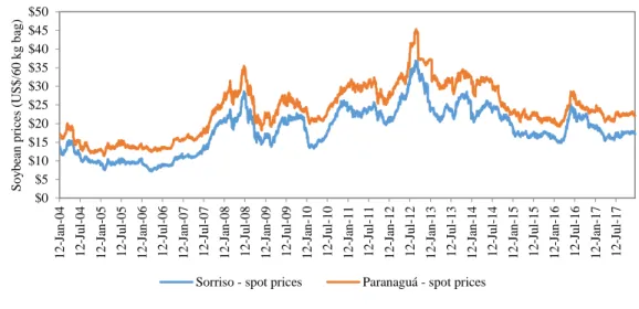
The Figure 6 shows the series of nominal soybean prices in the spot market (US$/60kg bag) in Sorriso and Paranaguá. Confirming aspects quoted in the literature review on oilseed pricing, the values in the port are higher than those in the Mato Grosso region throughout the period. The absolute difference between prices in Paranaguá and Sorriso represents simplified the freight rate (F = Price Paranaguá - Price Sorriso).
Figure 6. Historical (nominal) soybean prices in the spot market (US$/60kg bag) in Sorriso and Paranaguá from 2004 to 2017.
Source: Cepea (2018) – prepared by the authors.
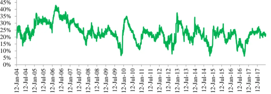
The relative difference between the prices in Sorriso and Paranaguá in the period from 2004 to 2017 is presented in the Figure 7. The values presented represent the percentage difference between the prices in these two regions, M '= F / PR. It can be observed that the series has a huge variability, since it is a daily series. Still, between 2004 and 2007 there is a concentration of higher values, around 30%, suggesting that there may indeed have been a change in the level of the series after 2007, indicating that the difference between prices in the two regions was lower after the increase in the volume of operations through the Northern Arc ports.
$0 $5 $10 $15 $20 $25 $30 $35 $40 $45 $50 1 2 -Ja n -0 4 1 2 -Ju l-0 4 1 2 -Ja n -0 5 1 2 -Ju l-0 5 1 2 -Ja n -0 6 1 2 -Ju l-0 6 1 2 -Ja n -0 7 1 2 -Ju l-0 7 1 2 -Ja n -0 8 1 2 -Ju l-0 8 1 2 -Ja n -0 9 1 2 -Ju l-0 9 1 2 -Ja n -1 0 1 2 -Ju l-1 0 1 2 -Ja n -1 1 1 2 -Ju l-1 1 1 2 -Ja n -1 2 1 2 -Ju l-1 2 1 2 -Ja n -1 3 1 2 -Ju l-1 3 1 2 -Ja n -1 4 1 2 -Ju l-1 4 1 2 -Ja n -1 5 1 2 -Ju l-1 5 1 2 -Ja n -1 6 1 2 -Ju l-1 6 1 2 -Ja n -1 7 1 2 -Ju l-1 7 S o y b ea n p ri ce s (U S $ /6 0 k g b ag )
Braz. J. of Develop.,Curitiba, v. 6, n. 10, p. 79834-79855, oct. 2020. ISSN 2525-8761
Figure 7 - Evolution of the relative margin (%) of prices (US$/60kg bag) in Sorriso and Paranaguá from 2004 to 2017
Source: Cepea (2018) – prepared by the authors.
The structural break analysis was applied to the relative price differentials between the values in Sorriso and Paranaguá using the Zivot and Andrews (1992) test to verify only the model that indicates potential change in the level (intercept) of the series (Table 1). The estimated values lead to the rejection of the unit root hypothesis in the relative margin series at the 10% and 5% level of significance, because in these two cases, the value of the test is lower than the critical values. The point 800, referring to March 2007 is pointed out as a potential structural break point at the series level.
Table 1 - Zivot and Andrews Test (1992) of unit root with structural break in the relative differentials of soybean prices between Sorriso and Paranaguá from January 2004 to December 2017.
Model
Test-Value
Critical values H0: existence of unit root
Potential Strucutural-Break Point
1% 5% 10%
Potential change in the level
(intercept) of the series -5.10 -5.34 -4.80 -4.58 Rejected 800 Source:: Research findings.
Considering the period before the potential structural break point indicated, the average of the relative difference between port (Paranaguá) and producing region (Sorriso) is 29.6%. For the second period, from April 2007 to December 2017 the average is 21.4%. In this case, it is worth to mentioning that this reduction in the average-difference between Sorriso and Paranaguá considering as reference the potential structural break point at the series level. For the purposes of the following analyzes, therefore, two periods will be considered in the sample, the first one being prior to March 28, 2007 (point 800) and the subsequent one.
Before the application of the stability test of the coefficients of Chow (1960), a linear regression model was adjusted with the price of the soybean in Sorriso (PS) as dependent variable and the price in
Paranaguá (PP) as explanatory variable, considering the data from the first period (prior to March 2007). 0% 5% 10% 15% 20% 25% 30% 35% 40% 45% 50% 1 2 -Ja n -0 4 1 2 -Ju l-0 4 1 2 -Ja n -0 5 1 2 -Ju l-0 5 1 2 -Ja n -0 6 1 2 -Ju l-0 6 1 2 -Ja n -0 7 1 2 -Ju l-0 7 1 2 -Ja n -0 8 1 2 -Ju l-0 8 1 2 -Ja n -0 9 1 2 -Ju l-0 9 1 2 -Ja n -1 0 1 2 -Ju l-1 0 1 2 -Ja n -1 1 1 2 -Ju l-1 1 1 2 -Ja n -1 2 1 2 -Ju l-1 2 1 2 -Ja n -1 3 1 2 -Ju l-1 3 1 2 -Ja n -1 4 1 2 -Ju l-1 4 1 2 -Ja n -1 5 1 2 -Ju l-1 5 1 2 -Ja n -1 6 1 2 -Ju l-1 6 1 2 -Ja n -1 7 1 2 -Ju l-1 7
Braz. J. of Develop.,Curitiba, v. 6, n. 10, p. 79834-79855, oct. 2020. ISSN 2525-8761 The result is given by: PS = -0.9831 + 1.2366PP, with standard errors of the coefficients of 0.0253 and
0.0673, respectively, and R2=0.7496. PS is the logarithm of the price in Sorriso and PP is the logarithm
of the price in Paranaguá. In terms of the economic model, as shown above, the estimates of the function: : 𝑃𝑃
𝑃𝑆 = 𝛼𝑃𝑃
𝛽
are given by 𝛼 = 𝑒0.9831 ≅ 2.67 and 𝛽 = 1 − 1.2366 = −0.2366 for period
from January 2004 to March 2007.
Therefore, considering the average-price in Paranaguá in the period under review 𝑃𝑃 = 𝑈𝑆$ 14.35, as 𝑃𝑃𝛽 = 14.35−0.2366= 0.5325 , so 𝑃𝑃
𝑃𝑆 = 2.67 ∗ 0.5325 = 1.4218. It means that the
corresponding price in Sorriso would be 𝑃𝑆 = 𝑃𝑃
1.4218=
14.35
1.4218= 𝑈𝑆$ 10.09. This value compares with
the observed average of 𝑃𝑠 = 𝑈𝑆$ 10,13. It is also noted that the price elasticity of Paranaguá and
Sorriso is (1 − 𝛽) = 1.2366, statistically greater than one. Then, in the first period, a 10% increase in Paranaguá would result in an increase of approximately 12.4% in the price in Sorriso.
In the second period, the result of the regression model is: PS = -0.4815 + 1.0735PP, with
standard deviations 0.0020 and 0.0062, respectively, and R2 = 0.918.
Likewise, in terms of the economic model, the estimates of the function 𝑃𝑃
𝑃𝑆 = 𝛼𝑃𝑃
𝛽
are given by: 𝛼 = 𝑒0.4815≅ 1.62 e 𝛽 = 1 − 1.0735 = −0.0735.
Consequently, if it is considered the average price in Paranaguá in the period 𝑃𝑃 = 𝑈𝑆$ 26.32,
then as 𝑃𝑃𝛽 = 26.32−0.0735= 0.7864 , so 𝑃𝑃
𝑃𝑆 = 1.62 ∗ 0.7864 = 1.2739 . It means that the
corresponding price in Sorrisoe would be 𝑃𝑆 = 𝑃𝑃
1.2739=
26.32
1.2739= 𝑈𝑆$ 20.66. This value compares with
the observed average of 𝑃𝑠 = 20.76.
Please note that the price elasticity from Paranaguá to Sorriso is (1 − 𝛽) = 1.0735, statistically higher than one. Then, in the second period, a 10% increase in Paranaguá would result in a 10.7% increase in the price in Sorriso.
Interestingly, estimates of the long-run equilibrium regression coefficients showed different price elasticity (1-β) in both periods, with a elasticity closer to 1 in the most recent period. In this sense, the Chow test was performed to evaluate if the coefficients of the calculated long-term relationship are statistically stable.
For the Chow test, it was generated the F-statistic considering 2 degrees of freedom in the numerator (with intercept) and 3.471 (800 + 2,671 - 2 * 2) degrees of freedom in the denominator. Next, Table 2 presents the test results with the generated F-statistic and respective critical values at 10%, 5% and 1%.
Braz. J. of Develop.,Curitiba, v. 6, n. 10, p. 79834-79855, oct. 2020. ISSN 2525-8761
Table 2 - Chow's test evaluating stability of linear regression coefficient estimates for the two periods
F-statistic Critical values p-value
10% 5% 1%
224 2.300 3.000 4.610 1.79*10-9
Source: Research findings.
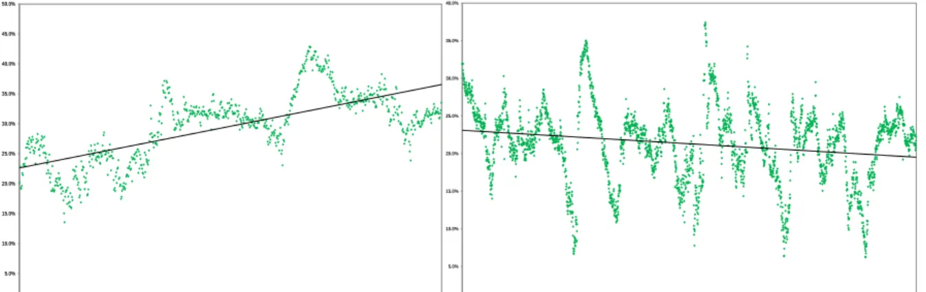
The F-statistic resulting from the Chow test presented a value higher than the critical values. Therefore, the null hypothesis that the coefficient estimates are equal is rejected. This means that the coefficients in the price transmission equations in the two periods are statistically different. Visual examination suggests that these margins showed a negative trend in the second period (Figure 9).
Figure 8 - Evolution of the relative price difference between Sorriso and Paranaguá over time in the first period (January/2004 to March/2007) and the second period (April/2007 to December/2017) and respective trends
Source: Research findings.
From the application of the error correction model in the prices logarithms in Sorriso (PS) and
Paranaguá (PP), the impulse response function and the variance decomposition were obtained. The error
correction model (VEC) was adjusted because the unit-root Dickey-Fuller test indicated that the series have a stochastic tendency, it means, they have a unit root; and the Johansen co-integration test indicated the existence of a co-integration vector between the series. From the error correction model, it was obtained the impulse response function and the impulse elasticities, which are presented in the Figure 9. The chart shows that the price-elasticity transmission from Paranaguá to Sorriso for the first period of analysis is less than unity in the first three days, but then becomes virtually equal to unity from the fourth day.
January 2004 to March 2007 April 2007 to December 2017
0.0% 5.0% 10.0% 15.0% 20.0% 25.0% 30.0% 35.0% 40.0% 45.0% 50.0% 1 1223344556677889100111122133144155166177188199210221232243254265276287298309320331342353364375386397408419430441452463474485496507518529540551562573584595606617628639650661672683694705716727738749760771782793 0.0% 5.0% 10.0% 15.0% 20.0% 25.0% 30.0% 35.0% 40.0% 1316191121 1 5 1 1 8 1 2 1 1 2 4 1 2 7 1 3 0 1 3 3 1 3 6 1 3 9 1 4 2 1 4 5 1 4 8 1 5 1 1 5 4 1 5 7 1 6 0 1 6 3 1 6 6 1 6 9 1 7 2 1 7 5 1 7 8 1 8 1 1 8 4 1 8 7 1 9 0 1 9 3 1 9 6 1 9 9 1 1 0 21 1 0 51 1 0 81 1 1 11 1 1 41 1 1 71 1 2 01 1 2 31 1 2 61 1 2 91 1 3 21 1 3 51 1 3 81 1 4 11 1 4 41 1 4 71 1 5 01 1 5 31 1 5 61 1 5 91 1 6 21 1 6 51 1 6 81 1 7 11 1 7 41 1 7 71 1 8 01 1 8 31 1 8 61 1 8 91 1 9 21 1 9 51 1 9 81 2 0 11 2 0 41 2 0 71 2 1 01 2 1 31 2 1 61 2 1 91 2 2 21 2 2 51 2 2 81 2 3 11 2 3 41 2 3 71 2 4 01 2 4 31 2 4 61 2 4 91 2 5 21 2 5 51 2 5 81 2 6 11 2 6 41 2 6 71
Braz. J. of Develop.,Curitiba, v. 6, n. 10, p. 79834-79855, oct. 2020. ISSN 2525-8761 Figure 9 - Impulse elasticity, referring to the impulse response function, of a shock in the variable PP - logarithm
of the daily price of soybean (US$/60kg bag) in Paranaguá - first period (January 2004 to March 2007)
Source:: Research findings.
In addition to the impulse elasticity analysis, it was verified the decomposition of the prediction error variance, as shown in Table 3.
Table 3 - Decomposition of the variance of the prediction errors of the logarithm of soybean prices in Paranaguá (PP) and Sorriso (PS) - first period (January 2004 to March 2007)
Period Series Variation in Ps Variation in Pp Ps Pp Ps Pp 1 0.765 0.235 0.000 1.000 2 0.636 0.364 0.001 0.999 3 0.554 0.446 0.001 0.999 4 0.497 0.503 0.000 1.000 5 0.466 0.534 0.000 1.000 6 0.441 0.559 0.000 1.000 7 0.422 0.578 0.000 1.000 8 0.406 0.594 0.000 1.000 9 0.393 0.607 0.000 1.000 10 0.380 0.620 0.000 1.000
Source: Research findings.
It is interesting to note that variations in Paranaguá are fully explained due to their own shocks, with 100% influence in the horizon of 10 days. Analyzing, however, the variation in PS it is observed
that in an initial moment they are explained in 75% by the shocks in the series itself in Sorriso, but while the horizon of analysis is extended, the series of Paranaguá starts to exercise each higher influence on the price movements of the series in the region of Mato Grosso, reaching levels above 60% in a period of 10 days. 0 0,2 0,4 0,6 0,8 1 1,2 1 2 3 4 5 6 7 8 9 10 Ps Pp
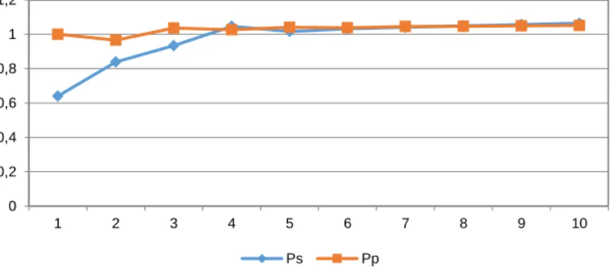
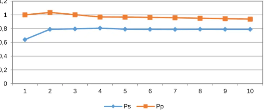
Braz. J. of Develop.,Curitiba, v. 6, n. 10, p. 79834-79855, oct. 2020. ISSN 2525-8761 By evaluating the second period, the elasticity of the impulse (Figure 10) obtained from the impulse response function in the first days is less than unity, increases in the following days, but remains less than unity until stabilized. It might be noted, however, that the evolution of the variable that causes the shock (PP) shows a declining trend.
Figure 6 – Impulse elasticity, referring to the impulse response function, of a shock in the variable PP - logarithm of the daily price of soybean (US$/60kg bag) in Paranaguá - second period (April 2007 to December 2017)
Source:: Research findings.
In this second period, the decomposition of the variance of the prediction errors (Table 4) shows that the movements in the series of Paranaguá (PP) are almost completely explained by their own
shocks. The behavior of the series in Sorriso (PS) is similar to that verified in the previous analysis.
The movements in the first periods are explained by shocks in the producing region (67%), but when the horizon of analysis is extended, it is verified that the series of Paranaguá (PP) has a greater influence
on the price movements of series in the region of Mato Grosso, reaching 51% in 10 days.
These analyzes suggest that there may indeed have been a change in Sorriso's pricing after the intensification of exports by Santarém. The analysis of variance decomposition shows that there is a relative reduction in the influence of Paranaguá over the price changes in Sorriso, however, its relevance remains high. Through the analysis of impulses, the price changes in Paranaguá are no longer transmitted integrally (unit elasticity) to Sorriso, but at around 80%. This means that in the second period, the prices of Sorriso do not suffer the same oscillations as those of Paranaguá, i.e. they have become less volatile. As previously discussed, there are indications that the prices differences have decreased in percentage terms, it means that the two prices approached while the volatility in Sorriso has also reduced.
0 0,2 0,4 0,6 0,8 1 1,2 1 2 3 4 5 6 7 8 9 10 Ps Pp
Braz. J. of Develop.,Curitiba, v. 6, n. 10, p. 79834-79855, oct. 2020. ISSN 2525-8761
Table 4 - Decomposition of the variance of the prediction errors of the logarithm of soybean prices in Paranaguá (PP) and Sorriso (PS) - second period (April 2007 to December 2017)
Period Series Variation in Ps Variation in Pp Ps Pp Ps Pp 1 0.703 0.297 0.000 1.000 2 0.630 0.370 0.003 0.997 3 0.597 0.403 0.003 0.997 4 0.575 0.425 0.005 0.995 5 0.564 0.565 0.007 0.993 6 0.555 0.445 0.009 0.991 7 0.548 0.452 0.010 0.990 8 0.542 0.458 0.011 0.989 9 0.537 0.463 0.013 0.987 10 0.532 0.468 0.015 0.985
Source:: Research findings.
5 CONCLUSIONS
This paper showed interesting points regarding the relation of soybean prices between Sorriso and the port of Paranaguá. Considering the relative price difference between these two regions, a potential breakpoint at the level of this series in March 2007 was identified by structural break test. There was also a change in the price differential between the port and the soybean producing region. In the first period, it was found that the price in Sorriso remained around 30% below the price of the port. For the second period, this relative difference reduced to a level close to 22%. The Chow test on the coefficients of the long-term relations of the two periods confirmed statistically this change.
The price relationships between Sorriso and Paranaguá were also examined through VEC model once the series in the two periods presented a co-integration vector. The variance decomposition indicated that shocks in the Paranaguá price, after ten days, explained 62% of the price changes in Sorriso in the first period (before the structural break). This share fell to 47% in the analysis of the second period. The analyzes of the elasticities of the impulses confirm this change, since in the first period shocks in Paranaguá were integrally transmitted to Sorriso and, in the second period, this transmission drops to levels close to 80%. The changes in the price relationships between Sorriso and Paranaguá may evidence two aspects: strengthening of local demand and impacts caused by the insertion of new export routes, and improvements in the infrastructure of export route from the producing region to the ‘Northern Arc’ports, in particular Santarém. In this case, it was observed that the price level in Sorriso approached in proportion to that of Paranaguá.
The year 2007, which included the potential structural break point was the one in which the port of Santarém had the largest share in the exports of Mato Grosso soybean, during the analyzed period.
Braz. J. of Develop.,Curitiba, v. 6, n. 10, p. 79834-79855, oct. 2020. ISSN 2525-8761 Thus, the new route for the export-flow of production can be considered one of the factors that raised the level of local prices in the producing region. The fact that the prices of Sorriso and Paranaguá remain co-integrated in the second period, even with the change in the transmission ratio, can be justified by the fact that the port of Pará and those of the North in general have not yet been able to absorb all exports of Mato Grosso soybean. Therefore, a significant part of the Mato Grosso (and Sorriso region) business is still carried out by the ports of the Center-South region. Basically, it would be as if the region of Sorriso was at the market limit, maintaining integration of prices with both ports. Producers in regions such as Sorriso already benefitted from alternative export flows and regional demand, as evidenced by the lower relative price difference with Paranaguá. This trend may strengthen as the logistic infrastructure as well as the local market solidify.
REFERENCES
ASSOCIAÇÃO BRASILEIRA DAS INDÚSTRIAS DE ÓLEOS VEGETAIS. Pesquisa de Capacidade Instalada da Indústria de Óleos Vegetais – 2017. Disponível em: < http://www.abiove.org.br/site/index.php?page=estatistica&area=NC0yLTE=>Acesso em: 28 mai. 2018.
BARROS, G. S. C.; MARQUES, P. V.; BACCHI, M. R. P.; CAFFAGNI, L. C. Elaboração de indicadores de preços da soja: um estudo preliminar. Piracicaba: ESALQ, Centro de Estudos Avançados em Economia Aplicada, 1997. 89p.
BARROS, G. S. C. Economia da Comercialização Agrícola. Piracicaba: CEPEA/LES-ESALQ/USP, 2011. 221p.
BARROS,G.S.A.C. Impacts of monetary and real factors on the US dollar in identifiable VAR models. Revista Brasileira de Economia. Rio de Janeiro. v. 45(4): 519-41. 1991.
BENDINELLI, W. E.; ADAMI, A. C. O.; MARQUES, P.V.; SOUZA, W. A. R. Análise da dinâmica de preços entre os mercados futuros de soja do Brasil, China e Estados Unidos. In: CONFERÊNCIA EM GESTÃO DE RISCO E COMERCIALIZAÇÃO DE COMMODITIES. 2011, São Paulo. Anais... São Paulo: Instituto Educacional BM&FBOVESPA, 2011. Disponível em: <http://www.bmfbovespa.com.br/CGRCC/download/Mercados-Futuros-de-Soja-na-China.pdf>. Acesso em: 12 jan. 2013.
CENTRO DE ESTUDOS AVANÇADOS EM ECONOMIA APLICADA. Indicador da Soja ESALQ/BM&FBovespa – Paranaguá. Disponível em: < http://cepea.esalq.usp.br/soja/>. Acesso em: 06 jan. 2014.
CHOW, G C. Tests of equality between sets of coefficients in two linear regression. Econometrica,
Menasha, v. 28, p.591-605, 1960. Disponível em:
<http://www.aae.wisc.edu/aae637/handouts/chow_test_article.pdf>. Acesso em: 16 jul. 2014.
COSTA, F. G.; CAIXETA-FILHO, J. V.; ARIMA, E. Influência do transporte no uso da terra: o caso da logística de movimentação de grãos e insumos na Amazônia Legal. In: CAIXETA-FILHO, J. V.; GAMEIRO, A. H. Transporte e logística em sistemas agroindustriais. São Paulo: Atlas, 2001. p. 21-39.
Braz. J. of Develop.,Curitiba, v. 6, n. 10, p. 79834-79855, oct. 2020. ISSN 2525-8761 IKEDA, V. Y.. Brazilian G&O barging in: waterway transport on the rise. 2018. Disponível em: < https://research.rabobank.com/far/en/sectors/grains-oilseeds/Brazilian-Grains-and-Oilseeds-Barging-in.html >. Acesso em: 28 mai. 2018.
INSTITUTO BRASILEIRO DE GEOGRAFIA E ESTATÍSTICA. IBGE – Produção Agrícola Municipal. Efetivo dos rebanhos, por tipo de rebanho. Disponível em: < http://www.sidra.ibge.gov.br/bda/tabela/listabl.asp?z=t&o=24&i=P&c=3939>. Acesso em: 28 mai. 2018.
MAFIOLETTI, R. L.. Formação de preços na cadeia agroindustrial da soja na década de 90. 2000. 95 p. Dissertação (Mestrado) – Escola Superior de Agricultura “Luiz de Queiroz”, Universidade de São Paulo, Piracicaba, 2000.
MARGARIDO, M. A.; SOUZA, E. L. de.. Formação de preços da soja no Brasil. In: CONGRESSO DA SOCIEDADE BRASILEIRA DE ECONOMIA, ADMINISTRAÇÃO E SOCIOLOGIA RURAL, 36., 1998, Poços de Caldas. Anais... Brasília : Sober, 1998. 1 CD-ROM.
MARGARIDO, M. A.; TUROLLA, F. A.; FERNANDES, J. M.. Análise da elasticidade de transmissão de preços no mercado internacional de soja. Pesquisa e debate, São Paulo, v. 12, n. 2 (20), p. 5-40. 2001.
MELLO, E.S.; BRUM, A.L. A cadeia produtiva da soja e alguns reflexos no desenvolvimento regional do Rio Grande do Sul. Brazilian Journal of Development. Curitiba, v.6, n.10, pg.74734-74750. Outubro de 2020.
MORAES, M.. Prêmio de exportação da soja brasileira. 2002. 90 p. Dissertação (Mestrado) – Escola Superior de Agricultura “Luiz de Queiroz”, Universidade de São Paulo, Piracicaba, 2002.
MORALES, P. R. G. D., D'AGOSTO, M. A. e SOUZA, C. D. R. Otimização de rede intermodal para o transporte de soja do norte do Mato Grosso ao porto de Santarém. Journal of Transport Literature, Manaus, v. 7, n. 2, p. 29-51, 2013.
RASMUSSEN, R. L.; IKEDA, V. Y.. Build it and they will come: the impact of port expansion on Brazilian soybean output. 2016. Disponível em: <https://research.rabobank.com/far/en/sectors/grains-oilseeds/build-it-and-they-will-come.html>. Acesso em: 18 jul. 2016.
SILVA, F. M. da; MACHADO, T. de A. Transmissão de preços da soja entre o Brasil e os Estados Unidos no período de 1997 a 2007. Revista Economia e Desenvolvimento, Santa Maria, n. 21, p. 86-103, 2009.
WORKING, H.. Hedging reconsidered. Journal of Farm Economics, Menasha, v. 35, n. 4, pp. 544-561, nov. 1953. Disponível em: <http://www.jstor.org/stable/1233368>. Acesso em: 05 nov. 2012. ZIVOT, E.; ANDREWS, D. W. K.. Further evidence on the Great Crash, the Oil-Price shock, and the Unit Root hypothesis. Journal of Business & economic statistics. Boston, v. 10, n. 3, p. 251-270, 1992.