Simulation of 4D Trajectory Navigation

UNIVERSIDADE DA BEIRA INTERIOR

Engenharia

Simulation of 4D Trajectory Navigation

Francisco Emanuel Silva Lucas

Dissertação para obtenção do Grau de Mestre em

Engenharia Aeronáutica

(Ciclo de estudos integrado)

Orientador: Prof. Doutor Kouamana Bousson

Acknowledgments

I would like to thank professor Bousson for his expert advice throughout this difficult project. I also wish to thank my family, girlfriend and friends for their support and encouragement through-out my study.

Resumo

Um algoritmo foi desenvolvido para prever com exatidão a navegação de trajetórias aéreas 4D juntamente com uma interface gráfica do utilizador para permitir a simulação eficaz de várias trajetórias com diferentes parâmetros. Várias simulações foram efetuadas recorrendo a esta ferramenta, que foram depois analisadas e comparadas com valores das trajetórias reais, de forma a validar a sua precisão. A necessidade para tal ferramenta emergiu do aumento constante da procura relativamente ao espaço aéreo, a qual se espera que se mantenha até 2030. As iniciativas SESAR na Europa e NextGen nos EUA visam responder a esta necessidade recorrendo para isso à implementação de trajetórias 4D na navegação aérea geral. O modelo dinâmico escolhido foi o modelo cinético de ponto-massa que gera resultados suficientemente exatos sem requerer demasiada informação especifica de cada aeronave. Uma base de dados contendo a informação necessária para a simulação de várias aeronaves de transporte comercial com motores turbofan foi compilada. De forma a abranger o efeito da atmosfera na simulação foi incorporada na ferramenta uma base de dados com informação atmosférica histórica mundial. A informação de intenção necessária para a simulação é o percurso da aeronave na forma de

waypoints e alguns parâmetros de voo específicos de cada fase de voo. A ferramenta foi criada

com a linguagem de programação Python e a biblioteca open source para a criação de interfaces gráficas do utilizador Kivy. Três voos foram simulados com o intuito de serem analisados e validados ao serem comparados com valores reais, de forma a estudar a exatidão da ferramenta. Os resultados gerais obtidos foram positivos com 2.27% de erro médio relativamente à duração média dos voos e 9.19% de erro médio relativamente à posição da aeronave ao longo do voo. A exatidão da ferramenta foi satisfatória dado a quantidade de fontes de erro na previsão de trajetórias de voo, no entanto, são importantes mais melhoramentos para que a ferramenta seja implementada com sucesso em sistemas reais de gestão de tráfego aéreo.

Palavras-chave

Trajetórias 4D; Navegação de trajetórias; Simulação de trajetórias, Interface gráfica do uti-lizador

Abstract

An algorithm to accurately predict 4D trajectory navigation was developed alongside a graphical user interface (GUI) to allow the easy simulation of several trajectories with different param-eters. Several simulations were conducted using this tool which were then analyzed and com-pared with actual flight values in order to validate its accuracy. The need for such a tool emerges from the ever increasing demand regarding the air transportation system, that is expected to maintain positive growth rates up until 2030. The programs of SESAR in Europe and NextGen in the USA were initiated to respond to this need and at their heart lies the implementation of 4D trajectories. A point-mass kinetic model was chosen to simulate the aircraft’s movement, as it provides sufficiently accurate results without requiring too much aircraft specific informa-tion. A database containing the information of several large turbofan commercial aircraft was compiled. In order to model the effect of the weather on the simulation, a large world wide historical weather database was incorporated into the tool. The intent information required for simulation is the flight’s course (in waypoints) and certain flight phase specific parameters. The tool was created using the Python programming language and the open source library for GUI development Kivy. Three real flights were simulated and their performance was analyzed. A comparison between the simulated and the actual flight’s values was made in order to vali-date the tool’s accuracy. The results were satisfactory with the three flights averaging a 2.27% error regarding average flight duration as well as a 9.19% median error regarding the aircraft’s position throughout the flight. Overall the tool proved to be satisfactorily accurate given the amount of possible error sources for flight trajectory prediction however, further improvements are important for implementation in real active air traffic management systems.

Keywords

Contents

1 Introduction 1

1.1 Motivation . . . 1

1.2 Main Goals . . . 2

1.3 Task Overview . . . 2

1.4 Trajectory predictor fundamentals . . . 3

1.4.1 Dynamical models . . . 4

1.4.2 Error sources . . . 5

1.5 4D trajectories and trajectory based operations . . . 5

1.6 Previous works . . . 6

1.7 NextGen and SESAR . . . 8

1.7.1 NextGen . . . 8

1.7.2 SESAR . . . 10

1.7.3 SWIM . . . 13

2 Models and Algorithms 15 2.1 Weather database system . . . 15

2.2 Flight phase explanation . . . 17

2.3 Aircraft information . . . 19

2.4 Airport database . . . 20

2.5 Waypoint determination . . . 20

2.6 Main algorithm . . . 23

2.6.1 Time Step Calculation . . . 23

2.6.2 Update climate state . . . 24

2.6.3 Available Thrust . . . 24

2.6.4 Drag . . . 24

2.6.5 Current Thrust and Power Setting . . . 25

2.6.6 Flight Path . . . 25 2.6.7 Acceleration . . . 26 2.6.8 Trajectory Angle . . . 27 2.6.9 True Speed . . . 28 2.6.10 Mass Flow . . . 28 2.6.11 Aircraft Position . . . 28 2.6.12 Target Verification . . . 29 2.6.13 Elapsed Time . . . 29 3 Simulation 31 3.1 Flight Information . . . 31 3.1.1 General Information . . . 31 3.1.2 Aircraft Information . . . 32

3.1.3 Flight Phase Information . . . 33

3.1.4 Waypoints . . . 34

3.2 Results . . . 36

3.2.1 General Results . . . 37

3.2.3 Speed . . . 38 3.2.4 Wind . . . 39 3.2.5 Thrust . . . 41 3.2.6 Fuel Spent . . . 42 4 Validation 43 4.1 Altitude . . . 44 4.2 Speed . . . 46 4.3 Geographic Position . . . 48

4.4 Absolute Distance Analysis . . . 52

5 Conclusion 57

Bibliography 59

List of Figures

1.1 Annual growth of global air traffic passenger demand from 2005 to 2017. . . 1

1.2 A flight plan example schematic. . . 4

1.3 A chart demonstrating the frequency of common topics found on the reviewed 282 papers. . . 7

1.4 NextGen 4D trajectory definition schematic. . . 9

1.5 SESAR’s target improvements for each flight phase. . . 11

2.1 Temperature at 200 mb pressure level, approximately at FL 390. . . 16

2.2 Uwind at 200 mb pressure level, approximately at FL 390. . . 16

2.3 Vwind at 200 mb pressure level, approximately at FL 390. . . 17

2.4 Eurocontrol’s aircraft performance database flight phases for the Boeing 777-200. 18 2.5 Airport database entries location. . . 20

2.6 Scheme of the globe showing the points A and B on the same orthodrome, as well as the elevated pole P. . . 22

2.7 An example of calculated and given waypoints retrieved from the TP tool. . . 23

3.1 Flight AA97 simulated trajectory. . . 34

3.2 Flight UA632 simulated trajectory. . . 35

3.3 Flight AA142 simulated trajectory. . . 36

3.4 Simulated altitudes throughout the flight. . . 37

3.5 Simulated flight path angle throughout the flight. . . 37

3.6 Simulated ground speed throughout the flight. . . 38

3.7 Simulated true speed throughout the flight. . . 38

3.8 Simulated wind speed throughout the flight. . . 39

3.9 Simulated flight AA97 wind (absolute and at trajectory angle) throughout the flight. 39 3.10 Simulated flight UA632 wind (absolute and at trajectory angle) throughout the flight. . . 39

3.11 Simulated flight AA142 wind (absolute and at trajectory angle) throughout the flight. . . 39

3.12 Simulated wind correction angle throughout the flight. . . 40

3.13 Simulated thrust throughout the flight. . . 41

3.14 Simulated power setting throughout the flight. . . 41

3.15 Simulated spent fuel weight throughout the flight. . . 42

3.16 Simulated spent fuel as percentage of total fuel throughout the flight. . . 42

4.1 ADS-B operation diagram. . . 43

4.2 Flight AA97 actual and simulated altitude throughout flight. . . 44

4.3 Flight AA97 altitude error throughout flight. . . 44

4.4 Flight UA632 actual and simulated altitude throughout flight. . . 44

4.5 Flight UA632 altitude error throughout flight. . . 44

4.6 Flight AA142 actual and simulated altitude throughout flight. . . 45

4.7 Flight AA142 altitude error throughout flight. . . 45

4.8 Flight AA97 actual and simulated ground speed throughout flight. . . 46

4.10 Flight UA632 actual and simulated ground speed throughout flight. . . 46

4.11 Flight UA632 absolute speed error throughout flight. . . 47

4.12 Flight AA142 reactualal and simulated ground speed throughout flight. . . 47

4.13 Flight AA142 absolute speed error throughout flight. . . 47

4.14 Flight AA97 actual and simulated latitude throughout flight. . . 48

4.15 Flight AA97 latitude error throughout flight. . . 48

4.16 Flight AA97 actual and simulated longitude throughout flight. . . 48

4.17 Flight AA97 longitude error throughout flight. . . 49

4.18 Flight UA632 actual and simulated latitude throughout flight. . . 49

4.19 Flight UA632 latitude error throughout flight. . . 49

4.20 Flight UA632 actual and simulated longitude throughout flight. . . 49

4.21 Flight UA632 longitude error throughout flight. . . 50

4.22 Flight AA142 actual and simulated latitude throughout flight. . . 50

4.23 Flight AA142 latitude error throughout flight. . . 50

4.24 Flight AA142 actual and simulated longitude throughout flight. . . 50

4.25 Flight AA142 longitude error throughout flight. . . 51

4.26 Flight AA97 absolute distance error throughout flight. . . 52

4.27 Flight UA632 absolute distance error throughout flight. . . 52

4.28 Flight AA142 absolute distance error throughout flight. . . 52

4.29 Flight AA97 percentage distance error throughout flight. . . 53

4.30 Flight UA632 percentage distance error throughout flight. . . 53

4.31 Flight AA142 percentage distance error throughout flight. . . 53

4.32 Flight AA97 percentage distance error throughout cruise. . . 54

4.33 Flight UA632 percentage distance error throughout cruise. . . 54

List of Tables

1.1 Metroplex program general 2016 results. . . 10

2.1 Weather database relevant characteristics. . . 15

2.2 Required aircraft parameters for simulation. . . 19

2.3 Required flight parameters for simulation. . . 20

3.1 Flight AA97 general information. . . 31

3.2 Flight UA632 general information. . . 32

3.3 Flight AA142 general information. . . 32

3.4 Analyzed flights aircraft information. . . 32

3.5 Analyzed flights aircraft engine information. . . 33

3.6 Analyzed flights flight plan information. . . 33

3.7 Analyzed flights takeoff and landing information. . . 33

3.8 Flight AA97 waypoints. . . 34

3.9 Flight UA632 waypoints. . . 35

3.10 Flight AA142 waypoints. . . 36

3.11 General simulation results. . . 37

3.12 Overall wind impact on flight. . . 40

4.1 Altitude general error. . . 45

4.2 Speed general error. . . 47

4.3 Latitude general error. . . 51

4.4 Longitude general error. . . 51

4.5 Absolute distance general error. . . 52

4.6 Percentage distance error. . . 53

4.7 Percentage distance error for the cruise phase. . . 54

List of Acronyms

4DT 4 Dimensional Trajectories AA American Airlines

ADREP Accident/Incident Data Reporting

ADS-B Automatic Dependent Surveillance-Broadcast ANSP Air Navigation Service Provider

AR Aspect Ratio

ATC Air Traffic Control ATM Air Traffic Management BADA Base of Aircraft Data

CTA Controlled Time of Arrival EAM Extended Arrival Management

FAA Federal Aviation Administration FL Flight level

FMS Flight Management System GPS Global Positioning System GUI Graphical User Interface

IATA International Air Transportation Association ICAO International Civil Aviation Organization

ITP In Trail Procedures

JSON JavaScript Object Notation LTO Landing and Takeoff MTOW Maximum Takeoff Weight

NAS National Airspace System

NCAR National Center for Atmospheric Research NCEP National Center for Environmental Prediction NextGen Next Generation Air Transportation System

NNEW NextGen Network Enabled Weather

NOAA National Oceanic and Atmospheric Administration NOTAM Notice to Airmen

NVS National Airspace System Voice Switch RAM Random Access Memories

RBT Reference Business Trajectory RVR Runway Visual Range

SES Single European Sky

SESAR Single European Sky ATM Reserach SFC Specific Fuel Consumption

SOA Service Oriented Architecture

SWIM System Wide Information Management TBFM Time Based Flow Management

TBO Trajectory Based Operation TP Trajectory Prediction

TSFC Thrust Specific Fuel Consumption UA United Airlines

Nomenclature

a Acceleration [m/s2_]

b Wing Span [m]

c Sound Speed [m/s]

CD0f lap Flaps Parasitic Drag Coefficient [−]

CD0 Parasitic Drag Coefficient [−]

CL Lift Coefficient [−]

CLg Lift Coefficient on the Ground [−]

cSF C Specific Fuel Consumption [N.s/kg]

d Angular distance [o_]

D Total Drag [N ]

D0 Parasitic Drag [N ]

da Distance To Arrival Airport [m]

Dg Drag on the Ground [N ]

Di Induced Drag [N ]

e Oswald Efficiency Factor [−]

g Gravitational Acceleration [m/s2_]

h Altitude [m]

hg Distance Between Wing and Ground [m]

Re Earths Radius [m]

K Induced Drag Coefficient [−]

Kprof ile Airfoil’s Induced Drag Factor [−]

L Lift [N ]

Lg Lift on the Ground [N ]

˙

m Mass flow [kg/s]

M Mach Number [−]

ma Aircraft Mass [kg]

mf uel Fuel Mass [kg]

S Wing Area [m2_]

T Thrust [N ]

t Simulation Time Step [s]

TA Available Thrust [N ]

Te Elapsed Simulation Time [s]

TR Required Thrust [N ]

uwind Wind u component [m/s]

V Speed [m/s]

vwind Wind v component [m/s]

W Aircraft Weight [N ]

Wintensity Wind intensity [m/s]

Greek letters

δ Engine Power Setting [−]

ψ Trajectory Angle [o_]

ψcorrection Wind Correction Angle [o]

ψref Reference Trajectory Angle [o]

ψrefc Corrected Reference Trajectory Angle [

o_]

ψwind Wind Angle [o]

φ Longitude [o_]

γ Flight Path [o_]

γG Givry correction angle [o]

γref Reference Flight Path [o]

λ Latitude [o_]

µ Ground attrition coefficient [−]

Chapter 1

Introduction

1.1

Motivation

The global air transportation system is a cornerstone of the world’s economy, that in turn is constantly growing. According to ICAO there was a 6% increase of the number of passengers carried on scheduled services in 2016, reaching the 3.7 billion mark. The previous year’s relative growth was even more impressive at 7.1%. As a matter of fact, air traffic has sustained an almost constant growth in the last decade as seen in figure 1.1, and is expected to maintain positive growth rates up to 2030 [1]. However, in order to accompany this constant growth in a sustainable manner the Air Traffic Management (ATM) systems in use today must be updated and drastically transformed. At the heart of this transformation lies the change from clearance based Air Traffic Control (ATC) operations in use today, to trajectory based operations. Trajectory based operations require a change of mentality when it comes to the definition of aircraft trajectories. The implementation of 4 dimensional trajectories (4DT), which are trajectories defined in both time and space, will allow air traffic controllers to properly predict the effect that a disturbance in the air traffic flow will have in the near future, which when combined with the ability to accurately predict trajectories will permit optimal correcting actions to be done accordingly [2] [3] [4]. For this reason the ability to predict aircraft trajectories is crucial to properly optimize the ever-more complex ATM systems in use today.

Figure 1.1: Annual growth of global air traffic passenger demand from 2005 to 2017, according to IATA and ICAO [5].

Chapter 1 • Introduction Main Goals

1.2

Main Goals

The main goal of the present work is to create a tool for aircraft trajectory prediction (TP) and analysis and to use it to study a number of 4D trajectories of certain aircraft. This tool may also be used, to some extent, to study or compare aircraft performance. The tool focuses on large civil transport turbofan powered aircraft. There was a significant effort placed in making the tool user friendly so that it may be used and improved upon by future users.

The TP tool was created using the Python programming language, version 3.4 [6]. It contains a graphical user interface (GUI) created with the use of the cross-platform framework for GUI de-velopment Kivy, version 1.9.1 [7]. The TP tool also contains databases containing atmospheric information derived from historical data sets made available by the National Oceanic and At-mospheric Administration (NOAA) [8]. A database containing the information of several aircraft was also compiled, which includes both flight phase dependent information as well as actual air-craft characteristics. This information was mainly obtained from the online data set appendices [9] of the book Civil Jet Aircraft Design [10] and from Eurocontrol’s vast aircraft performance database [11].

1.3

Task Overview

This thesis is divided in five chapters. The first chapter discloses the motives behind this work and to this end it contains an introduction to trajectory based operations and 4D trajectories and their importance to the present days ATM systems. The programs of SESAR (Single European Sky ATM Research) and NextGen (Next Generation Air Transportation System) were used as examples of the implementation and importance of 4D trajectories. This chapter will also contain a review of previous works related to aircraft trajectory prediction and a simple introduction of trajectory predictors in general.

The second chapter contains a detailed explanation of the models and algorithms used in the creation of the TP tool. It will also contain a more comprehensive description of every aspect of the tool and its implementation. This chapter allows the reader to fully understand all aspects that the tool takes into account when simulating trajectories, which is especially important from a user standpoint as it allows him to understand the strengths and weaknesses of the tool. The third chapter will present information of a number of flights simulated using the TP tool and a detailed description and analysis of those simulation’s results. Several flight parameters will be analyzed and compared between the chosen flights, which will have varying lengths and aircraft models.

Using chapter’s three simulation results, chapter four will contain the validation of the TP tool, by comparing the simulated flight values with the actual values of position and speed. The comparison and analysis of the actual and simulated values is especially important to illustrate which aspects of the TP tool should be improved upon.

The fifth and final chapter will include concluding remarks regarding the TP results and valida-tion as well as the difficulties encountered and future work proposals.

Trajectory predictor fundamentals Chapter 1 • Introduction

1.4

Trajectory predictor fundamentals

The main goal of a trajectory predictor is to be able to accurately describe an aircraft’s state and position during flight from its initial position to its final destination. Despite existing several different and valid approaches to building a trajectory predictor almost all of them share the following components [12]:

1. Initial condition: The aircraft’s initial condition must always be included, regardless of the complexity of the used model. The actual parameters necessary will depend on the the used model type.

2. Intent or trajectory information: The information regarding the aircraft’s desired trajec-tory or flight plan can be included in several different forms, but it must always be present. It may come in the form of a full control setting schedule, a flight plan or simply a projec-tion of the state vector with fixed heading and speed. Other important informaprojec-tion can also be included such as operational procedures that are flight phase dependent or certain restrictions such as maximum speeds or altitudes.

3. Environmental information: Given the very significant impact of external environmental factors on a flights trajectory they should always be included, even if in simple formats. The most important parameter of this kind is wind velocity.

4. Aircraft information: Relevant aircraft information such as weights or thrust modeling is usually included even if in simple formats. Alternatively some models use fixed speed values for certain phases.

The initial steps of a trajectory predictor involve the treatment of the given information and is usually referred to as the preparation process. A common way to express the flight plan is by a list of waypoints, which are simply named geographical positions. These positions must be pro-cessed and converted to actual geographical points in Cartesian or geodetic coordinates before the simulation start, which is known as route conversion. After completing the route conversion the initial intent for the aircraft must be calculated which will depend on the aircraft’s initial state. This mechanism is usually known as lateral path initialization. Other steps may also be required depending on the complexity of the predictor such as getting the initial environmental state or applying certain constraints.

Following these initial steps lies the core of trajectory prediction which will take into account the aircraft’s current state, follow appropriate aircraft dynamics while considering environmental and aircraft-specific information as well as any other simulation specified constraints to obtain the next aircraft state. The final result will be the aircraft’s state and position expressed as a function of time from start to finish.

A simplified example of the process described above can be seen in figure 1.2. The flight intent information is present in the form of a simplified flight plan that includes the flight num-ber (AAA123), the aircraft model (B757-200), the initial condition and a list of the trajectory’s waypoints. The lateral path, or the approximation between the initial position and the first waypoint, can be observed, as well as certain constraint specifications.

Chapter 1 • Introduction Trajectory predictor fundamentals

Figure 1.2: A flight plan example schematic [12].

1.4.1

Dynamical models

Trajectory predictors can employ several types of dynamical systems which in turn require dif-ferent types of intent or aircraft specific information. Although certain models demonstrate higher fidelity than others the TP accuracy is not solely dependent on the dynamical model used, it highly depends on the input data reliability and the consideration of many operational conditions. Keeping this in mind the following are the most commonly used dynamical systems from the most to the least accurate [12].

1. Six degree of freedom model - This model takes into account the forces and moments that affect the airframe along all axes of motion. These moments are dependent on the aircraft’s state and control settings and therefore require knowledge of the control laws that govern the aircraft. This method requires accurate working relationships between the moments and the aircraft’s state and control input, normally obtained from the aircraft’s manufacturer which often proves difficult to acquire.

2. Point mass model (kinetic) - Unlike the previous model this approach considers the aircraft as a single point and requires only the modeling of the resulting longitudinal forces, thrust and drag, assuming the lift normally compensates the weight. The main difficulty of this method is acquiring information reliable enough to accurately calculate the thrust and drag in different operational conditions. The engine’s SFC (specific fuel consumption) is also an important parameter to calculate fuel spent as a function of thrust and time. This method provides accurate information for regular large commercial aircraft flights where straining maneuvers are not very common and therefore the calculation of moments is of less importance.

3. Macroscopic model (kinematic) - This simplified model does not calculate the forces acting on the aircraft, therefore being a kinematic approach. It instead uses constant, pre-determined fixed values for various parameters that are often flight phase dependent, such as climb/descent rate, accelerations and others that may, for example, be a function of altitude. The main advantage of this model is that it does not require thrust and drag

4D trajectories and trajectory based operations Chapter 1 • Introduction

data and can instead use average values from known flights, which in many cases are readily available. This approach is of relatively easy implementation and can provide acceptable results for already well established flights. However, it lacks flexibility since it requires accurate values for each individual flight phase.

1.4.2

Error sources

Although errors or simplifications of the used TP dynamical model account to significant in-accuracies, there are other outside error sources that are very significant, of which the most significant ones are described below [12] [13].

1. Inaccurate initial condition errors due to, for example, sensor errors or simple lack of detail in communication.

2. Errors in atmospheric models or forecasts.

3. Several types of missing intent information such as separation or approach maneuvers, unreliable course waypoints or inaccurate target speeds. Very often this type of intent information is simply not known before the flight (or not properly communicated) and therefore cannot be used for ground trajectory prediction. Many times, even in-flight trajectory prediction may suffer from this problem when, for example, path changes issued by voice are not inputted into the system.

4. Path deviation will always occur to some extent, when the aircraft deviates from the predicted lateral path.

1.5

4D trajectories and trajectory based operations

A 4D trajectory offers precise information about an aircraft’s flight path in both space and time, while also taking into account some position uncertainty. These trajectories have different levels of specificity depending on their implementation, but most of them use a system of waypoints specified in latitude and longitude, as well as altitude and, of course, time. The time variable however is somewhat flexible to compensate for uncertainties such as wind speeds or airport queue times. Some trajectories employ controlled time of arrivals (CTA’s) which are a system of time windows to cross several waypoints in order to have extra control on traffic flow [14].

Trajectory based operations (TBO) are based on the notion of 4D trajectories and on the planning and execution of those trajectories in a broad, strategical, sense. In a more specific, tactical sense TBO include the adjustment and evaluation of individual trajectories to ensure a synchro-nized, efficient and safe access to the airspace taking into account weather, environmental, defense, security and departure/arrival airport constraints. These individual trajectories are often combined into aggregate flows and are generated, negotiated and managed by ATM sys-tems. This system allows the reduction of overly conservative and non-optimal actions, without compromising security. With proper integration, it also takes into account the airlines, air-craft’s or flight crew’s specific needs and limitations and tailors the generated trajectories to their needs and preferences. When conflicts that require controller interference do arrive, they

Chapter 1 • Introduction Previous works

will be controlling the overall flow of traffic instead of an individual aircraft taking into account not only the immediate effects on traffic, but the long term effects as well. This system also allows for efficient high density arrival/departure operations, improving airport efficiency and capacity at times of peak demand. Current aircraft separation operations are managed by air traffic controllers using radar screens to visualize current trajectories and making operational judgments to resolve conflicts, however further use of TBO will change this process by inserting a much higher degree of automation and support for these maneuvers and in some cases it may be possible to delegate the separation maneuvers to the aircraft’s crew. The main benefits of TBO are the following [2] [15]:

1. Capacity increase - Proper and global use of TBO will allow a very significant increase in capacity of the airspace, even in high traffic regions. The combination of proper trajectory planning that takes into account all requirements of the users will allow access to more of the airspace more of the time. Part of this capacity increase comes from the reduc-tion of excessive separareduc-tion without compromising security, thanks to the predictability of the system. High-density arrival/departure procedures will also highly benefit from this system.

2. Efficiency and environment - The operational management of TBO allow for a much more efficient control and spacing of flights, which will result in more consistent flight schedule integrity. In departure/arrival zones this increase in predictability and efficiency will allow an increased use of noise sensitive flights paths. While the increased efficiency will reduce fuel consumption the superior predictability will allow for a closer to optimal fuel loading. 3. Reduced cost per operation - After the initial implementation cost TBO will increase air ser-vice providers overall productivity which will result in a general reduction of per-operation costs.

1.6

Previous works

There has been great activity in the past few years regarding trajectory prediction due to the development of the NextGen and SESAR programs and their innovations regarding flight man-agement systems (FMS) and Automatic Dependent Surveillance – Broadcast (ADS-B) capabilities that provide accurate details useful for trajectory prediction.

Most existing trajectory predictors are used as a tool to be employed within the Air Traffic Management system to facilitate both automation and decision making. Aircraft separation is an especially important component that depends on decision making. Existing algorithms to predict aircraft separation and associated conflicts are mostly simplified and consider the aircraft to have constant altitude, velocity and acceleration however, effort is being made to accurately predict conflicts regarding aircraft with transitioning altitudes.

In order to generate viable and efficient 4D trajectories it is necessary to calculate the aircraft’s optimal control and state throughout its flight taking into account any possible restraints. One way to do this is using a pseudospectral based trajectory optimization method for the trajectory generation and then a predictive control law to drive the aircraft along the generated trajectory with minimum deviation [16]. Another approach based on a quintic spline approximation method

Previous works Chapter 1 • Introduction

to find the minimum length trajectory between two consecutive waypoints has shown positive results [17].

From an extensive literary review [18], it was observed that the majority of papers in this field are concerning lateral, longitudinal and vertical profiles as well as flight plan and surveillance. Out of the 282 papers reviewed 20 of them shown special promise due to their innovative ap-proaches in the areas of holding, modeling turns, vertical modeling and general mathematical flight models. Despite this, there are many sub themes related the global trajectory prediction theme that have been the subject of research as shown in figure 1.3 which contains each sub theme and their frequency in the 282 reviewed papers.

Figure 1.3: A chart demonstrating the frequency of common topics found on the reviewed 282 papers [18].

The vast majority of these papers focused on methods for estimating flight state variables, and not TP as a whole. The broadcasting of real time meteorological data combined with on board sophisticated flight systems was the major driver for a great part of these works, as well as the shift toward autonomous flight rules when, for example, aircraft separation could be handled by the crew and not by an air traffic controller, which would require great TP capabilities combined with somewhat autonomous conflict handling.

When it comes to the mathematical models used, the majority of them were of the point-mass type, mostly due to the reasons disclosed previously. Another somewhat common model was the kinematic model, that does not calculate forces and focuses only predefined values. A full

Chapter 1 • Introduction NextGen and SESAR

six degree of freedom model was only found once despite being the most accurate if employed correctly [19].

The majority of existing papers on this subject are of the academic level which is reflected on their low levels of maturity, since it requires many resources and years of research, prototyping, testing and validation for these concepts to be introduced in the operational system. Despite the tendency of moving some of the responsibility of aircraft separation from the ground to the cockpit the air traffic controller is still, and will remain to be, the final decision maker to such procedures, hence the need to track aircraft during all stages of flight.

It is obvious that TP has greatly benefited from modern computer capabilities and the availability of accurate data that allows TP tools to take into account different aircraft performances as well as other external factors such as weather and separation requirements. This results in a direct increase of TP fidelity that can lead to a lesser separation standard and the resulting increase in overall flight space capacity and flight delay reduction.

Some future areas of research that could prove to be very beneficial are vertical modeling, hold modeling and models of closure rates may improve overall TP and conflict resolution fidelity.

1.7

NextGen and SESAR

As a response to the need to reform the ATM systems in place two programs emerged: SESAR in Europe and NextGen in the USA. A central part of these programs is the introduction of trajectory based operations as the norm, replacing the more commonly used clearance based operations system.

1.7.1

NextGen

The American FAA (Federal Aviation Administration) has determined that the ever-increasing congestion in the air transportation system of the USA will cost the American economy 22 billion dollars by 2022 [20]. The Next Generation Transport System (NextGen) program was devised to be to phased in three time frames: Research and Development activities (2007-2011), aircraft equipage and deployment capabilities (2012-2018) and fully integrated ATM system operating across all air transport domain (2019-2025) [21]. Much like SESAR this project’s main goal is to revamp the ATM in use today to accommodate the ever increasing needs of air traffic users. The four main elements of the NextGen program are the following [22]:

1. ADS-B implementation - Ads-b is a system that will allow its users to broadcast very accu-rate and varied information out of which the most important is the current aircraft position using GPS (Global Positioning System). This will allow both the air traffic controllers and the aircraft to visualize the position of nearby (and distant) aircraft in real time.

2. NextGen Data Communications (Data comm) - While most communication between air traffic controllers and aircraft crew is made today by voice, the ability to transfer infor-mation by other means (and in a faster, more automated way) would be valuable to allow controllers to handle larger amounts of traffic. Data comm will facilitate this transfer of

NextGen and SESAR Chapter 1 • Introduction

information regarding operations such as instructions, advisories, reports and flight crew requests, significantly improving air traffic controllers productivity and the associated ca-pacity and safety benefits.

3. NextGen network enabled weather (NNEW) - The main goal of NNEW is to combine the different thousands of sources of weather observations and ground sensors and combining them into a single concise real time picture available to all air traffic users. This would highly contribute to better decision making and would reduce weather related delays, which are responsible for 70% of overall FAA delays.

4. National airspace system voice switch (NVS) - NVS goal is to combine the many different voice systems in use today in the National Airspace System (NAS) into a single set of scalable air/ground and ground/ground voice communication switches system that can support a dynamic flow of air traffic, facilitating flexible communications routing.

1.7.1.1 Trajectory definition

NextGen 4DT are defined in space and time using waypoints to represent specific locations along with corresponding buffers to describe the aircraft’s position uncertainty. These waypoints are earth referenced (they have a specific latitude and longitude) and they also contain broader altitude and time interval (rather then precise) descriptions. Some of these waypoints are associated with Controlled Time Of Arrivals (CTA’s) which represent time windows for the aircraft to reach or cross certain waypoints and are needed to regulate air traffic flows in congested airspace, often on arrival/departure airspace [14].

Chapter 1 • Introduction NextGen and SESAR

1.7.1.2 Benefits and Results: Metropolex

In order to improve ATM in metropolitan areas with multiple airports and complex air traffic flows (Metroplexes) the FAA has initiated the Metroplex program as part of NextGen. Working together with aviation stakeholders the FAA is improving regional traffic movement in these regions by optimizing airspace procedures based on precise satellite-based navigation. This new operating method has the possible benefits of reducing fuel burn and aircraft exhaust emissions while also optimizing on-time performance in the associated airports [23].

The FAA is now studying and analyzing the benefits of this program that has been implemented in 12 major airports. The FAA conducts post-implementation analysis using Radar track information to provide a projection of the expected benefits. These projected benefits are presented in table 1.1.

Table 1.1: Metroplex program general 2016 results [23].

Total operations 40,887

Fuel savings [millions of liters] 28.7

Value of fuel savings [millions of euros] 71.12

Carbon savings [thousands of metric tons of carbon] 246.1

1.7.1.3 Benefits and Results: ADS-B

ADS-B is a system developed in scope of NextGen that uses GPS satellites to determine aircraft location, ground speed and other data to provide traffic and weather real time information [24]. This information when combined with the benefits of 4DT has been put to work in the form of In-Trail Procedures (ITP), a ADSB-B application. This allows pilots of transoceanic flights to reach and maintain altitudes that are optimal for fuel consumption with less worry about aircraft separation. Traditionally since radar is not available in most oceanic airspace pilots are required to maintain around 80 to 100 nautical miles of separation, which often leads to flying in non-optimal altitudes. With this new method this separation may be reduced to 30 nautical miles [25].

According to an FAA report regarding the benefits of ITP dated December 15, it has been deter-mined that aircraft equipped with this technology saved an average of 304 kg on transatlantic flights and 236 kg of fuel on transpacific flights. The users of this system not only benefit from this significant fuel economy, but they also gain higher awareness of the air traffic around them [25].

1.7.2

SESAR

The SES (Single European Sky) program was launched by the European commission in 2004 to reform the European airspace. SES’s key objectives are the following [26]:

NextGen and SESAR Chapter 1 • Introduction

2. To create additional capacity.

3. To increase the overall efficiency of the ATM system.

SES’s high level goals are political targets set by the European Commission whose scope is the full ATM performance outcome resulting from the implementation of SES pillars and instruments as well other industry development not driven directly by the EU [27]. Despite being ambitious, these goals represent a realistic view of what could be enabled by SESAR Technology Pillar [28]. They are as following [26]:

1. Enable a 3-fold increase in capacity which will also reduce delays both on the ground and in the air.

2. Improve safety by a factor of 10.

3. Enable a 10% reduction in the effects flights have on the environment. 4. Reduce the cost of ATM services to the airspace users by at least 50%.

SESAR’s goals and vision rely heavily on the notion of trajectory-based operations and in the provision of air navigation services that allow the aircraft to fly its preferred trajectory without so many external constraints. In a way TBO are the glue between ATM components during tactical planning and flight operations by ensuring consistency between the desired trajectory and all the constraints that originate from the various ATM components and regions that shape it [15]. Another major ideology of SESAR’s is that to properly increase ATM performance the systems in place should start looking at flights as a whole within a flow and network context, rather than segmented portions of its trajectory as it happens today. There should be improvements in every stage of flight, as demonstrated by image 1.5.

Chapter 1 • Introduction NextGen and SESAR

1.7.2.1 Trajectory definition

SESAR’s 4DT trajectories are decided on between the airspace users, the Air Navigation Service Providers (ANSP) and airport operators. This trajectory may be altered from the early planning stages to the day of departure since it takes into account constraints such as limited airspace or airport capacity or adverse weather conditions. The final version of this trajectory is referred as the Reference Business Trajectory (RBT) and is defined in three spatial coordinates and in time. After all alterations this is the trajectory which airspace users agree to fly and all service providers agree to facilitate. The cooperation between ATC, airports, airlines, cockpit, military and others is especially emphasized by SESAR [14].

1.7.2.2 Benefits and Results: Topflight program

During May, June and July of 2013 and April of 2014 more than 20 000 flights were involved in SESAR’s Topflight program. The overall goal of this program was to put SESAR’s 4D trajectories and ideals in place and analyzing their benefits. This was done by demonstrating SESAR proce-dures designed to allow transatlantic flights to closely follow its assigned 4D Reference Business Trajectories while meeting their times of arrival and remaining de-conflicted [30] [31].

During phase 1, 100 transatlantic flights were conducted that implemented the following SESAR optimization elements:

1. • Reduced taxi engine.

2. • Continuous climb operations. 3. • Business trajectories.

4. • Continuous climb and descent operations. 5. • Flexible use of airspace.

6. • Optimized oceanic profiles such as continuous cruise climb and variable speeds.

Out of these 100 flights 25% applied 100% of these core elements and 70% applied more than 60% of the core elements above. Up to 834 kg of fuel were saved in westbound flights and 301 kg of fuel were saved in eastbound flights.

The second phase focused on the benefits of Extended Arrival Management (EAM), which is a system that provides sequencing support of arrival traffic based on trajectory prediction, much faster than the systems in place today, resulting in less holding times and in decreased fuel consumption. Over 20 000 flights were involved in these trials and it was shown that this system can reduce ATM inefficiencies, reducing delays and saving between 40 to 150 kg of fuel each flight, thanks to the reduction of orbital holding time.

This exercise demonstrated that SESAR’s innovations can be successfully put to work, even on congested routes and arrival/departure airspace and that the SESAR program has the potential to deliver great improvements to the European ATM system in use today.

NextGen and SESAR Chapter 1 • Introduction

1.7.3

SWIM

One of the most important requirements for an effective 4DT ATM system is the constant commu-nication and information sharing between airspace monitors and users. System Wide Information Management (SWIM) is NextGen’s and SESAR’s response to this need. Its purpose is to transition from direct connections to a publisher-subscribe model which is know as Service Oriented Archi-tecture (SOA). This new system will allow the user to receive several different data sets from a single point. It will also give the user access to new information not easily available today such as Time Based Flow Management (TBFM) and digital Notices to Airmen (NOTAM). The information shared by SWIM is divided in three categories: aircraft position and flight status, aeronautical information (which can be static or dynamic and is usually used for pre-flight planning) and up-to-date weather observations and forecasts [32]. SWIM’s main benefits are the following:

1. Gate management - Knowing exactly when to expect an arriving flight allows ramp con-trollers to optimize gate use with fewer arrivals stuck waiting for a gate.

2. Surface traffic management - In low visibility conditions surface surveillance data highly improves the management of surface traffic. Better information about queu time for de-icing or departure allows ramp controller to optimize tarmac usage times.

3. Reducing excessive departure delays - Information regarding real-time airborne and sur-face delays allows operation managers to make informed decisions about prioritizing de-partures.

4. Flight following and support - Using information on the Runway Visual Range (RVR) at the destination airport dispatchers inform pilots of local conditions and advise them of preferred arrival and approach procedures.

5. Resource management - Knowing exactly when the flight is arriving allows gate agents and ground crews to be optimally deployed.

6. Post-event review and process improvement - The vast information archived by SWIM allows investigators to identify problems and inefficiencies and to devise appropriate solutions.

This system is of special importance for in-flight trajectory prediction as it allows a very effi-cient and reliable source of information, playing a crucial role in the new tendency of moving separation maneuvers from the ground to the cockpit.

Chapter 2

Models and Algorithms

2.1

Weather database system

The unpredictability of the weather system presents a strong difficulty when it comes to trajec-tory prediction. Without resorting to real weather data of the specific time and place (which is very hard to acquire given the altitude of commercial flights) the second-best option is to utilize historical values or to use a prediction model. However, unlike temperature and atmospheric pressure the relation between wind speed and altitude is hard to be modeled at high altitudes as it depends widely on geographical position and other factors.

Given the difficulties of implementing an accurate wind model and of acquiring accurate weather values for the specific date and place of the flights, the best solution was found to be the use of reliable historical values. The weather database employed requires to have wind velocity information in different altitudes as well as geographical positions. Another important factor is the ability to access data relative to different times of the day and year. The database em-ployed was NCEP/NCAR (National Center for Environmental Prediction and National Center for Atmospheric research) Reanalysis 1: pressure, made available by NOAA (National Oceanic and Atmospheric Administration) [8]. This database provided all the required information in various, easily accessible, netCDF4 format files. The available variables and temporal/spatial coverage was ideal as can be seen by its relevant characteristics in the table below.

Table 2.1: Weather database relevant characteristics.

Variables used Air temperature, uwind, vwind1

Temporal coverage 4 times daily values from January 1, 1948 to the present Spatial coverage 2.5x2.5 degrees global grid (144x73 resolution) Altitude Levels 17 pressure levels from 1000 mb to 10 mb

This database was made possible by the cooperation between the NCEP and the NCAR in creat-ing this project that comprises a long record of global analysis of atmospheric fields to support climate monitoring communities. The data utilized on this project was recovered from land surface devices, ship, rawinsonde (radiosondes tracked by a radio direction finding device to determine wind velocity), pibal (also known as ceiling balloon or pilot balloon), aircraft, satel-lite and other sources. The data assimilation system employed eliminates perceived climate jumps associated with changes in the data assimilation system. This database has shown to be especially accurate near and around mainland USA, mainly due to the larger availability of information sources in this area.

1

Where uwind is the U component of the wind that is positive for a west to east flow (eastward wind) and vwind is the V component of the wind that is positive for a south to north flow (northward wind) [33].

Chapter 2 • Models and Algorithms Weather database system

Given its very large temporal and spatial density, in order to make the database file size smaller and faster to process a new database was derived by calculating the average variable value of each month at the 4 available times of day (6 hours apart). This allowed to vastly reduce the file size while also allowing the user to choose the approximate time of day and month of the flight.

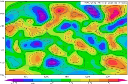
Figures 2.1, 2.2 and 2.3 show a visualization of a portion of the information available on the database demonstrated in the form of three plots containing the mean global values of temper-ature, uwind and vvind for the year of 2016 at 200 mb pressure altitude or at approximately FL390.

Figure 2.1: Temperature at 200 mb pressure level, approximately at FL 390.

Flight phase explanation Chapter 2 • Models and Algorithms

Figure 2.3: Vwind at 200 mb pressure level, approximately at FL 390.

2.2

Flight phase explanation

There are several accepted terms for each flight phase, that depend on their use as well as the organization that defined them. The flight phase terminology and definition used for the TP tool were adapted from IATA’s (International Air Transport Association) taxonomy, ICAO’s (International Civil Aviation Organization) Accident/Incident Data Reporting (ADREP) system [34] as well as Eurocontrol’s flight phase definition as used on their aircraft performance database [11]. The adapted Eurocontrol’s base of aircraft data (BADA) flight phases as defined in [35] were also used.

Each different flight phase requires several parameters for an accurate simulation such as target speed, target altitude or climb/descent rates. These values will always be respected unless it is not possible to do so. All climb and descent phases have a pre-determined thrust setting that will be maintained constant unless it must be altered in order to, for example, respect speed constraints, target altitudes or rates of climb/descent. The used terminology for each flight phase is the following:

1. Takeoff: This phase combines both the takeoff roll as well as the rotation and the takeoff phases. This phase’s thrust setting is constant at the maximum value. The parameters this phase requires are rotation speed and initial obstacle altitude. The phase ends when the initial obstacle altitude is reached.

2. Initial Climb: During the initial climb the thrust setting is set to be slightly less than the maximum value in order to minimize the increased stress the engines are subject to at maximum power setting. This phase is the steepest of all climb phases and lasts until its target altitude is reached. It requires initial climb target speed, altitude and rate of climb.

3. On Course Climb: The on course (or en route) climb starts when the aircraft has reached a high enough altitude to safely proceed ”on course” to its target destination. It requires on course climb target speed, altitude and rate of climb.

Chapter 2 • Models and Algorithms Flight phase explanation

4. Secondary Climb: The secondary climb is a continuation of the en course climb, that is usually slightly less steep. It requires secondary climb target speed, altitude and rate of climb.

5. Mach Climb: The mach climb (also called cruise climb) is the final climb phase before reaching cruise altitude, and its generally the smoothest of all climb phases. Usually most altitude related airspeed restrictions no longer apply at this altitude so the aircraft will accelerate to high speeds, close to cruising speed. As the altitude increases it is necessary to gradually reduce the flight path angle in order to ensure a close to constant speed. This phase requires mach climb target Mach number, altitude and rate of climb.

6. Cruise: During cruise the aircraft is leveled off and unlike the previous phases its power setting is adjusted to maintain the cruise phase desired speed. The cruise phase ends when the aircraft is close enough to the airport as to ensure a smooth descent. This phase requires target Mach number and distance from airport to initiate descent.

7. Initial Descent: At the start of the initial descent the power setting will be set to idle and a descending flight path is taken. This phase is usually flown at high, close to cruise, speeds. It requires target Mach number, altitude and rate of descent.

8. Main Descent: During this phase it is sometimes required for the aircraft to level off to slow down to its target speed. Once a certain altitude has been reached it is safe to extend flaps, which are crucial to reach safe approach and landing speeds. This phase requires target speed, altitude and rate of descent.

9. Approach Descent: The final descent phase is also set to be flown at idle power, however it is often required to slightly increase power for approach maneuvers. During this phase it is essential to reduce the aircraft’s speed to a safe speed for landing. This phase requires approach descent target speed.

10. Landing: During landing the aircraft is leveled off and its thrust is set to reverse mode. The simulation ends when, during this phase, the aircraft’s speed reaches zero.

Image 2.4 was retrieved from Eurocontrol’s aircraft performance database and contains the average flight phase parameters for the Boeing 777-200.

Aircraft information Chapter 2 • Models and Algorithms

2.3

Aircraft information

The aircraft information employed is divided in two main areas: aircraft parameters and aircraft flight plan typical values. The aircraft parameters were mostly retrieved from the book Civil Jet Aircraft Design data sets that contains accurate information regarding the majority of large civil transport aircraft in use today [9]. The aircraft typical flight plan values were retrieved from Eurocontrol’s Aircraft Performance database [11]. Using these sources a database of several aircraft was created and included on the TP tool, allowing the user to easily simulate several civil transport aircraft in use today. In order to contain this information the JSON (JavaScript Object Notation) file format was chosen due to its lightweight and simplicity of use, as well as its capabilities of being both easily readable and writable for humans and efficient for machines to parse and generate. The tool also allows the user to create a new aircraft entry based on existing entries or to create a completely new entry using only the GUI. Table 2.2 contains the required parameters for each aircraft.

Table 2.2: Required aircraft parameters for simulation.

Parameter name Parameter type

Maximum take-off weight [kg] Weights

Fuel Weight [kg] Weights

Number of engines Engines

Maximum sea level thrust [N] Engines Take-off engine specific fuel consumption [kg/s/N] Engines Cruising engine specific fuel consumption [kg/s/N] Engines Engine idle thrust percentage Engines

Wing span [m] Dimensions

Wing surface area [m2_{] Dimensions}

Flap to wing span ratio Dimensions Takeoff lift coefficient Aerodynamic Maximum lift coefficient Aerodynamic Parasitic drag coefficient Aerodynamic Never exceed speed (VNE) [m/s] Safety

Maximum flight path angle [o_{] Safety}

The safety parameters of never exceed speed and maximum flight path angle are to be used as limits not to be exceeded during simulation. The way they are employed on the algorithm will be explained on the next section. Some of the parameters on table 2.3 are dependent on the actual flight requirements, therefore they should be treated as an average rather than a fixed value and should be adjusted, if needed, for each flight.

Chapter 2 • Models and Algorithms Airport database

Table 2.3: Required flight parameters for simulation. Takeoff speed [m/s] Cruise altitude [m] Initial climb speed [m/s] Cruise target Mach number Initial climb target altitude [m/s] Initial descent target Mach number

Secondary climb speed [m/s] Initial descent target altitude [m] Secondary climb target altitude [m] Main descent speed [m/s]

On course climb speed [m/s] Main descent target altitude [m] On course climb target altitude [m] Approach descent speed [m/s]

Mach climb target Mach number Touch down speed [m/s]

2.4

Airport database

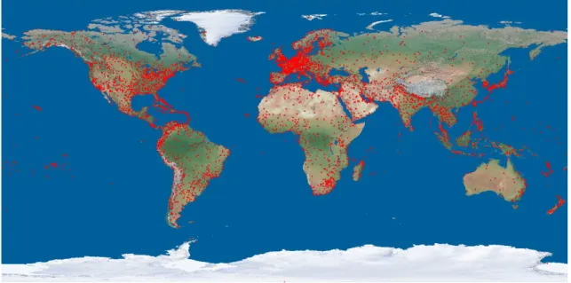
An airport and aerodrome database was incorporated into the TP tool in order to allow the user to simulate a quick trajectory without predetermined waypoints between two known airports or aerodromes. The database chosen was Openflights Airport database that contains several thousand of the world’s airports and aerodromes. This data was available in a generic informa-tion file. The used informainforma-tion for each airport entry was the airports name, IATA/ICAO code, latitude, longitude and altitude [36]. Below is an image taken directly from the TP tool showing all airport entries as red dots.

Figure 2.5: Airport database entries location.

2.5

Waypoint determination

The TP tool allows the user to simulate flight solely between a starting and a finishing waypoint and also to simulate a trajectory between a larger number of given waypoints, while calcu-lating intermediate waypoints between them as needed, in order to approach the path to a orthodromic trajectory between intermediate waypoints.

Waypoint determination Chapter 2 • Models and Algorithms

In order to approximate the trajectory between two given points to a orthodromic one, inter-mediate waypoints are calculated on a great circle (or orthodrome) between those two points. The amount of waypoints calculated depends on the position of the two original waypoints. The algorithm below calculates the latitude and longitude of a point between the two given points that is at a fraction of the total distance between them on the same orthodrome. The only requirement is that the initial points are not antipodal, as that would cause the route to be undefined. In the algorithm below f is the fraction of the distance between the given points, d is the distance in degrees between the given points, λxand φxare the latitude and longitude of

the given points and finally λf and φfare the coordinates of the calculated intermediate points

[37]. 1. A: A = sin(d(1− f)) sin(d) (2.1) 2. B: B = sin(f d) sin(d) (2.2) 3. x:

x = Acos(λ1)cos(φ1) + Bcos(λ2)cos(φ2) (2.3) 4. y:

y = Acos(λ1)sin(φ1) + Bcos(λ2)sin(φ2) (2.4) 5. z:

z = Asin(λ1) (2.5)

6. Intermediate point latitude, λf:

λf = atan2(z,

√

x2_{+ y}2_{) (2.6)}

7. Intermediate point longitude, φf:

φf = atan2(y, x) (2.7)

The angular distance d, between the given points is calculated in the following way based on the spherical law of cosines [38] where the point P is the elevated pole and A and B are the given points as illustrated in figure 2.6:

Chapter 2 • Models and Algorithms Waypoint determination

Figure 2.6: Scheme of the globe showing the points A and B on the same orthodrome, as well as the elevated pole P.

1. AB longitude variation, ∆φ:

∆φ = φ2− φ1 (2.8)

2. Angular distance between A and P, PA1_:

P A = 90± λ1 (2.9)

3. Angular distance between B and P, PB1_:

P B = 90± λ2 (2.10)

4. Angular distance between A and B, d:

d = acos(cos(∆φ)sin(P A)sin(P B) + cos(P B)cos(P A)) (2.11)

In order to determine when a intermediate waypoint is needed an iterative process determines the fraction between the initial point and the final point by calculating the Givry correction between the initial point and the would be intermediate point and comparing it to a maximum value, whose default is set to 10o_{. If the Givry correction is larger than the maximum value}

1

When calculating the angular distance of A and B from the elevated pole P (PA and PB), the mathe-matical operator depends on which elevated pole is selected (North or South) and on what hemisphere the points A and B are on. If the selected pole and the point’s hemisphere is the same the operator is positive, otherwise its negative.

Main algorithm Chapter 2 • Models and Algorithms

that intermediate waypoint is integrated in the trajectory path. In order to calculate the Givry correction (γG) between two waypoints only their coordinates are required, as can be seen

below where A and B are the waypoints used:

γG=

∆λAB

2 senφm (2.12)

The medium latitude between points A and B (φm) is given by:

φm=

1

2(φA+ φB) (2.13)

An example of the use of intermediate waypoints between given waypoints can be seen on figure 2.7, where the given waypoints are purple and the calculated intermediate waypoints are white.

Figure 2.7: An example of calculated and given waypoints retrieved from the TP tool.

2.6

Main algorithm

In this section the main algorithm’s loop will be explained step by step. Before the initiation of the loop a verification of the user input is applied, to make sure its valid. The required parameters are the aircraft characteristics described above, as well as the flight path waypoints or, at least, the initial and final waypoints. The month and time of day of the simulation, as well as attrition coefficients for the takeoff and landing phases should also be provided.

2.6.1

Time Step Calculation

Given the nature of commercial aircraft flights a variable time step (t) is valuable for their efficient (fast) simulation. This is due to the long duration of the cruise flight phase when maneuvers are limited and overall speed varies only slightly. Taking this fact into account a variable time step is used whose value depends mostly on the current flight phase and the distance to the target waypoint, diminishing the closest the aircraft is to the waypoint. Smaller

Chapter 2 • Models and Algorithms Main algorithm

values of time step are especially important during ground phases for accurate calculation of landing and takeoff distances.

2.6.2

Update climate state

When the aircraft crosses the spatial grid of the weather database new values must be retrieved from it. This is done by checking the aircraft’s current position and comparing it to its last position. Even if new database entries are not required, the weather database parameters are interpolated between entries to improve accuracy and to avoid sudden steep leaps in values.

2.6.3

Available Thrust

In this step, the maximum available thrust is calculated (at full throttle) for the current simula-tion state. As stated before, these simulasimula-tions are based on high bypass ratio turbofan engines, since these are the most widely used for large civil transportation aircraft. These engine’s thrust varies significantly with speed and altitude. Although it varies with every engine, it can be estimated by the equation below, where M is the Mach number, T0is the maximum available thrust at sea level and ρ(h) and ρ0 is the air density at the current altitude and at sea level, respectively. When M < 0.1, M = 0.1 should be used.

TA= 0.1 MT0 ρ(h) ρ0 (2.14)

2.6.4

Drag

The current total drag is calculated in this step, by combining the parasitic and lift induced drag. This tool only takes into account subsonic drag since its focus is to simulate large transport aircraft whose highest Mach numbers during cruise are usually between 0.79 and 0.86. The parasitic and induced drags are calculated below where V is the current speed, W is the aircraft weight, S is the wing surface area, CD0 is the parasitic drag coefficient and γ is the aircraft’s flight path angle.

1. Parasitic Drag (D0): D0= 1 2ρV 2_SC D0 (2.15) 2. Induced Drag (Di): Di = KW2_cos2_γ 1 2ρV2S (2.16) 3. Total Drag (D): D = D0+ Di (2.17)

The parameter K is the induced drag coefficient and can be calculated with the equation bellow where AR is the wing aspect ratio, e is the Oswald efficiency number and Kprofileis the airfoil’s induced drag factor.

K = 1

Main algorithm Chapter 2 • Models and Algorithms

2.6.5

Current Thrust and Power Setting

The way thrust and power setting is calculated in this simulation depends on the current flight phase. In phases where the power setting is constant the current thrust is simply calculated with that power setting value (δ) and the available thrust (TA). The power setting values range from 0 (zero thrust) to 1 (maximum thrust), although during flight the minimum power setting acceptable is the idle power setting, whose default value is set to be 0.1, but may be changed by the user. The default thrust setting values used are ICAO’s standard values in the Landing and Takeoff (LTO) cycle, which were defined for aircraft emission testing [39], and are shown below. These values however, are only a general approximation and sometimes differ significantly from the actual used values, which results in some intent prediction errors [40].

T = δTA (2.19)

• Takeoff: During takeoff the power setting is constant and set to the maximum value. • Climb Phases: During climb the default power setting is set to slightly less than maximum

value, at 0.85. It remains at this value unless more thrust is required to reach the current phase’s target altitude.

• Cruise: Unlike the previous phases the power setting during this phase is not constant or predetermined. During the beginning of cruise the thrust setting is kept at the previous phase’s setting while accelerating to the cruise phase target Mach number. Once the cruise target Mach number is reached the current thrust is set to be equal to the required thrust to maintain the current Mach number, and is updated every iteration, causing a changing power setting. In other words the required thrust is approximately equal to the previously calculated drag, in order to maintain a constant Mach number as the speed of sound varies only slightly on constant altitude.

• Descent Phases: During the descent phases the power setting is set to idle, except when the current aircraft speed is less than the phases target speed or the aircraft’s stall speed. In this case the current thrust is set to the required thrust to maintain constant speed, much like during the cruise phase, except in this phase the weight component must be taken into account.

• Landing: During the landing phase the thrust is set to reversed mode, with an arbitrary value of percentage of available thrust that is user dependent.

2.6.6

Flight Path

The first step to calculate the flight path angle is calculating the desired flight path, called the reference flight path (γref). This angle is calculated based on the excess thrust which is the

difference between the current thrust and the thrust required to maintain this phase’s target speed. γref = asin ( T− Trequired W ) (2.20)