Latent growth mixture modeling: an application in the aeronautic training environment

Departamento de Métodos Quantitativos

LATENT GROWTH MIXTURE MODELING:

AN APPLICATION IN THE AERONAUTIC TRAINING

ENVIRONMENT

Ana Patrícia Correia Gomes

Thesis submitted as partial requirement for the conferral of Master in Data Mining and Data Analysis

Supervisor:

Prof. Doutor José Gonçalves Dias

Setembro 2009 2 cm

Departamento de Métodos Quantitativos

LATENT GROWTH MIXTURE MODELING:

AN APPLICATION IN THE AERONAUTIC TRAINING

ENVIRONMENT

Ana Patrícia Correia Gomes

Thesis submitted as partial requirement for the conferral of Master in Data Mining and Data Analysis

Supervisor:

Prof. Doutor José Gonçalves Dias

RESUMO

A aplicação de modelo de mistura com crescimento latente a dados longitudinais oferece uma generalização importante dos modelos de crescimento convencionais, permitindo a identificação de diferentes padrões de crescimento, tendo em conta a heterogeneidade da população.

O principal objectivo deste estudo consiste em analisar o processo de aprendizagem no treino de pilotos (modelos com crescimento latente), identificar diferentes padrões de crescimento resultantes da heterogeneidade existente (modelo de mistura com crescimento latente), e identificar as variáveis explicativas da variabilidade e do padrão de crescimento. O objecto de estudo é o desempenho no treino de pilotos ab-initio (n=297), candidatos à Academia da Força Aérea Portuguesa (avaliados em seis medidas repetidas).

Os resultados obtidos demonstram que existe heterogeneidade não observada na população e que o modelo mais adequado é um modelo de mistura com crescimento latente de duas classes.

A coordenação motora (SMA) demonstrou um efeito significativo no intercepto (estado inicial) e o prognóstico de Adaptabilidade Geral (dimensão Personalidade/Motivacional) demonstrou um efeito significativo quer no intercepto (estado inicial) quer no declive (aprendizagem). A classe latente 1 (66% da amostra) caracteriza-se por apresentar uma performance em voo superior no estado inicial (intercepto), um efeito significativo da Adaptabilidade Geral no intercepto, e melhores resultados nos testes realizados na fase de avaliação psicológica. Por sua vez, a classe latente 2 (34% da amostra) apresenta piores resultados relativos ao estado inicial da performance em voo, e um efeito significativo da Adaptabilidade Geral na aprendizagem (declive).

Palavras-chave: modelos com mudança latente, modelo de mistura com crescimento latente,

treino aeronáutico, heterogeneidade não observada.

ABSTRACT

The application of growth mixture modeling to longitudinal data offers an important extension of conventional modeling tools, enabling the identification of different patterns in growth, by accounting for population heterogeneity.

The main goal of this study is to analyze the shape of the learning process in pilot training (Latent Growth Modeling), as well as to recognize different patterns in growth due to population heterogeneity (Growth Mixture Modeling). Moreover, the research intends to identify predictors that explain that variability and the pattern of growth. The object of study is the performance in flight training of ab-initio pilot applicants (n=297) to the Portuguese Air Force Academy (evaluated through six repeated measures).

The results showed the existence of unobserved heterogeneity in the population and the best fitting model is a 2-class mixture model.

Psychomotor coordination (SMA) showed a significant effect on the intercept (initial status) and the prognostic of General Adaptability (Personality and Motivation dimension) depicted a significant effect on the intercept (initial status) and on slope (development). The latent class 1 (66% of the sample) presents the highest initial flight performance, a positive significant effect of the General Adaptation on the intercept and the best results in the tests performed in the psychological phase. The latent class 2 (34% of the sample) presents the worst initial flight performance, and a positive significant effect of General Adaptation on the slope.

Keywords: latent change models, growth mixture modeling, aeronautic training, unobserved

heterogeneity.

SUMÁRIO EXECUTIVO

Os modelos com crescimento latente (MCL) apresentam-se como uma valiosa ferramenta para modelar dados longitudinais. Nos últimos anos verificou-se um interesse crescente pela utilização desta técnica, devido em parte à sua grande aplicabilidade às ciências económicas, ciências psicológicas e ao marketing.

Os modelos com crescimento latente (MCL) focam-se essencialmente na modelação de curvas de crescimento, modelando simultaneamente diferenças intraindividuais (um indivíduo ao longo do tempo) e inter-individuais (diferença entre as curvas para os vários indivíduos). É ainda assumido que a amostra provém de uma única população homogénea. Contudo, o pressuposto de homogeneidade nos parâmetros de mudança nem sempre é válido.

O modelo de mistura com crescimento latente (MMCL) é apresentado como uma extensão ao MCL, permitindo uma estrutura de clusters na modelação. Este tipo de modelos é considerado como uma segunda geração de modelos de equações estruturais com variáveis latentes, ao permitir além de variáveis latentes contínuas, também variáveis latentes discretas que definem uma tipologia de grupos e permite modelar populações heterogéneas.

Este trabalho foi aplicado ao meio aeronáutico, nomeadamente ao processo de aprendizagem no treino de pilotos militares, tendo como principal objectivo identificar diferentes padrões de crescimento resultantes da heterogeneidade existente, e variáveis explicativas da variabilidade e do padrão de crescimento. O objecto de estudo é o desempenho no treino de pilotos ab-initio (n = 297), candidatos à Academia da Força Aérea Portuguesa (avaliados em seis medidas repetidas). A amostra é constituída pela totalidade de candidatos, que entre os anos de 2001 a 2008 completaram com sucesso as provas psicológicas, médicas e físicas. As seis medidas repetidas são operacionalizadas pelos desempenhos obtidos nos seis voos do Estágio de Selecção de Voo (ESV). O Estágio de Selecção de Voo constitui a última etapa do processo de selecção e tem como principal objectivo a eliminação dos candidatos que não se consigam adaptar às exigências do meio aeronáutico. São também incluídas neste estudo, variáveis preditoras do cluster e do crescimento latente, nomeadamente a coordenação motora, a aptidão espacial e o prognóstico de adaptabilidade.

Os resultados obtidos demonstram que existe heterogeneidade não observada na população e que o modelo mais adequado é um modelo de mistura com duas classes. A coordenação

demonstrou um efeito significativo quer estado inicial quer na aprendizagem. A classe latente 1 (66% da amostra) caracteriza-se por apresentar uma performance em voo superior no estado inicial e um efeito significativo do prognóstico de adaptabilidade no estado inicial. Por sua vez, a classe latente 2 (34% da amostra) apresenta piores resultados relativos ao estado inicial da performance em voo, e um efeito significativo do prognóstico de adaptabilidade na aprendizagem.

O MMCL com variáveis ordinais está ainda em desenvolvimento e encontram-se ainda muito poucos trabalhos publicados com aplicações, e mesmo os próprios pacotes estatísticos estão ainda em fase de aperfeiçoamento. O presente trabalho apresenta-se como um contributo para a exploração desta abordagem como também uma primeira tentativa de modelação longitudinal da performance aeronáutica.

ACKNOWLEDGMENTS

I would like to thank some people, who directly or not contributed to the completion of this master´s thesis:

First, I wish to thank my supervisor, Professor José Gonçalves Dias, about the way he supervised me through this study. His endless enthusiasm, dedication and guidance have encouraged me to bring this research into completion. I am deeply indebted to him for his help.

I would like to thank to the Portuguese Air Force Psychology Center for giving me the opportunity of developing this research, and to all pilot applicants that made this work possible.

Special thanks to my dear friends for their support and encouragement.

I would also like to express thanks to my family for their love and understanding.

I also wish to thank my fiancé’s family for their friendship.

Finally, I would like to thank my fiancé Tó, for the unconditional support throughout this process, companionship, concern, and helpful advices in the decisive moments, which made it possible to achieve this goal.

INDEX

2 LATENT GROWTH MIXTURE MODELING... 5

2.1 INTRODUCTION ... 5

2.2 LATENT GROWTH CURVE MODELS ... 6

2.2.1 Model Specification ... 6

2.2.2 Model Estimation ... 8

2.2.3 LGM with Covariates ... 9

2.2.4 Measurement Model for Ordinal Variables ... 9

2.3 LATENT GROWTH MIXTURE MODELING ... 11

2.3.1 Background ... 11

2.3.2 Model Specification ... 13

2.3.3 Model Estimation ... 16

2.4 MODEL ASSESSMENT ... 17

2.4.1 Akaike information criterion (AIC) ... 18

2.4.2 Bayesian Information Criterion (BIC) ... 18

2.4.3 Adjusted Bayesian Information Criterion (aBIC) ... 18

2.4.4 Lo-Mendell-Rubin likelihood ratio test – LMR LRT ... 19

2.5 SYNTHETIC DATA EXAMPLE ... 20

3 EMPIRICAL STUDY ... 23 3.1 INTRODUCTION ... 23 3.2 HYPOTHESES ... 24 3.3 DATA ... 25 3.3.1 Sample ... 25 3.3.2 Flight Screening (FS) ... 25 3.3.3 Covariates ... 29

3.3.3.1 Personality and Motivation Dimension ... 29

3.3.3.2 Perceptive-cognitive and Psychomotor Dimension ... 31

3.4 EMPIRICAL RESULTS ... 34

3.4.1 Single-class growth curve model – Assuming homogeneity ... 34

3.4.2 Checking population heterogeneity ... 36

3.4.3 Selecting the appropriate number of latent classes ... 37

3.4.4 Two-class Mixture Model ... 39

3.4.5 LGMM with Covariates ... 43

4.1 EMPIRICAL FINDINGS ... 51

4.2 LIMITATIONS AND RECOMMENDATIONS FOR FURTHER RESEARCH ... 52

REFERENCES ... 55

ACRONYMOUS

ABIC Adjusted Bayesian Information Criterion

AIC Akaike Information Criterion

ANCOVA Analysis of Covariance

ANOVA Analysis of Variance

BIC Bayesian Information Criterion

CAIC Consistent Akaike Information Criterion

CFI Comparative Fit Index

EM Expectation Maximization

FS Flight Screening

GGMM General Growth Mixture Model

GMM Growth Mixture Modeling HLM Hierarchical Linear Modeling

INS2 Instruments 2

LCA Latent Class Analysis

LCM Latent Curve Model

LGM Latent Growth Model

LGCM Latent Growth Curve Model

LMR – LRT Lo-Mendell-Rubin likelihood ratio test MANOVA Multivariate Analysis of Variance

ML Maximum Likelihood

NNFI Non-Normed Fit Index

PILAV Pilot Aviator

PoAFA Portuguese Air Force Academy

RMSEA Root Mean Square Error of Approximation

SEM Structural Equation Model

SMA Sensory Motor Apparatus

LIST OF FIGURES

Figure 1 – Representation of the growth mixture model. ... 14

Figure 2 – Representation of the model being simulated. ... 20

Figure 3 – Scores obtained in the selection flights. ... 26

Figure 4 – Recoded scores obtained in the selection flights... 27

Figure 5 – Hands (spatial aptitude test). ... 32

Figure 6 – Instruments interpretation. ... 32

Figure 7 – Sensory Motor Apparatus. ... 33

Figure 8 – Representation of the single class mixture model. ... 35

Figure 9 – Growth curve for a single latent class model. ... 35

Figure 10 – Model assessment. ... 38

Figure 11 – Two-class mixture model... 40

Figure 12 – Growth curve for each of the two latent class membership. ... 41

Figure 13 – Two-class mixture model with covariates. ... 43

LIST OF TABLES

Table 1 – Parameter estimates for latent class 1 (simulated data set). ... 21

Table 2 – Parameter estimates for latent class 2 (simulated data set). ... 22

Table 3 – Applicants per year and results of the FS. ... 26

Table 4 – Flight scores frequencies. ... 27

Table 5 – Recoded flight scores frequencies. ... 28

Table 6 – Summary of categorical data proportions. ... 28

Table 7 – Personality and Motivation Dimensions. ... 30

Table 8 – Descriptive statistics for General Adaptability. ... 31

Table 9 – Descriptive statistics. ... 34

Table 10 – Parameter estimates – single latent class. ... 36

Table 11 – Vuong-Lo-Mendell-Rubin likelihood ratio test for 1 (H0) versus 2 classes ... 37

Table 12 – Lo-Mendell-Rubin Adjusted LRT test. ... 37

Table 13 – Model selection criteria. ... 38

Table 14 – Vuong-Lo-Mendell-Rubin likelihood ratio test for 2 (H0) versus 3 classes ... 39

Table 15 – Lo-Mendell-Rubin Adjusted LRT test (2 versus 3 classes) ... 39

Table 16 – Final latent class proportions and classification. ... 41

Table 17 – Parameter estimates (unconditional model). ... 42

Table 18 – Final latent class proportions and classification (conditional model). ... 44

Table 19 – Parameter estimates for latent class 1 (conditional model). ... 44

Table 20 – Parameter estimates for latent class 2 (conditional model). ... 45

Table 21 – Parameter estimates (conditional model). ... 46

1 Introduction

Recent developments in latent growth modeling (LGM) provide a better tool to model longitudinal data than traditional statistic methods. Longitudinal modeling is frequently encountered in behavioral research (Muthén and Curran, 1997). No matter the subject area or the time interval, social and behavioral scientists have a strong interest in describing and explaining the time trajectories of their variables (Bollen and Curran, 2006). Latent growth modeling postulates the existence of latent trajectories. The term latent stands for a process that is not directly observed. The trajectory process is observed only indirectly using manifest repeated measures. However, this trajectory can differ at individual level (Bollen and Curran, 2006). In the recent years there has been a growing interest among researchers in the use of latent growth modeling (Jung and Wickrama, 2008). These techniques have become popular in applied social and psychological sciences, in part due to its software implementation (e.g., Mplus, Gllamm).

The statistical analysis of data over time appears in the nineteenth century. The studies were oriented taking into account the change in groups rather than in individuals. The focus on aggregate change continued in the twentieth century. These early applications utilized mostly complex functional forms of growth (e.g., nonlinear polynomials and logistic curves) to examine change in an entire group of individuals (Bollen and Curran, 2006). The theory of LGM appeared two decades ago with McArdle and Epstein (1987) and Meredith and Tisak (1990). This model estimates growth function with fixed and random parts, which describes the average development in the population as well as the variation of individual development, respectively (McArdle and Epstein, 1987; Meredith and Tisak, 1990; Willett and Sayer, 1994). These methods allow researchers to move beyond the use of ad-hoc categorization procedures for constructing developmental trajectories.

This modeling approach has been extended to include the estimation of the impact of covariates on individual growth as well as (besides observed variables with continuous scale) categorical variables (Muthén, 2004a). The estimation of model parameters can be handled using structural equation modeling (SEM) programs, such as LISREL (Jöreskog et al., 1999), EQS (Bentler, 1995), Amos (Arbuckle, 2006) and Mplus (Muthén and Muthén, 1998-2007).

In recent years, the extensiveness and intensity of longitudinal studies have raised, and a particularly attention has been given to “inter-individual variation” (variation between individuals) and “intra-individual variation” (variation within individuals). The approaches focusing on inter-individual variation point out to the establishment of general development principles that apply to all individuals. On the other hand, approaches focusing on intra-individual variation emphasize understanding change within intra-individuals, viewing the establishment of general principles as a secondary aim. Growth is a phenomenon that occurs within the individual, and therefore intra-individual variability is a primary interest in statistical modeling of longitudinal data (McGrath and Tschan, 2004).

Latent growth models can analyze the development of individuals in one or more outcome variables over time. Observed outcome variables can be continuous, censored, binary, ordered categorical (ordinal), counts, or combinations of these variable types if more than one growth process is being modeled. In a latent variable modeling framework, the random effects are conceptualized as continuous latent variables, that is, growth factors are used to capture individual differences in development (Muthén and Muthén, 1998-2007).

Another important recent latent variable modeling extension connected with the SEM context is mixture modeling. This modeling is based on the idea that population contains subpopulations, i.e. latent classes. These classes can be identified and their parameters estimated (Muthén and Shedden, 1999; Muthén, 2001). The distribution of observed variables is over a mixture distribution, so that each subpopulation has its own model parameters values (Lubke and Muthén, 2005).

Different terminologies are used in this context. For example, Muthén (2004a) uses the term “latent growth curve model”, whereas Meredith and Tisak (1990) uses the term “latent curve analysis” to refer the modeling of growth in the context of SEM. When viewed from a SEM perspective, the model is called latent growth model (Hoeksma and Kelderman, 2007). On the other hand, the term “latent growth mixture modeling” (LGMM or LGM modeling; Muthén, 2001; Muthén, 2004a), in turn, is used to refer to the combination of latent growth curve modeling and mixture modeling.

Despite twenty years old, the LGM and LGMM are novel methods in practice. As these methodologies become more common and important to model development, the functionality of the models needs more research. Because most of inferential analysis is based on asymptotic results, researchers can trust the results when sample size is large, at least 1000 observations. However, in many empirical studies, sample size is limited, say, to 100-500 observations. With simulated data is possible to examine the performance of these methods with different sample sizes (Bauer and Curran, 2003; Muthén, 2004a).

The main goal of this thesis consists in modeling and understanding the nature and heterogeneity in pilot performance development. This study focuses on two different types of data: simulated data sets (n=500, n=1000, n=5000, n=10000), and an empirical example (n=297) from the aeronautic training context. The simulated data makes it possible to draw conclusions concerning the performance of LGMM with different sample sizes, while the application of LGMM in empirical data shows that this approach is able to capture the underlying process being modeled. Methods for latent growth modeling do allow incorporating attributes that can help improve predictions and, hence, design more effective interventions. Indeed, at the moment the performance in flight has been studied in the perspective of trying to find predictors of flight performance (Burke and Hunter, 1995). However, the dichotomous split of training success into pass versus fail dominates the pilot selection literature (Roe, 2008).

Martinussen (2003) pointed out that the supported interest in the theme of pilot selection drifts essentially of the high cost associated to pilot training mainly due to the use of aircrafts. The search for better predictors of success in pilot training is connected to high costs related to personnel training, and the need for recruiting competent and well-suited people. According to the same author, the cognitive and the psychomotor measures were pointed out as the best predictors of flight performance.

Previous studies concerning pilot performance in PoAF (Portuguese Air Force) identified key aptitudes as predictors of flight performance (Bártolo-Ribeiro et al., 2004). The tests applied in the psychological phase, concerning the assessment of the psychomotor coordination (Sensory Motor Apparatus - SMA) and spatial aptitude (INSB2 and Hands) are predictors of pilot training successful performance. This fact is not surprising as the spatial aptitude and motor coordination are two factors strongly related to the flight adaptation.

Concerning the training of military pilots, the candidates have little or even no experience in the field of the aviation. After initial screening (psychological, medical and physical phases), the pilot candidates accomplish a selection training program, the FS (Flight Screening), composed by seven flights, in which they have to demonstrate their learning capabilities. This research analyzes the shape of the learning process in pilot training (LGM), allowing for heterogeneous patterns of growth due to sample heterogeneity (GMM).

Next, we present the structure of this thesis. Chapter 2 gives an overview of LGM and LGMM frameworks. Section 2.1 consists of an introduction to the setting of LGM. In Section 2.2, the LGM is discussed in four stages: model specification, inclusion of covariates, model estimation, and the application to ordinal variables. The LGMM framework is explored in Section 2.3, and Section 2.4 discusses model assessment. Section 2.5 illustrates these approaches using simulated data sets. Chapter 3 deals with the empirical application. Section 3.1 gives an overview to the pilot evaluation framework, Section 3.2 presents the study hypotheses, Section 3.3 describes the data set, Section 3.4 provides the results and Section 3.5 provides a discussion of the empirical results. The thesis ends with a final chapter in which a summary of main conclusions, major limitations of this research, and suggestions for further research are provided.

2 Latent Growth Mixture Modeling

2.1 Introduction

The most applied approach to modeling change with continuous variables is growth curve models. They fit growth trajectories for individuals and relate characteristics of these individual growth trajectories (e.g., slope) to covariates (Collins, 2005).

One type of analytic technique designed to address questions of individual differences in change over time is referred to as random coefficients modeling. The translation into latent variable models can be made using a simple random coefficient growth curve model as a starting point that illustrates the key features of the latent variable longitudinal model approach (Curran and Muthén, 1999).

The latent growth model (LGM) is commonly composed of two factors. The first and second factors relate to the level (i.e., intercept) and slope of growth, respectively. These two factors correspond to the mean value of the intercept and slope and individual random variation of these two latent components. Slope is either fixed to describe linear change or, alternatively, the pattern of slope is estimated (Aunola et al., 2004).

2.2.1 Model Specification

In LGM the focus of interest is on the average development over time and individual variation around this average. The pattern of slope component is the same for each individual, but the strength of this pattern may vary individually (Collins, 2005). It is possible to define the latent growth model in two parts:

a) Measurement Model

and = 1,2,…T, (1)

where

is the observation of individual i at the time point t, is the intercept component of individual i,

is the linear slope component for individual i,

is the measurement error for individual i at the time point t, n is the number of observations and

T is the number of time points.

The intercept and slope parameters are random effects; in other words, they may vary across individuals, as reflected in the need for the subscript denoting individual.

b) Latent Model

(2)

where and are expected values (fixed part of the model) of latent growth factors and , respectively; and and are random variables that configure individual growth. This model describes linear growth over time, so that intercept ( ) and slope ( ) represent

the initial status and linear growth rate of the growth trajectory of individual i, respectively (Curran and Muthén, 1999).

The standard latent curve can be presented by using a general SEM framework (Hipp and Bauer, 2006)

+

(3)

where is a vector of observed repeated measures for individual i, where T is the number of waves of data, is a vector of latent growth factors (or random coefficients; i.e., intercept and slope), is a a vector of measurement errors, and is a 2 1 vector of expected values of .

We assume further that = 0 and = 0, and

COV ( )

COV = ,

(4)

where is the T covariance matrix of the time-specific residuals and is the 2 covariance matrix of the growth factors.

The mean vector and covariance matrix of are

COV . (5)

The mean vector and the covariance matrix of the observed variables y are

,

COV = . (6)

where is the variance-covariance matrix of , and represent the covariance structure of and , respectively. The functional form of the individual trajectories is defined by fixing

before. It is traditionally assumed that the growth factors and time-specific residuals are multivariate normally distributed as

. ₍₇₎

According to equation (5), the T vector y follows the multivariate normal distribution

( i = 1,2,…n, (8)

where and are given in equation (6).

2.2.2 Model Estimation

Maximum-likelihood (ML) estimation is carried out by maximizing the log-likelihood function (Muthén and Khoo, 1998). Raykov (2005) refers that this is a very popular estimation and testing framework. Its essence is the estimation of unknown parameters that underlie an assumed model by values that maximize the probability of observing the data at hand (probability density). ML is employed for parameter estimation, model fit evaluation, and hypothesis testing purposes, in particular when examining hypotheses of parameter restrictions via likelihood-ratio tests. The application of the ML method for parameter estimation assumes here the multivariate normality of the observed data. The distribution of the observed (independent) individual is given by the product of “probabilities”. This product is viewed as dependent on the unknown characteristics of the underlying distribution, such as means, variances, and covariances.

Let be a k vector, which consists of all free parameters in . The parameters can be estimated using the maximum likelihood estimation (ML).

The likelihood function is the probability density of the observed data considered as a function of the model parameters. For a set of n independent observations (given), the likelihood function can be expressed as

, (9)

and the log-likelihood can be expressed as

. (10)

This log-likelihood function can be maximized iteratively by the Newton-Raphson algorithm.

2.2.3 LGM with Covariates

It is possible and desirable to include predictors in addition to time. Let the latent growth for a single outcome variable y observed for individual i at time point t be related to a covariate . In this case, considering only one covariate, the idea is that each individual has his or her own growth trajectory. Growth will be expressed in terms of an LGM, with the inclusion of predictors:

+ . (11)

The log-likelihood function of the conditional model turns out to be more difficult to maximized and time consuming as it demands for numerical integration.

2.2.4 Measurement Model for Ordinal Variables

Modeling ordinal variables is relatively new in the applied SEM literature.In ordinal repeated measures designs, the data consist of a multidimensional contingency table. A model for ordinal repeated measures must predict the proportion of individuals within each response pattern in terms of hypothesized model parameters. A Latent Growth Curve Model for ordinal panel data is a model of multivariate proportions. An LGC model, however, imposes restrictions on sample means and covariances rather than on sample proportions. Therefore, we must somehow extract means and covariances from the observed ordinal proportions (Mehta et al., 2004).

A growth model for ordinal measures predicts joint ordinal proportions. The LGC model hypothesizes that the observed response at each time point t is related to the

thresholds are hypothesized to relate the unobserved scores on the latent variable, with the observed ordinal responses at each time point t. The underlying latent variables ( are assumed to follow a multivariate normal distribution with unknown means and covariance. In the analysis of categorical variables, thresholds are provided for each increased scale level, or we can say that each threshold represents a portion of the underlying continuous scale. For example, the observed variable is represented by y, with three categories, and represents the underlying latent or unobserved continuous variable. An ordinal variable does not have a metric scale, so the latent response variable is used to describe the relationship between that categorical variable and other variables in the model.

The relationship between an observed ordinal measure (y), with R response categories (r = 0, ... , R - 1) and underlying continuous variable ( ), can be defined by means of R - 1 thresholds ( ) as (Mehta et al., 2004):

, (12)

where and = . If is assumed to be normally distributed the probability that is less than or equal to is:

, (13)

where Ф is the cumulative standard normal distribution and E( ) and SD( ) are the mean and standard deviation of the latent variable , respectively. Equation (13) gives the cumulative probability that the latent continuous is less than or equal to the rth threshold τr. The probability that the observed ordinal Y is equal to a given category r is:

) – P ( . (14)

The thresholds define the cutoff points on a normal distribution. For a given mean and standard deviation of and the two thresholds (τr and τr+1), the probability that y is in category r (i.e., the probability that y is between the two thresholds) is the area under the standard normal curve bounded by the two thresholds on the z scale (

The correlation between pairs of outcomes is called the polychoric correlation coefficient when ordinal variables have a bivariate normal distribution. The correlation between an ordered categorical outcome and a variable measured on a continuous interval scale is called the polyserial correlation coefficient. Correlations such as the polychoric correlation are not computed from actual observed variables but rather from theoretical correlations of the underlying variables. The use of these variables allows the focus of growth to be on changes in the continuous variables . In spite of this, the formulation can also be used to focus on changes in the probabilities of y (Duncan et al., 2006).

2.3 Latent Growth Mixture Modeling

2.3.1 Background

Growth curve models, as have been seen in the previous section, focused on growth curve modeling that considers both intra-individual change and inter-individual differences in such change, but treats observed data as if collected from a single homogeneous population. Conventional latent growth modeling can be used to estimate the amount of variation across individuals in the latent growth factors (random intercepts and slopes) as well as the average growth. In other words, in a conventional latent growth model the individual variation around the estimated average trajectory is expressed as growth factors that are allowed to vary across individuals (Kreuter and Muthén, 2008). This assumption of homogeneity in the growth parameters does not always correspond to the reality, and if heterogeneity is ignored, statistical analyses and their effects can be seriously biased.

Latent growth mixture modeling assumes that the population of interest is not homogeneous (as measured by response probabilities) but consists of heterogeneous subpopulations with varying parameters, allowing for within-class variation (Muthén, 2006). The common theme in mixture modeling is the partition of the population into an unknown number of latent classes or subpopulations (Duncan et al., 2002).

Mixture analysis also known as latent class analysis (LCA) describes how the probabilities of a set of observed categorical variables or indicators vary across groups of individuals, where group membership is not observed. For example, the observed categorical variables may

unobserved groups of individuals as latent classes. LCA attempts to find the smallest number of latent classes that can describe the associations between the observed categorical variables. The analysis adds classes until the model fits the data well. The parameters of the model are the probabilities of being in each class and the probabilities of fulfilling each criterion given class membership. In addition, the latent class model provides estimates of class probabilities for each individual. These values are called posterior probabilities. LCA may relate the probability of class membership to a set of background variables.

The main objective of latent class analysis is: 1) to estimate the number and size of the latent classes in the mixture; 2) to estimate the response probabilities for each indicator given the latent class; 3) to examine the fit of the model to the data using various test statistics, and 4) to assign individuals to each latent class (Duncan et al., 2002).

Muthén (2003) explored new ways of constructing more complex models that are better suited and more flexible to assessing change than conventional latent growth modeling. Muthén proposed an extension of current LGM methodology that includes relatively unexplored mixture models, such as growth mixture models, mixture structural equations, and models that combine latent class analysis and structural equation modeling (Muthén and Shedden, 1999, Duncan et al., 2002; Muthén et al., 2003). Muthén (2001) considers growth mixture modeling as a second generation of structural equation modeling.

The general framework proposed by Muthén and colleagues (Muthén and Shedden, 1999; Nagin, 1999; Muthén, 2001; Muthén, 2003; Muthén et al., 2002; Muthén et al., 2003) provides new opportunities for latent growth modeling. Growth mixture models (GMM) are applicable to longitudinal studies where individual growth trajectories are heterogeneous and belong to a finite number of unobserved groups. Muthén and colleagues (Muthén and Shedden, 1999; Muthén et al., 2002; Muthén, 2003; Muthén et al., 2003; Kreuter and Muthén, 2008) proposed the growth mixture modeling approach, combining categorical and continuous latent variables in the same model, in what they called a general latent growth mixture model framework (GGMM). The GGMM approach allows for unobserved heterogeneity in the sample, where different individuals can belong to different subpopulations.

Mixture modeling generally refers to modeling with categorical latent variables that represent mixtures of subpopulations in which population membership is not known a priori, but it is inferred from the data. In mixture modeling, unobserved heterogeneity in the development of a variable through time is captured by categorical and continuous latent variables. In particular, GMM relaxes the single-population assumption of conventional LGM method by allowing parameter differences across unobserved subpopulations. GMM allows within-class individual variation for the latent-growth factors that is captured by nonzero intercept and slope variances within latent classes. As in conventional LGM, the within-class individual variation is represented by random effects (i.e., continuous latent variables). Nevertheless, instead of considering individual variation around a mean growth curve, the growth-mixture model allows different classes of individuals to vary around different mean growth curves within each latent class (Wang and Bodner, 2007).

2.3.2 Model Specification

The GGMM modeling approach provides the joint estimation of: 1) a conventional finite mixture growth model where different growth trajectories can be captured by class-varying random coefficient means (the part that explains the latent classes); and 2) a logistic regression of outcome variables on the class trajectory (the conditional distribution in each latent class).

The model can be extended to estimate varying class membership probability as a function of a set of covariates (i.e., for each class the values of the latent growth parameters are allowed to be influenced by covariates) and to incorporate outcomes of the latent class variable (Duncan et al., 2002).

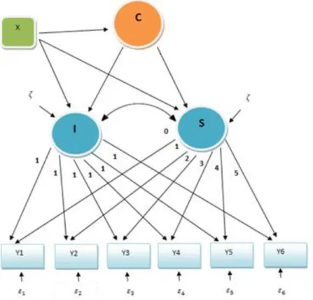
Figure 1 – Representation of the growth mixture model.

The full growth mixture model is depicted in Figure 1 (Muthén and Shedden, 1999; Muthén, 2001; Duncan et al., 2002; Muthén, 2004b). This model contains a combination of a continuous latent growth variable, (j = Intercept and Slope) and a latent categorical variable, C, with K classes, = ( , ..., ) where = 1 if individual i belongs to class k and zero otherwise. These latent variables are represented by circles in Figure 1.

In our case the continuous latent growth variable portion of the model represents conventional latent growth modeling with multiple indicators Y measured, let us say at six time points. The categorical latent variable is used to represent latent trajectory classes underlying the latent growth variable, η. Latent class and latent continuous variables can be predicted from a set of covariates (background variables), X, because the model allows the mixing proportions to depend on prior information and subject-specific variables.

In this model (Figure 1), the directional arrows from the latent trajectory classes to the growth factors indicate that the intercepts and slopes of the regressions of the growth factors on X vary across the classes of C.

Regarding the observed part of the model, multivariate normality is assumed for 1 conditional on and class k,

+ ,

and by including covariates it turns out to be

. (15)

The model relates C to , by multinomial logistic regression for K classes (Muthén, 2004b):

, (16)

where V is the number of covariates. The multinomial logistic model is identified with null coefficients for class K, i.e., 0 v = 0,…,V.

The implied structure for a six-wave model is

= .

The mean vector of (without covariates) is expressed as

(17)

The covariances matrices of _{N (0,} ) and _{N (0,} ) both assumed to be uncorrelated with other variables, and with each other, are

1

COV .

(18)

Muthén and Shedden (1999) states that the model identification implies some parameter restrictions which have to be determined, as not all parameters can be estimated uniquely.

2.3.3 Model Estimation

Parameters are estimated by Maximum Likelihood (ML), using the Expectation- Maximization (EM) algorithm. The estimation of LGMM consists of two parts: the estimation of parameters related to the LGM and the estimation of class proportion (Yung, 1997; Muthén and Shedden, 1999; Dias, 2004). The log-likelihood function of observed data for the LGMM is

log L = ), (19)

where the density function f is mixed from K density functions

) (20)

and is the proportion of subpopulation in the population. The density function in class is

, (21)

where the observed data vectors are drawn from a multivariate normal distribution with mean vector and covariance matrix (in the case without covariates).2

Parameters are estimated using either the EM algorithm (Dempster et al., 1977; Dias, 2004) or the Newton-Raphson algorithm. Each iteration of the EM algorithm involves two steps: the

2

The default estimator for this type of analysis with ordinal variables is maximum likelihood with robust standard errors using a numerical integration algorithm. Note that numerical integration becomes increasingly more computationally demanding as the number of factors and the sample size

E–Step (Expectation Step) that estimates the conditional mean of the missing variable given the previous estimate of the model parameters and the observed data, and the M–Step (Maximization Step), that re-estimates the model parameters given the observed data and the soft clustering done by the E–Step. This algorithm is known for being a general method for ML estimation with incomplete data that reintroduces the additivity of the log-likelihood function using data augmentation (Dias, 2004).

2.4 Model Assessment

Model evaluation for latent growth mixture modeling (Duncan et al., 2002) does not differ much from conventional SEM for homogeneous populations (Muthén et al., 2002). For comparison of fit of models that have the same number of classes and are nested, the usual likelihood ratio chi-square difference test can be used. There exist a number of methods to evaluate the degree of fit of the hypothesized model to data and to assess whether the fit can be improved as a function of testing alternative models (Duncan et al., 2006). Some of the indices of fit commonly used in latent growth modeling are the chi-square test statistic, the comparative fit index (CFI), and the root mean square error of approximation (RMSEA).

Testing and evaluating the overall fit is not possible, in the context of the mixture model, as it is in the framework of conventional structural equation models. Given the problems associated with the use of the likelihood ratio test for model selection, a variety of information-based criteria have been proposed to evaluate models with different numbers of latent classes. For this purpose the following criteria, provided by the current Mplus program, are used: Akaike’s information criterion (AIC), Bayesian information criterion (BIC), and adjusted BIC (aBIC). Moreover, the Lo-Mendell-Rubin likelihood ratio test is available as well (Lo et al., 2001). Sample-size adjusted BIC (aBIC) has been shown to give superior performance in simulation studies for latent class analysis models (Muthén, 2003). The recommendation is to choose a model with the smallest AIC, BIC, or aBIC value (Li et al., 2001).

Akaike information criterion, developed by Hirotsugu Akaike under the name of "an information criterion" (AIC) in 1971 and published in Akaike (1974), is a measure of the goodness of fit of an estimated statistical model. This measure is intended for model comparison and not for the evaluation of an isolated model. AIC takes into account the statistical goodness-of-fit and the number of parameters that must be estimated to achieve that degree of fit. The model that produces the minimum AIC might be considered, in the absence of other substantive criterion, as the potentially more useful model (Duncan et al., 2006).

The Akaike Information Criterion (AIC) is defined as

AIC = , (22)

where d is the number of free parameters and is the maximized value of the likelihood function for the estimated model (Muthén, 2004a). When comparing two competitive models, the best one is the one that has the lower AIC.

2.4.2 Bayesian Information Criterion (BIC)

As an alternative to AIC one can use BIC (Nagin, 1999). For a given model, BIC (Schwarz, 1978) is calculated as follows:

BIC = + d n, (23)

where is the value of the model's maximum likelihood, n is the sample size, and d is the number of parameters in the model (Nagin, 1999).

2.4.3 Adjusted Bayesian Information Criterion (aBIC)

The adjusted BIC (Sclove, 1987) replaces the sample size n in the BIC equation (24) with (n + 2) /24, resulting in (Nylund et al., 2007):

2.4.4 Lo-Mendell-Rubin likelihood ratio test – LMR LRT

Lo et al. (2001) proposed a likelihood ratio-based method for testing K − 1 classes versus K classes. The Lo–Mendell–Rubin likelihood ratio test (LMR LRT) avoids the classical problem of chi-square testing based on likelihood ratios. This concerns models that are nested but where the more restricted model is obtained from the less-restricted model by a parameter assuming a value on the border of the admissible parameter space, in the present case a latent class probability being zero. It is known that such likelihood ratios do not follow a chi-square distribution. LMR considers the same likelihood ratio but derives its correct distribution. A low p value indicates that the (K-1) class model has to be rejected in favor of a model with at least K classes. The LMR LRT procedure was implemented in Mplus (Muthén and Muthén, 2001).

: number of classes is K-1

: number of classes is K. (25)

Lo et al. (2001) proposed that the above described Lo–Mendell–Rubin likelihood ratio test should adjust with the numbers of and of freely estimated parameters in K and K-1 classes, respectively, and sample size.

The adjusted test, called the LMR test, is then

LMR = (26)

where

VLMR = (27)

and, where f (.) and g (.) define the density function under K and K- component normal mixture density, respectively. The LMR test follows a weighted chi-squared distribution.

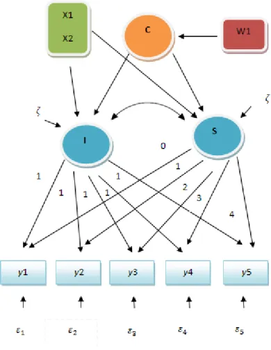
In this section the latent growth mixture model is applied to simulated data sets to demonstrate the framework delineated before. The observed data are composed by five measures, measured at five equally spaced time points (y1-y5). This latent growth model includes two latent growth factors: intercept and slope . x1 and x2 represent regression factors for intercept and slope, and w1 is a covariate. The values of x1, x2, and w1 were sampled from the standard normal: . This model was simulated in MATLAB for four data sets (n=500, n=1000, n=5000 and n=10000). The simulated data sets are estimated in Mplus (Muthén and Muthén, 1998-2007). This small simulation study illustrates the impact of sample size on parameter recovery. An LGMM is estimated for a two group solution.

The starting values of the parameter estimates were set at zero. The Mplus file used for the estimating of data set with n = 500 is given in Appendix A.1. We can see in Tables 1 and 2 the effect of sample size on parameter estimates.

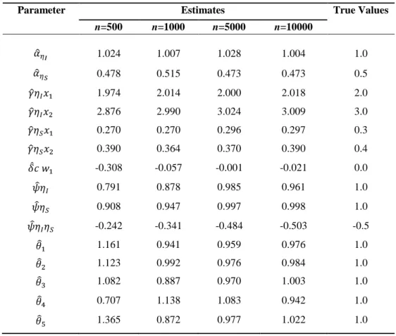
Table 1 – Parameter estimates for latent class 1 (simulated data set).

Parameter Estimates True Values

n=500 n=1000 n=5000 n=10000 1.024 1.007 1.028 1.004 1.0 0.478 0.515 0.473 0.473 0.5 1.974 2.014 2.000 2.018 2.0 2.876 2.990 3.024 3.009 3.0 0.270 0.270 0.296 0.297 0.3 0.390 0.364 0.370 0.390 0.4 -0.308 -0.057 -0.001 -0.021 0.0 0.791 0.878 0.985 0.961 1.0 0.908 0.947 0.997 0.998 1.0 -0.242 -0.341 -0.484 -0.503 -0.5 1.161 0.941 0.959 0.976 1.0 1.123 0.992 0.976 0.984 1.0 1.082 0.887 0.970 1.003 1.0 0.707 1.138 1.083 0.942 1.0 1.365 0.872 0.977 1.022 1.0

Parameter Estimates True Values n=500 n=1000 n=5000 n=10000 -1.114 -0.948 -0.956 -0.996 -1.0 -1.476 -1.610 -1.573 -1.527 -1.5 -2.224 -1.978 -2.011 -2.005 -2.0 -2.974 -2.930 -2.957 -3.005 -3.0 -0.282 -0.320 -0.284 -0.283 -0.3 -0.453 -0.347 -0.433 -0.361 -0.4 -0.308 -0.057 -0.001 -0.021 0.0 4.999 4.919 5.243 4.877 5.0 5.648 4.863 4.968 5.166 5.0 0.072 0.719 0.512 0.537 0.5 0.612 0.974 1.035 0.970 1.0 1.097 1.012 1.004 1.005 1.0 0.937 0.992 1.031 1.029 1.0 1.218 1.235 1.001 0.915 1.0 1.197 0.610 0.898 1.071 1.0

It was possible to retrieve the cluster structure (discrete latent variable) and the growth structure (continuous latent variables). As expected, increasing sample size improves the approximation to the true values.

3 Empirical Study

3.1 Introduction

The main goal of this empirical study is to analyze the shape of the learning process in pilot training and to identify the variables that can explain the pattern of growth. As not all the applicants adapt themselves to the demands of the aeronautic environment, we allow different patterns of learning, such as different levels of abilities (initial status of performance).

Psychological tests have been used in military pilot selection since the beginning of the 19th century (Martinussen, 2003). World War I, and especially World War II, were creative periods for research on both assessment program construction, personnel selection, and test and program validation. The search for better predictors of success in pilot training is probably a function of the high costs related to personnel training, human suffering from failure to complete, and the need for recruiting competent and well-suited people. Burke and Hunter (1995) divide the measures used in the pilot selection in four different categories: the cognitive measures, the personality tests, the psychomotor measures, and the measures of “job sample”. On the basis of 50 studies in the pilots selection field, the psychomotor measures were pointed out as the best predictors of the performance in flight. In a recent study, Kokorian (2008) looked at levels of prediction of simulator performance where simulators are used as one of the final criteria for acceptance into a training programme. The candidates had been previously assessed using the PILAPT system, and psychomotor ability and spatial aptitude were found to offer significant and practical predictions of performance at the simulator assessment stage.

The high importance of interactive /social skills is clearly reflected by the results of the job requirement studies of pilots. Most remarkable was that social/interactive capabilities seem to be as important for a successful pilot career as mental and psychomotor capabilities. Factors of interpersonal competence have been of growing importance over the last decades. The technical and procedural aspects have been more and more complemented by soft-factors like communication, teamwork, or situation awareness. This applies both to civil and military aviation, and certain aspects of personality nearly always have a decisive effect on achievement. The best predictors for initial training success were emotional measurement

(“Extraversion” and “Vitality” as positive predictors). Comparable results were also observed in a sample of Spanish flight students (Maschke, 2004). Stokes and Bohan (1995) stated that there is some evidence that personality variables, in particularly tension/anxiety, may be able to assist in discriminating between students who will pass or fail initial flight training.

3.2 Hypotheses

As seen before, previous studies concerning pilot performance in PoaF (Bártolo-Ribeiro et al., 2004; Gomes et al., 2008) identified key aptitudes as predictors of flight performance, such as psychomotor coordination (SMA) and spatial aptitude (INS2 and Hands). This research sets the following hypotheses:

Hypothesis 1: There is heterogeneity in the population, i.e., there exist different trajectories of growth and patterns of learning;

Hypothesis 2: Covariates from perceptive-cognitive and psychomotor dimension - INS2 (spatial aptitude), SMA (psychomotor coordination), and Hands (spatial aptitude), are predictors of latent growth curve, i.e., they can predict the intercept (initial status) and the slope (development over time):

H 2.1: Spatial aptitude (INS2) predicts the latent growth curve, i.e., predicts the intercept (initial status) and the slope (development over time);

H 2.2: Spatial aptitude (HANDS) predicts the latent growth curve, i.e., predicts the intercept (initial status) and the slope (development over time);

H 2.3: Psychomotor coordination (SMA) predicts the latent growth curve, i.e., predicts the intercept (initial status) and the slope (development over time);

Hypothesis 3: Covariate from personality and motivation dimension – General Adaptability predicts the slope (development over time) as a result of the adaptation to the demands of the aeronautic environment;

Hypothesis 4: Covariates predict cluster membership, in particular:

H 4.1: Spatial aptitude (INS2) predicts the cluster membership; H 4.2: Spatial aptitude (HANDS) predicts the cluster membership;

H 4.3: Psychomotor coordination (SMA) predicts the cluster membership; H 4.4: General Adaptability predicts the cluster membership.

3.3 Data

3.3.1 Sample

The selection process of pilot applicants to the Portuguese Air Force Academy is expensive and is composed by four evaluation stages (psychological, medical, physical and the final screening). These phases are sequential and eliminatory.

The sample consists of 297 applicants who had passed the psychological, medical and physical phases for the incorporation as Pilot Aviator (PILAV) in the Portuguese Air Force Academy (PoAFA), and flew the seven required flights (the first flight is experimental) of the Flight Screening (FS) from 2001 to 2008. The mean age is 18.4 years (SD = 1.3; min= 17; max= 26) and 98% were male applicants.

3.3.2 Flight Screening (FS)

The FS is the final stage of the selection process and it eliminates the applicants who cannot adapt themselves to the demands of the aeronautic environment. It takes place at the Air Force Academy for two weeks, and it encompasses two days of lectures with an eliminatory test and a flight performance assessment in seven flight missions. The first flight mission is for demonstration. The others six flight missions are evaluated by the flight instructor in a four point ordinal scale: Low (1), Satisfactory (2), Medium (3) and High (4).

per year), and also the final outcome (Pass/Fail). During this period, 80.5% of applicants successfully accomplish a positive classification in the Flight Screening stage.

Table 3 – Applicants per year and results of the FS. Pass Fail Total Year

Sample year 2001 27 12 39 2002 20 8 28 2003 39 10 49 2004 31 6 37 2005 27 5 32 2006 29 9 38 2007 26 5 31 2008 39 4 43 Total 239 58 297 Total % 80.5% 19.5% 100%

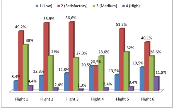
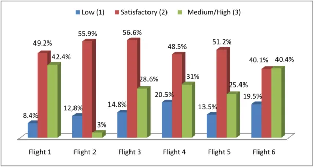
The original measures correspond to the score (in a four point ordinal scale) of each flight mission (flights one to six). Figure 3 shows the results per flight (%), demonstrating that the score 2 (Low) is the most frequent one (see also Table 4).

Figure 3 – Scores obtained in the selection flights.

Flight 1 Flight 2 Flight 3 Flight 4 Flight 5 Flight 6 8,4% 12,8% 14,8% 20,5% 13,5% 19,5% 49,2% 55,9% 56,6% 20,5% 51,2% 40,1% 38% 29% _27,3% 28,6% 32% 28,6% 4,4% 2,4% 1,3% 2,4% 3,4% 11,8% 1 (Low) 2 (Satisfactory) 3 (Medium) 4 (High)

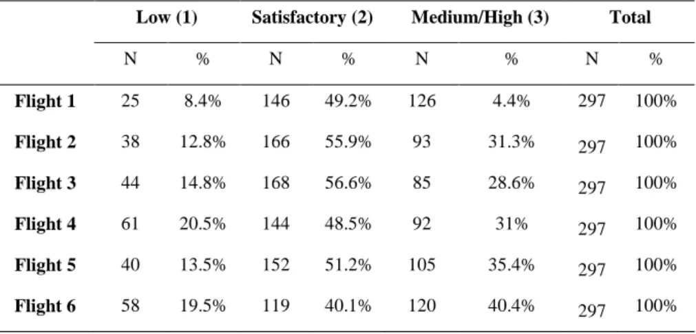
Table 4 – Flight scores frequencies.

Low (1) Satisfactory (2) Medium (3) High (4) Total

N % N % N % N % N % Flight 1 25 8.4% 146 49.2% 113 38% 13 4.4% 297 100% Flight 2 38 12.8% 166 55.9% 86 29% 7 2.4% 297 100% Flight 3 44 14.8% 168 56.6% 81 27.3% 4 1.3% 297 100% Flight 4 61 20.5% 144 48.5% 85 28.6% 7 2.4% 297 100% Flight 5 40 13.3% 152 51.2% 95 32% 10 3.4% 297 100% Flight 6 58 19.5% 119 40.1% 85 28.6% 35 11.8% 297 100%

As we can see in Figure 3 and Table 4, category 4 (High) has few observations so the original scale was aggregated into three categories (see Figure 4 and Table 5): Low (1), Satisfactory (2), and Medium/High (3).

Figure 4 – Recoded scores obtained in the selection flights.

Flight 1 Flight 2 Flight 3 Flight 4 Flight 5 Flight 6 8.4% 12,8% 14.8% 20.5% 13.5% 19.5% 49.2% 55.9% 56.6% 48.5% 51.2% 40.1% 42.4% 3% 28.6% 31% 25.4% 40.4% Low (1) Satisfactory (2) Medium/High (3)

Low (1) Satisfactory (2) Medium/High (3) Total N % N % N % N % Flight 1 25 8.4% 146 49.2% 126 4.4% 297 100% Flight 2 38 12.8% 166 55.9% 93 31.3% ₂₉₇ 100% Flight 3 44 14.8% 168 56.6% 85 28.6% ₂₉₇ 100% Flight 4 61 20.5% 144 48.5% 92 31% ₂₉₇ 100% Flight 5 40 13.5% 152 51.2% 105 35.4% ₂₉₇ 100% Flight 6 58 19.5% 119 40.1% 120 40.4% ₂₉₇ 100%

We can see (Figure 4) that data proportions for Low grade (coded as 1) increased from time measurement 1 (flight 1) to time measurement 4 (flight 4). This can be due to the increasing operations complexity required from the pilot applicants during the flights. Or, in another way, it may suggest that if one has a good grade in a first flight, the tendency is to obtain worst results in the subsequent flights.

In what refers to category 2 – Satisfactory grade, the applicants are considered to have a reasonable performance at the flights. This is considered a positive evaluation, they still perform some mistakes in their flights. There exists an increasing tendency from flight 1 to flight 3, and after flight 5 the data proportions for this category decrease.

At last, we can see that the data proportion of pilot applicants who performed Medium/High grades decreases from flight 1 to flight 3, and increases from flight 3 onwards.

Looking at Figure 4, we can assume that category 1 (Low) and 3 (medium/high) have an increasing tendency throughout the six assessments in opposition to category 2 (satisfactory) that has a decreasing tendency.

Table 6 – Summary of categorical data proportions.

Flight 1 Flight 2 Flight 3 Flight 4 Flight 5 Flight 6

Category 1 0.084 0.128 0.148 0.205 0.135 0.195

Category 2 0.492 0.559 0.566 0.485 0.512 0.401

Table 6 presents the summary of categorical data proportions. It is possible to see that the category 2 is the most frequent one for all flights, with exception of flight 6.

3.3.3 Covariates

The psychological evaluation phase to select all the candidates who join the requisites is defined in the psychological profile for the PILAV (Pilot Aviator). The psychological evaluation is based on a traditional selection procedure that consists in the application of tests, group dynamics and psychological interview.

The psychological evaluation intends to evaluate three main psychological dimensions:

a) Perceptive-cognitive dimension: evaluation of cognitive-perceptive aptitudes, through computerized tests standardized for the population in study;

b) Psychomotor dimension: evaluation of psychomotor aptitudes through computerized tests;

c) Personality and motivation dimension: evaluation based on simultaneously or separately use from the personality questionnaires, projective tests, group dynamics and individual interviews.

3.3.3.1 Personality and Motivation Dimension

The evaluation of this dimension is based on personality questionnaires, projective tests, group dynamics and psychological interviews. This dimension is operationalized in the classification of 12 factors (in a five-point scale) described in Table 7.

Factor Description

Contact and Presentation

- Courtesy, respect and education

- Availability, attention and sense of opportunity - Poise and hygiene

- Clothing and appropriate "accessories"

Communication

- Attitude and posture in favor of communication - Fluent and structured speech

- Good elocution (diction, volume ...) - Conviction and persuasion

Interpersonal relationships and teamwork - Empathy, assertive

- Good listener, sensitive, flexible

Maturity

- Capacity for reflection and preparation before the situations

- Adaptability and flexibility

- Internal locus of control, based on a set of principles and values

Emotional stability - _- Stability in the emotional-affective dimension _{Self-control in situations of pressure, or stress} evaluation

Activity level - _- High general activity _{Diverse interests and activities} - Good occupation of leisure

Initiative

- Strong presence

- Conviction and security in defense of their opinions

- Initiative

Persistence and combativeness

- Persistence in pursuit of its objectives and activities

- Proactive behavior

- Pragmatic commitment and investment in the emotional tasks (ability to delay the reward)

Decision and practical intelligence

- Determined and decided - Pragmatic

- Objectivity in the trial and mental agility - Good ability to react to pressure

Leadership

- Determination, initiative and persuasion - It is followed by others

- Ability to coordinate and guide a group - Team spirit

- Available and flexible to the other

Habits and attitudes

- Habits and positive attitudes towards: military status and situation of war, military commitments - Good attitude towards study

- Good occupation of leisure - Regular physical activity Motivation - _- Information about the PoAfA _{Enthusiasm and conviction.}

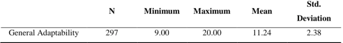
Based on all these items the applicant obtains a global score – General Adaptability - that ranges from 1 to 20 (1-3: Unfavorable; 4-7: Strong reservations; 8-9: Acceptable with reservations; 10-11: Acceptable with minor reservations; 12-14: Acceptable; 15-17:

Favorable; and 18-20: Very positive). This score measures the personality and motivation dimension and aims to prognostic the adaptation of the individuals. Table 8 depicts the descriptive statistics for General Adaptability. The mean is 11.24 (SD = 2.38; min = 9; max = 20).

Table 8 – Descriptive statistics for General Adaptability.

N Minimum Maximum Mean Std.

Deviation

General Adaptability 297 9.00 20.00 11.24 2.38

3.3.3.2 Perceptive-cognitive and Psychomotor Dimension

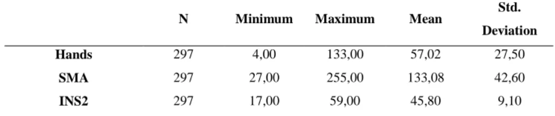
The perceptive-cognitive and psychomotor dimensions were assessed at the Psychometric Laboratory of the Portuguese Air Force in a total of 13 tests. Variables included in this study were based on two rules: (a) showed no missing values; (b) proved to be predictors of flight performance in previous validity studies (Bártolo-Ribeiro et al., 2004). Hence, the variables included in this study were INS2 (perceptive-cognitive dimension), SMA (psychomotor dimension), and Hands (perceptive-cognitive dimension). The descriptive statistics are depicted in Table 9.

a) Hands: This test requires the candidate to use an audio search message to scan visual objects and declare how many of those objects meet that search message. This task requires the translation of verbal information into visual information, and while correlated with spatial tests, is essentially a basic working memory task testing how quickly someone can move from verbal to visual information and make an accurate decision (Figure 5).

Figure 5 – Hands (spatial aptitude test).

b) Instruments Interpretation (INSB1 and INSB2): Spatial aptitude, information processing; this is a test of the candidate’s spatial visualization ability using spatial, numerical, and verbal information. The test is based on the aviation board panel (Figure 6).

Part 1 presents six aircraft instruments (altimeter, artificial horizon, airspeed, vertical speed, compass, and turn & bank) on the top half of the screen, whilst in the bottom half there are five verbal descriptions about the aircraft’s orientation. The candidate must inspect the instrument readings and select the description that corresponds to the readings.

Part 2 presents line drawings of aircraft in five different orientations and two of the instruments used in Part 1 (artificial horizon and compass). The candidate must inspect the instrument readings and identify which of the five aircraft orientations accurately corresponds to the instrument readings.

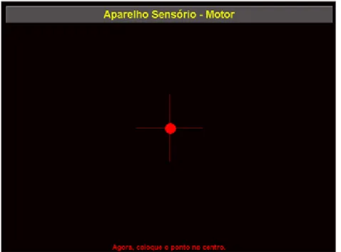
c) SMA – Sensory Motor Apparatus: multi-limbic motor coordination; SMA is a compensatory tracking test that measures eye-hand-foot coordination (psychomotor ability). The candidate uses a joystick and rudder pedals to move a pointer both horizontally and vertically on a visual display unit. Performance on the test is assessed using an error score (Figure 7).

Figure 7 – Sensory Motor Apparatus.

Table 9 depicts the descriptive statistics for the three variables (perceptive-cognitive and psychomotor dimension). For each test is presented the mean, standard deviation and the minimum and maximum value obtained at each test.