Multiple imputation of missing categorical data using latent class models: State of the art

Multiple Imputation of Missing Categorical

Data using Latent Class Models: State of the

Art

Davide Vidotto

1

, Jeroen K. Vermunt

2

& Maurits C. Kaptein

3

Abstract

This paper provides an overview of recent proposals for using latent class models for the multiple imputation of missing categorical data in large-scale studies. While latent class (or finite mixture) modeling is mainly known as a clustering tool, it can also be used for density estimation, i.e., to get a good description of the lower- and higher-order associations among the variables in a dataset. For multiple imputation, the latter aspect is essential in order to be able to draw meaningful imputing values from the conditional distribution of the missing data given the observed data.

We explain the general logic underlying the use of latent class analysis for multiple imputation. Moreover, we present several variants developed within either a frequentist or a Bayesian frame-work, each of which overcomes certain limitations of the standard implementation. The different approaches are illustrated and compared using a real-data psychological assessment application.

Keywords: latent class models, missing data, mixture models, multiple imputation.

1_{Correspondence concerning this article should be addressed to:Department of Methodology and Statistics,}

Tilburg University, PO Box 90153, 5000 LE Tilburg, The Netherlands; email:[email protected]

2_{Department of Methodology and Statistics, Tilburg University}

Introduction

Social and behavioral science researchers often collect data using tests or questionnaires consisting of items which are supposed to measure one or more underlying constructs. In a psychology assessment study for example, this could be constructs such as anxiety, extraversion, or neuroticism. A very common problem is that a part of the respondents fail to answer all questionnaire items (Huisman, 1998), resulting in incomplete datasets. However, most of the standard statistical techniques can not deal with the presence of missing data. For example, computation of Cronbach’s alpha requires that all variables in the scale of interest are observed.

Various methods for dealing with item nonresponse have been proposed (Little & Rubin, 2002; Schafer & Graham, 2002). Listwise and pairwise deletion, which simply exclude units with unobserved answers from the analysis, are the most frequently used in psychological research (Schlomer, Bauman, & Card, 2010). These are, however, also the worst methods available (Wilkinson & Task Force on Statistical Inference, 1999): they result in loss of power and, unless the strong assumption that data are missing

completely at random(MCAR)1is met, they may lead to severely biased results. Due to their simplicity and their widespread inclusion as standard options in statistical software packages, these methods are still the most common missing data handling techniques (Van Ginkel, 2007).

Methodological research on missing data handling has lead to two alternative approaches that overcome the problems associated with listwise or pairwise deletion:maximum like-lihood for incomplete data(MLID) andmultiple imputation(MI). Under the assumption that the missing data aremissing at random(MAR), the estimates of the statistical model of interest (from here on also referred to as the substantive model) resulting from MLID or MI have the desirable properties to be unbiased, consistent, and asymptotically normal (Roth, 1994; Schafer & Graham, 2002; Allison, 2009; Baraldi & Enders, 2010). MLID involves estimation the parameters of the substantive model interest by maximizing the incomplete-data likelihood function. That is, the likelihood function consisting of a part for the units with missing data and a part for the units with fully observed data. While in MLID the missing data and the substantive model are the same, in MI (Rubin, 1987) the missing data handling model (or imputation model) and the substantive model(s) of interest can and will typically be different. Note that unlike single value imputation, MI replaces each missing value withm>1 imputed values in order to be able to account

1_{According to Rubin’s (1976) classification, a missing data mechanism is said to be: (a) MCAR, when the}

for the uncertainty about the missing information. In practice, applying MI yieldsm

complete datasets, each of which can be analyzed separately using the standard statistical

method of interest, and where themresults should be combined in a specific manner.

For more details on MI, we refer to Rubin (1987), Schafer (1997), and Little and Rubin (2002).

For continuous variables with missing values, Schafer (1997) proposed using the multi-variate normal MI model, which has been shown to be quite robust to departures from normality (Graham & Schafer, 1999). Items of psychological assessment questionnaires, however, are categorical rather than continuous variables. For such categorical data, Schafer (1997) proposed MI with log-linear models, which can capture the relevant associations in the joint distribution of a set of categorical variables and can be used to generate imputation values. However, log-linear models for MI can only be applied when the number of variables is relatively small, as the number of cells in the multi-way cross-table that has to be processed increases exponentially with the number of variables (Vermunt, Van Ginkel, Van der Ark, & Sijtsma, 2008).

An alternative MI tool is offered by the sequential regression modeling approach, which

includesmultiple imputation by chained equation(MICE) (Van Buuren & Oudshoorn,

1999). This is an iterative method that involves estimating a series of univariate regression models (e.g., a series of logistic or polytomous regressions in the case of categorical variables), where missing values are imputed (variable by variable) based on the current regression estimates for dependent variable concerned. The idea of MICE is that the sequential draws from the univariate conditional models are equivalent to or at least a good approximation of draws from the joint distribution of the variables in the imputation model. Despite of being an intuitive and practical method, also MICE has certain limitations. First, there is no statistical support that missing data draws converge to the posterior distribution of the missing data. Second, by default, MICE only includes the main effects in the regression equations, which risks to not pick up higher-order interactions among the variables. Furthermore, whereas the method allows including higher-order interactions, this can be a fairly difficult and time-consuming task when the number of variables in the imputation model is large (Vermunt et al., 2008).

Vermunt et al. (2008) proposed an imputation model for categorical data based on a

maximum likelihood finite mixture orlatent class(LC) model. LC models for MI seem

appropriate for datasets coming from large-scale assessment studies, where the number of variables can be large and where association structures can be complex.

Recently, Van der Palm, Van der Ark, and Vermunt (2013b) proposed a variant of the LC model called thedivisive latent class model, which can be used for density estimation and MI. Compared to the standard LC model, this approach reduces computing time enormously. Instead of using frequentist maximum likelihood methods, LC analysis can also be implemented using a Bayesian approach as shown among others by Diebolt and Robert (1994). An interesting recent development concerns the use of Bayesian nonparametric methods for MI. More specifically, inspired by Dunson & Xing’s (2009)

mixture of independent normal distribution with Dirichlet process prior, Si and Reiter (2013) proposed using a nonparametric finite mixture model for MI in a Bayesian framework.

The aim of this paper is to offer a state-of-the-art overview of MI using LC analysis in which we show similarities and differences and discuss pros and cons of the recently proposed frequentist and Bayesian approaches. The remainder of the article is structured as follows. In Section 2, the basic LC model is introduced and its use for MI is motivated. Section 3 describes the four different LC MI methods in more detail. Section 4 illustrates the use the four types LC MI methods in a real-data example, and also compares the obtained results with those obtained with listwise deletion and MICE. Section 5 discusses our main findings, gives recommendations for those who have to deal with missing data, and lists topics for further research.

Latent Class models and Multiple Imputation

Latent Class Analysis for Density Estimation

The latent class model (Lazarsfeld, 1950; Goodman, 1974) is a mixture model which describes the distribution of categorical data. Mixture models are flexible tools that allow modelling the association structure of a set of variables (their joint density) using a finite mixture of simpler densities (McLachlan & Peel, 2000). In LC analysis, each latent class (or mixture component) has its own specific multinomial density, defining the probability of having a specific response pattern. The estimated overall density is obtained as a weighted average of the class-specific densities. An important assumption of LC analysis islocal independence(Lazarsfeld, 1950), according to which the scores of different items are independent of each other within latent classes.

yi j be the score of the i-th person on the j-th categorical item belonging to an×J data-matrixY (i=1, ...,n, j=1, ...,J),yyy_iiitheJ-dimensional vector with all scores of personi, andxia discrete (unobserved) latent variable withKcategories. In the LC model, the joint densityP(yyy_iii;πππ)has the following form:

P(yyy_iii;πππ) = K

∑

k=1

P(xi=k;πππx)P(yyyiii|xi=k;πππy)

= K

∑

k=1

P(xi=k;πππx) J

∏

j=1

P(yi j|xi=k;πππyj). (1)

The LC model parametersπππcan be partitioned into two sets: the latent class proportions (πππx) and class-specific item response probabilities (πππy), where the latter contains a sepa-rate set of parameters for each item (πππyj). The fact that we are dealing with a mixture

distribution can be seen from the fact that the overall density is obtained as a weighted sum of theKclass-specific multinomial densitiesP(yyy_iii|xi=k;πππy), where the latent pro-portions serve as weights. Moreover, in (1) the local independence assumption becomes visible in the product over theJindependent multinomial distributions (conditional on thek-th latent class).

By setting the number of latent classes large enough, LC models can capture the first,

second, and higher-order moments of theJresponse variables (McLachlan & Peel,

2000), that is, univariate margins, bivariate associations, and higher-order interactions when dealing with categorical variables (Vermunt et al., 2008). Moreover, because of the local independence assumption, it is possible to obtain estimates of the model parameters also whenJis very large.

A quantity of interest when using LC models is the units’posterior class membership

probabilities, i.e., the probability that a unit belongs to thek-th class given the observed data patternyyy_iii. It can be defined through the Bayes’ theorem as follows:

P(xi=k|yyyiii;πππ) =

P(xi=k;πππx)P(yyyiii|xi=k;πππy)

P(yyy_iii;πππ) .

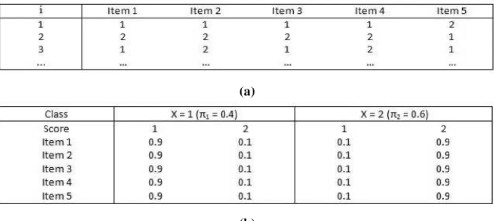
As an example, suppose we have a data-matrixY forJ=5 binary variables, where

the first 3 observations have the observed patterns presented in Figure 1a. Suppose

furthermore that we specified a 2-class model (K=2) and obtained the parameter

(a)

(b)

Figure 1:(a) Example of observed data-matrix Y for J=5dichotomous items and observed patterns yifor

i={1,2,3}.

(b) Example of 2-class LC model parameters: latent probabilitiesπx(on the top) and conditional

probabilitiesπyj(in the body of the table).

equals 0.997, whereas for the second observation the class 2 posterior probability

P(x2=2|yyy222;πππ)equals 0.999. The third unit has posteriorsP(x3=1|yyy333;πππ) =0.86 and

P(x3=2|yyy333;πππ) =0.14.

Multiple Imputation using LC Models

In a standard LC analysis, the aim is to find a meaningful clustering with a not too large number of well interpretable clusters. In contrast, when used for imputation purposes, the LC model is “just” a device for the estimation ofP(yyy_iii;πππ). In other words, in MI, LC models do not need to identify meaningful clusters, but instead should yield an as good as possible description for the joint density of the variables in the imputation model. This means that issues which are problematic in a standard LC analysis, such as nonidentifiability, parameter redundancy, overfitting, and boundary parameters, are less of an issue in a MI context. The main thing that counts is whetherP(yyy_iii;πππ)is approximated well enough in order to be able to generate as good as possible imputations based onP(yyy_i,mis|yyyi,obs).

model, (b) capturing some sample specific variability (namely overfitting the data) is not problematic in this context, because the aim is to reproduce a sample even with its specific fluctuation, while ignoring certain structures of the data (underfitting) can cause important associations between the variables to be ignored, (c) unidentifiability is not an issue either, inasmuch the quantity of interestP(yyy_iii;πππ)is uniquely defined even when the values ofπππare not, and (d) obtaining a local maximum of the log-likelihood function, instead of a global maximum, is also not a problem since the former may provide a representation ofP(yyy_iii;πππ)that is approximately as good as the one provided by latter.

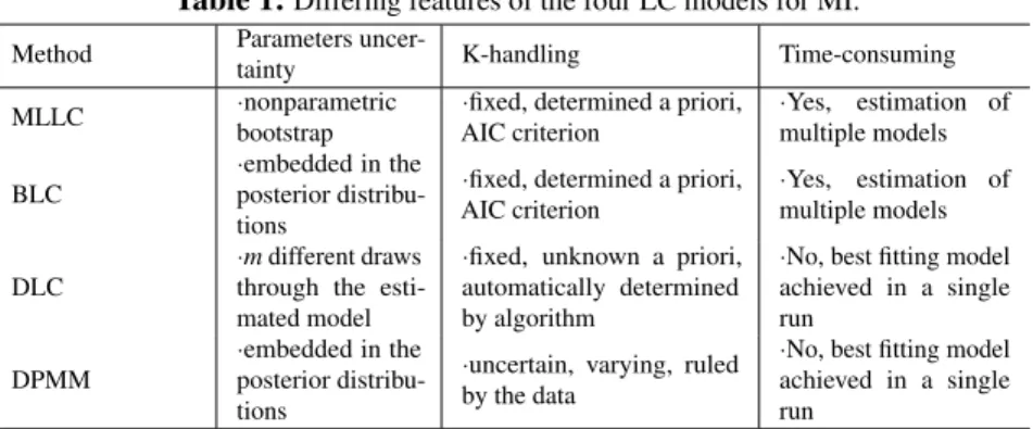
Once the LC model has been estimated using an incomplete dataset, it is possible to

perform MI by randomly drawingmimputations for each nonresponse from the posterior

distribution of the missing values given the observed data and the model parameters. To make this clearer, let us return to the small example introduced in the previous section. Suppose now we also have missing values as shown in Figure 2, and that under this new scenario the resulting LC 2-class model is again the one with the parameter values presented in Figure 1b. Withyyy_i,obswe denote the observed part of the response pattern for personi, while the unknown part, marked with “?", is denoted byyyy_i,mis. LC model parameter (πππ) estimation and inference can be achieved with only the observed information,yyy_i,obs. As shown among others by Vermunt et al. (2008), the probability

P(yyy_i,mis|xi=k;πππy)cancels from the (incomplete data) log-likelihood function that is maximized, which implies that each subject contributes only to the parameters for the variables which are observed2.

Once the model has been estimated, the aim of MI is to generate an imputation for each “?" in the dataset by sampling fromP(yyy_i,mis|yyy_i,obs;πππ). This requires two draws: the first assigns a class to each unit using the posterior membership probabilities given

yyy_i,obs. Unit 1, for instance, has now a probability equal toP(x1=1|yyy1,obs;πππ) =0.98

to belong to class 1 andP(x1=2|yyy1,obs;πππ) =0.02 to belong to class 2. Once the

class membership has been established, “?" in itemjis replaced by drawing from the conditional multinomial distribution of j-th item in that class. If, in the previous step, the first unit was allocated to the first class, then the missing value of Item 4 will be replaced by the value 1 with probability 0.9 and by the value 2 with probability 0.1. The uncertainty about the imputations is accounted for by repeating this procedurem>1 times for each unit with at least one missing value.

LC models can also be implemented within a Bayesian framework, which involves specifying prior distributions for the class proportions and the class-specific response probabilities. Two kinds of priors can be applied: a Dirichlet distribution or a Dirichlet

2_{In Vermunt et al. (2008) and Van der Palm, Van der Ark, and Vermunt (2014) the procedure is given for}

Figure 2:Example of data-matrix Y for J=5dichotomous items and i={1,2,3}, with both observed and missing data (the latter marked by "?").

Process prior. The Dirichlet distribution, used as prior for the multinomial conditional distributions or for the multinomial latent distribution of standard Bayesian LC models, is suited for modelling multivariate quantities that lie in the interval (0,1) and that sum to 13. In the Dirichlet process approach, on the other hand, the number of latent classes becomes uncertain, and a baseline distribution is used as prior expectation density. A concentration parameter (α) rules the concentration of the prior forxiaround the baseline density: whenα is large, the prior ofxi is highly concentrated around the expected baseline (the latent classes will tend to have equal sizes), while for smallα there is a larger departure from the baseline (few classes will have most of the probability mass) (Congdon, 2006).

In a frequentist setting, maximum likelihood (ML) estimation is typically performed using an EM algorithm (Dempster, Laird, & Rubin, 1977), whereas in a Bayesian framework, MCMC algorithms such as the Gibbs sampler are used (Geman & Geman, 1984; Gelfand & Smith, 1990). In mixture models, the Gibbs sampler iterations contain a Data Augmentation step in which units are allocated to latent classes. The Data Augmentation (DA) algorithm (Tanner & Wong, 1987) can be seen as a Bayesian version of the EM algorithm, which can be used for the estimation of Bayesian LC models. DA is particularly suitable also for MI computation as it also involves imputing the missing data given the current state of the model parameter as one of the steps. Tanner and Wong (1987) showed that under certain conditions, the algorithm converges to the true posterior distribution of the unknown quantities of interest. Themimputations are

obtained by drawingmimputed scores from the posterior distribution of the missing

values. A description of both the Gibbs sampler and the DA algorithm is provided in Appendix A.2.

Four Different Implementions of Latent Class Multiple Imputation

In this section we present four different implementations of LC models for MI: the Maximum Likelihood LC model (MLLC), the standard Bayesian LC model (BLC), the Divisive LC model (DLC), and the Dirichlet Process Mixture of Multinomial distribu-tions (DPMM). These four models share the characteristics of the LC model mentioned in the previous section, which make that each of them can serve an excellent tool for the MI of large datasets containing categorical variables.

These four types of LC models, however, also differ in a number of respects. First, they differ in the way in which they deal with the uncertainty about the model parameters. Note that taking into account this uncertainty during the imputation is a requirement for valid inference with a multiple imputed data set. The two frequentist models (MLLC and DLC) resort either on a nonparametric bootstrap or on different draws of class membership and missing scores, whereas the two Bayesian methods (BLC and DPMM) automatically embed parameter uncertainty by sampling the parameters from their posterior distribution.

Second, the four methods differ in the way they select the number of classesK. While the standard implementation of the LC model (MLLC and BLC) requires estimating and testing a series of models with different numbers of classes using some fit measure (e.g., the AIC), in DLC and DPMM the number of classes is determined in an automatic manner. In DPMM the number of latent classes is treated as a model parameter, while

for the other three types of modelsKis fixed though unknown.

Lastly, the four methods differ in terms of computational efficiency. Note that the main factors affecting computation time are the sample sizen, the number of classesK, and the

number of variablesJ. While MLLC and BLC require estimating models with different

Fixed K, Frequentist: the Maximum Likelihood LC Model

The MLLC approach uses a nonparametric bootstrap4in order to take into account the

uncertainty about the imputation model parameter estimates, which is a requirement for valid post-imputation inference. Specifically, imputation using MLLC proceeds as follows: first,mnonparametric bootstrap samplesY_l∗(l=1, ...,m) of sizenare obtained from the original datasetY; second, the LC model is estimated for eachY_l∗, providing

mdifferent sets of parametersπππl_{; third, the original dataset is duplicatedmtimes and} for thel-th dataset the set of parametersπππl_{is used to impute the missing values from}

P(yyy_i,mis|yyyi,obs;πππl).

To describe the joint distribution of the data as accurately as possible,Kis selected based on penalized likelihood statistics, such as the AIC (Akaike Information Criterion) or the BIC (Bayesian Information Criterion) index. In MI, the AIC criterion is preferable over BIC since it yields a larger number of classes; nevertheless, an even higherKthan the one indicated by the AIC index may be used, since, as already noticed, the risk of overfitting in the MI context is less problematic than the risk of underfitting.

Though Vermunt et al. (2008) showed that the performance of MLLC is similar to both

ML for incomplete dataandMI using a log-linear model, in terms of parameter bias, some issues with respect to the model-fit strategy remain; in order to select the optimal

Kvalue according to the AIC index, in fact, one needs to estimate a 1-class model, a 2-class and so on, until the best fitting model has been found5. It will be clear that this approach may be time-consuming, especially when used with large data sets.

MI through MLLC is available in software such as LatentGOLD (Vermunt & Magidson, 2013), which includes a special option for MI. In R, LC analysis can be performed with the package poLCA (Linzer & Lewis, 2014). This package could be used to implement the MI procedure described above.

4_{The nonparametric bootstrap (Efron, 1979) is a technique that allows reproducing the distribution of some}

specific parameter by resampling observations from the original sample multiple times with replacement; in such a way, the original sample is treated as the population of interest. Through this procedure, which is useful when the theoretical distribution of the parameters of interest is difficult to derive, uncertainty about the model parameters can be inferred.

5_{Rather than starting with a one class model and subsequently increasing the number of classes, alternative}

Fixed K, Bayesian: the Bayesian LC Model

While in the frequentist framework a nonparametric bootstrap is needed to account for parameter uncertainty, when using a Bayesian MCMC approach parameter uncertainty is automatically accounted for. More specifically, Rubin (1987) recommended using Bayesian methods in order to obtain proper imputations, which fully reflect the

uncer-tainty about the model parameters and which are draws from theposterior predictive

distributionof the missing data. Vermunt et al. (2008) mentioned the possibility to implement their approach using a Bayesian framework. Si and Reiter (2013) present the Bayesian LC (BLC) model as a natural step to go from the MLLC to the DPMM MI approach. Therefore, though the BLC model has not been proposed explicitly for MI, we present it here as one of the possible implementations of LC-based MI. As in the frequentist case, standard parametric BLC analysis requires that we first determine the

value ofK, for example, using the AIC index evaluated by ML estimation. Therefore,

also with this approach, determining the number of classes may be rather time consuming in larger data sets.

For the distribution ofπππxthe prior will typically be aK-variate Dirichlet distribution (if

K=2 this is equal to a Beta distribution), whereas for the conditional probabilitiesπππyj, a

Dirichlet prior for each j=1, ...,Jandk=1, ...,K, with number of components equal to the number of categories of the j-th variable, is assumed. Setting weakly informative prior distributions helps the posterior distribution ofπππ to be data dominated. For the Dirichlet distribution, an uniform prior is achievable by initializing all its parameters to 16. Within the latent classes, the conditional probabilities are initialized to be equal to the observed marginal frequencies of the scores of each variable. Also, for MI, nonresponses are initialized with a random draw from the observed frequency distribution of the variables with missing values. Once the first set ofπππxhas been drawn from the Dirichlet prior, the Gibbs sampler proceeds as follows. First, each unit is assigned to a latent category by drawing from the posterior membership probabilitiesP(xi=k|yyyiii;πππ); second, the parameters of the Dirichlet distribution forπππxare updated: this is done by adding the number of units dropped in thek-th latent class to the starting value of thek-th parameter (that is 1 in the case of a weakly informative prior). From this updating, a new value ofπππxis extracted. Third, the parameters of the Dirichlet distributions ofπππyj are in turn

updated in an analogue way: the number of units which take on one of the possible observed values of the j-th variable and dropped into thek-th latent class is added to the initial parameter value of the category concerned of the j-th Dirichlet prior of the

6_{This is equivalent to a prior sample size equal to the number of components of the Dirichlet distribution.}

k-th latent component (again, this is 1 in the case of a weak prior); after the updating, a new value ofπππyj is drawn. The fourth, and last, step is the imputation step: given the

valuexi=kof each unit (resulting from the first step), and the new set of probabilities

π π

πyj, a new score foryij,misis drawn fromP(yij|xi=k;πππyj). Steps 1-4 are repeated until

convergence is reached. Appendix B.1 gives a formal description of these steps.

A BLC model can be estimated in R through the package “BayesLCA" (White & Murphy, 2014).

Unknown K, Frequentist: the Divisive LC Model

The main problem of the standard LC approach is that it uses a substantial amount of computation time to estimate multiple models with increasing number of classes to determine the value ofK. Divisive latent class (DLC) models (Van der Palm et al., 2013b) overcome this problem by breaking down the global estimation problem into a series of smaller local problems. The DLC model incorporates an algorithm that increases the number of latent classes within a single run until the possible improvements in model fit have been achieved. This implies that the best fitting model is found in a single estimation run. The DLC model has been developed by Van der Palm et al. (2013b, 2014) for density estimation and MI purposes, while a substantive interpretation of the resulting LC parameters is still unexplored.

The DLC algorithm involves evaluating a series of 1-class and 2-class models. At the start, a single LC assumed to contain the whole sample is split into two latent classes if the 2-class model improves the model fit sufficiently (for instance, in terms of log-likelihood). If this is the case, every unit will have a probability of belonging to each of the two latent classes, which corresponds to the posterior class membership probabilities. Using these posterior probabilities, two fuzzy subsamples are created. In the following step, these two new latent classes are checked separately to establish whether a further split into 2 classes, within each subsample improves the model fit. In the next steps, this operation is repeated for each newly formed latent class, until the best model fit is achieved for every fuzzy subsample. Since a DLC model is estimated sequentially, each submodel created at stepsbuilds on the results of steps 1, ...,s−1; in such a way an

automatic estimate of the optimumKis obtained with much smaller computation time

Van der Palm et al. (2014) observed that the DLC model in combination with the non-parametric bootstrap may yield biased parameter estimates in a subsequent substantive analysis. Therefore, they proposed implementing the actual MI procedure in slightly different from MLLC, while still taking into account the uncertainty about the imputation model parameters. First, the DLC model and its parametersπππ is estimated using the original dataset; second, the posterior membership probabilitiesP(xi=k|yyyi,obs;πππ)are

computed; third, the original dataset is duplicatedmtimes; fourth, theP(xi=k|yyyi,obs;πππl)

are used to assignmtimes a latent class to each respondent; last, for each missing

value of unitiin item j,mmissing scores are sampled using the conditional response probabilitiesP(yi j|xi=k;πππ).

The Latent GOLD software allows performing DLC-based MI, while to our knowledge currently there is no R package that implements the DLC approach.

Variable K, Bayesian: Dirichlet Process Mixture of Products of Multinomial Distributions

Even if the AIC index provides a sufficiently large number of mixture components,

once the value ofK is determined uncertainty aboutK is ignored when generating

the imputations. This counters Rubin’s (1987) suggestion to account for all possible uncertainties about the imputation model parameters in order to avoid underestimation of the variances of the substantive model parameters (Si & Reiter, 2013). The Dirichlet process mixture of products of multinomial distributions (DPMM) overcomes the need of an ad hoc selection of a fixedKand, moreover, automatically deals with the uncertainty about this parameter. This happens by assuming that in theory there is an infinite number of classes (K= +∞), but letting the data fill only a smaller number of components that is actually needed. A simulation study by Si and Reiter (2013) showed that DPMM MI may outperform MICE in terms of bias and confidence interval coverage rates of the parameters of a substantive model.

DPMM offers a full Bayesian modeling approach for high-dimensional categorical data. Similarly to BLC, DPMM can be estimated through the Gibbs sampler. One of the possible conceptualization of the Dirichlet process which serves as a prior for the mixture proportionsπππxis thestick-breaking process(Sethuraman, 1994; Ishwaran & James, 2001). In this formulation, an element ofπππx, sayπk (k=1, ...,+∞), is assumed to take on the formπk=Vk∏h<k(1−Vh)for eachk, where everyVkis drawn from a Beta distribution with parameters(1,α). Here,α, the concentration parameter of the process,

is allowed to vary according to a Gamma distribution with parameters (a,b). The

to set weakly informative priors for the model parameters; Dunson & Xing’s (2009) suggestion for weak priors is to initializeα to be equal to 1 and set the parameters of its Gamma distribution toa=b=0.25. This allows eachVkto be uniformly distributed in the (0,1) range, whereas the Dirichlet priors of the conditional distributions can be made uniform by setting all their parameters to 1 (as we already saw for the BLC approach). Since the stick-breaking specification of the Dirichlet process incentivizes the size of each latent classπkto decrease stochastically withk, this model tends to put meaningful posterior probabilities on a limited number of components automatically determined by the data. When the concentration parameterα is small, in fact, most of the probability mass is assigned to the first few components, with the number of significant components increasing asαincreases. As a consequence, there will be a finite number of classes with a meaningful size, while the classes with a negligible probability mass will be ignored.

Since working with an infinite number of classes is impossible in practice, Si and Reiter (2013) proposed truncating the stick-breaking probabilities at an (arbitrarily) largeK∗, but not so large as to compromise the computing speed. If, after running the MCMC chain, significant posterior masses are observed for allK∗components, the truncation limit should be increased. As for the BLC approach, conditional probabilities of theJ

variables within each latent class are initialized with the observed frequencies and, for MI, missing data are initialized too with draws from these frequency tables. The Gibbs sampler is then performed as follows. First, each unit is assigned to a latent category by drawing from the posterior membership probabilitiesP(xi=k|yyyiii;πππ); second,Vk (k=1, ...,K∗−1 because of the truncation) are drawn from a Beta distribution, whose first parameter is updated by adding the number of units allocated in thek-th latent class to its initial value (set to 1), whereasαis updated by adding to it the number of units assigned to the latent classes which go fromk+1 toK∗; after settingVK∗=1, eachπ_k

is calculated through the formulaπk=Vk∏h<k(1−Vh); in the third step the parameters of the conditional Dirichlet distributions ofπππyj are updated by adding the number of

units, which take one of the possible observed values of thej-th variable and are dropped into thek-th latent class, to the initial parameter value of the related component of that distribution; after the updating, a new value ofπππyj is drawn; fourth, a new value for

the concentration parameterα is drawn from the Gamma distribution with parameters

updated asa+K∗−1 andb−log(πK∗); fifth, the imputation step analogue to BLC is performed. Steps 1-5 are repeated until convergence is reached. For a formal description of the algorithm, see Appendix B.2.

To our knowledge no off-the-shelf software is currently available that enables estimation of the DPMM model. We implemented a custom routine in R to fit the model. The R-code is available from the corresponding author upon request7.

Table 1:Differing features of the four LC models for MI.

Method Parameters

uncer-tainty K-handling Time-consuming

MLLC ·nonparametric

bootstrap

·fixed, determined a priori, AIC criterion

·Yes, estimation of multiple models

BLC

·embedded in the posterior distribu-tions

·fixed, determined a priori, AIC criterion

·Yes, estimation of multiple models

DLC

·mdifferent draws through the esti-mated model

·fixed, unknown a priori, automatically determined by algorithm

·No, best fitting model achieved in a single run

DPMM

·embedded in the posterior distribu-tions

·uncertain, varying, ruled by the data

·No, best fitting model achieved in a single run

Table 1 summarizes the main differences of the four models described in this section. In the next section, we are going to apply the LC MI models to a real-data example in order to show their working in the practice. We will examine similarities and differences between the four methods and also with listwise deletion and MICE.

Real-data Example

The KRISTA dataset (Van den Broek, Nyklicek, Van der Voort, Alings, & Denollet, 2008) contains self-reported and interviewer-rated information from 748 patients aged between 18 and 80 years who got an Implantable Cardioverter Defibrillator (ICD) in two large Dutch referral hospitals between May 2003 and February 2009. The aim of the study was to determine whether personality factors affect the occurrence of anxiety as a result of the shocks the patients gets from the ICD. We selected the items of four scales to illustrate the application of MI: Eysenck Personality Questionnaire (EPQ, 24 binary items scored 0-1, 12 of which measure patient’s neuroticism -EPQN- and the remaining 12 measure patient’s extraversion -EPQE), Marlowe Crowne Scale (MC, 30 binary items scored 0-1), State-Trait Anxiety Inventory (STAI, 20 items on a 4-point Likert scale), and Anxiety Sensitivity Index (ASI, 16 items ranging from 0 to 4). We included in the analysis also the categorical background variable Sex, yielding a total

ofJ=91 variables. After removing the persons without any observed score on the

90 questionnaire items, we have a sample size ofn=706 patients,nM=555 of which

are men andnF=151 of which are women. Although in this reduced dataset the total

percentage of missingness was very low (2.4%), it should be noticed that a method such

as listwise deletion (LD) may cause a large amount of loss of power, since about 30% of the units contained at least one missing value, resulting in onlyn∗=494 persons with fully observed information (n∗_M=400 males andn∗_F=94 women).

We also created a version of the same dataset with some extra MAR missingness8_{. The} new total rate of missingness was about 22.5%. In this new case, onlyn∗∗=109 units had a completely observed response pattern (of whichn∗∗_M =96 males andn∗∗_F =13 women) while the remainingn−n∗∗=597 cases (84.56 % of the units) had at least one missing value. This data set with a much larger percentage of missing values will be used to investigate whether and how the behaviour of the missing data models differs compared to the original low missingness situation.

Case I - Low missingness. We applied LD and MICE and the four LC MI methods to the original dataset. Subsequently, we computed the estimates of various quantities of interest for the resulting complete data sets. For the scales we selected, we obtained Cronbach’s alpha ( ˆα), the means for males and females ( ˆµMand ˆµF) and their standard

errors ( ˆσµM, and ˆσµF), the t-value of the test for assessing the hypothesis of equality of

means between men and women (against the alternative hypothesisH1: ˆµM=µˆF)and

the resulting p-value.

Note that the purpose of our example is to illustrate the use of the LC-based MI ap-proaches with a real life application. Contrary to the controlled conditions of a simulation study, we do not know the true values of the quantities of interest. Instead, we will compare the estimates obtained with different imputation methods, as well as compare the estimates obtained in the low missingness condition (Case I) with those in the high missingness condition (Case II). For elaborate simulation studies on the behavior of the LC imputation models, we refer to Vermunt et al. (2008); Van der Palm, Van der Ark, and Vermunt (2013a); Gebegziabher and DeSantis (2010); Si and Reiter (2013).

We applied MICE with its default setting using the R library (Van Buuren et al., 2014) and ran it for 15 iterations. For MLLC and BLC, we specified two kind of models,

one resulting from the selection of K based on the AIC index and the other using

an arbitrarily large value forK. Models specified through the AIC index will be

de-noted by MLLC(AIC) and BLC(AIC), while models with a largeKwill be denoted by

MLLC(large) and BLC(large). For the former, we estimated a 1-class model, a 2-class model, and so on, up to a 70-class model. The best fitting model, according to the AIC index, was the 14-class model. MLLC(large) and BLC(large) were implemented with

K=50. Furthermore, we used the 1-class MLLC model (MLLC(1), an independence

8_{For the generation of the extra missingness, we followed Brand (1999) and Van Buuren, Brand,}

model), which is in fact a random version of mean (or mode) imputation. We used the MLLC(1) model to show the consequence of using an imputation model that does not correctly model the associations between the variables in the data file. The DLC model was estimated with a decision rule based on the improvement in log-likelihood larger than 0.6·J, following Van der Palm et al.’s (2014) advice. This resulted in a model with

K=111 classes. DPMM, finally, was implemented withK∗=50 truncated components.

For BLC and DPMM, the Gibbs samplers were run withB=50000 iterations and with

the prior specifications described in Section 3.

Model-estimation and imputation was performed with LatentGOLD 5.0 (Vermunt & Magidson, 2013) for MLLC and DLC, while we implemented two routines in R 3.0.2 for the Gibbs samplers of BLC and DPMM. Following Graham, Olchowski, and Gilreath

(2007) we usedm=20 imputations for each method (including MICE). R 3.0.2 was

used to obtain estimates for the parameters of interest with LD and the MI methods (pooled estimates for the latter).

Table 2 reports ˆα, ˆµM, ˆµF, ˆσµM, ˆσµF, t-values, and p-values for each method. The ˆσµMand

ˆ

σµFobtained with the MI methods reflect both the “within imputation” and the “between

imputation” variability of the estimates of the population means. T-values were also calculated taking into account both the sources of variability. Null hypotheses rejected at the significance level of 5% are marked in boldface.

As can be seen, the estimates obtained with the different LC-MI implementations are all very similar. However, the estimates provided by the MI methods appear to differ systematically from the estimates of the LD method. For example, the ˆαestimates for the EPQN and ASI scales obtained with the MI approaches are always larger than the ones for LD, but the differences among the LC models (both frequentist and Bayesian) are very small. Also some differences between MICE and LC imputation methods can be observed. For example, the Cronbach’s alpha of the EQPN and ASI scales of MICE are not only larger than those of LD, but also somewhat larger than those of the LC methods.

Also for ˆµM and ˆµF, differences between the LC imputation models are very small.

Multiple

Imputation

using

Latent

Class

Models

559

Missing data model

Scale LD MICE MLLC(1) MLLC(AIC) MLLC(large) DLC BLC(AIC) BLC(large) DPMM EPQN 0.833 0.861 0.845 0.850 0.850 0.850 0.850 0.850 0.850 EPQE 0.873 0.865 0.860 0.864 0.863 0.864 0.863 0.863 0.862 ˆ

α MC 0.759 0.763 0.732 0.735 0.736 0.736 0.734 0.735 0.736 STAI 0.944 0.944 0.942 0.945 0.945 0.945 0.945 0.945 0.945 ASI 0.886 0.900 0.890 0.894 0.892 0.894 0.893 0.894 0.894 EPQN 8.802 8.480 8.612 8.593 8.606 8.610 8.598 8.597 8.589 EPQE 4.832 4.939 4.867 4.903 4.866 4.878 4.881 4.879 4.885 ˆ

µM MC 20.467 20.269 20.469 20.474 20.468 20.470 20.447 20.445 20.448 STAI 37.355 38.652 38.179 38.241 38.237 38.180 38.227 38.217 38.224 ASI 12.847 13.547 13.260 13.328 13.314 13.351 13.337 13.375 13.367 EPQN 8.010 7.352 7.535 7.521 7.517 7.509 7.510 7.524 7.520 EPQE 5.223 5.272 5.138 5.113 5.176 5.148 5.133 5.117 5.126 ˆ

µF MC 22.032 21.467 21.759 21.732 21.807 21.756 21.736 21.742 21.736

STAI 39.053 41.203 40.730 40.748 40.663 40.711 40.738 40.674 40.687 ASI 13.979 15.591 15.108 15.272 15.150 15.185 15.261 15.252 15.276 EPQN 0.153 0.142 0.135 0.137 0.137 0.136 0.137 0.137 0.136 EPQE 0.179 0.152 0.149 0.151 0.150 0.151 0.150 0.150 0.150 ˆ

σµM MC 0.228 0.197 0.186 0.187 0.187 0.188 0.187 0.187 0.187

STAI 0.567 0.510 0.491 0.499 0.496 0.497 0.498 0.497 0.497 ASI 0.481 0.436 0.417 0.422 0.419 0.424 0.422 0.425 0.424 EPQN 0.336 0.284 0.274 0.278 0.277 0.277 0.278 0.279 0.278 EPQE 0.356 0.273 0.262 0.264 0.264 0.266 0.266 0.265 0.263 ˆ

σµF MC 0.415 0.365 0.324 0.327 0.324 0.327 0.327 0.325 0.329

STAI 1.105 0.937 0.905 0.930 0.927 0.928 0.930 0.932 0.930 ASI 0.936 0.885 0.845 0.864 0.849 0.859 0.859 0.861 0.862 EPQN 2.226 3.638 3.642 3.577 3.631 3.685 3.632 3.562 3.566 EPQE -0.957 -1.027 -0.851 -0.654 -0.972 -0.842 -0.785 -0.744 -0.754 t-value MC -3.056 -2.809 -3.258 -3.171 -3.373 -3.222 -3.242 -3.272 -3.236 STAI -1.319 -2.333 -2.425 -2.341 -2.273 -2.368 -2.345 -2.297 -2.302 ASI -1.036 -2.140 -2.027 -2.096 -2.001 -1.977 -2.081 -2.018 -2.053 EPQN 0.026 0.0003 0.0003 0.0004 0.0003 0.0002 0.0003 0.0004 0.0004

EPQE 0.339 0.305 0.395 0.513 0.332 0.400 0.433 0.457 0.451 p-value MC 0.002 0.005 0.001 0.002 0.0008 0.001 0.001 0.001 0.001

STAI 0.188 0.020 0.016 0.019 0.023 0.018 0.019 0.022 0.022

ASI 0.301 0.033 0.043 0.036 0.046 0.048 0.038 0.044 0.040

As far as MICE is concerned, it can be seen that the difference in estimated means between MICE and LD is usually larger than the difference between LC-MI and LD.

If we look at the SE estimates, the LC-MI procedures seem to yield somewhat smaller value than MICE and LD (which is disadvantaged by a smaller sample size). Furthermore, SEs are very similar across LC methods. Differences between LD and the MI methods turn out to be important for the t-tests: while we rejected only 2 null hypotheses (EPQN and MC) with LD, we have 4 out of 5 rejections (EPQN, MC, STAI and ASI) with all MI methods investigated.

It is also possible to see from Table 2 that the independence model, MLLC(1), does not produce very different results compared to the other LC MI models. The main difference occurred in the estimates of ˆα, which are slightly lower than the Cronbach’s alpha produced by the other LC-MI methods. The other quantities do not differ much from those obtained with the others LC imputation models. Seemingly, with this low rate of missingness, it is more important to prevent deleting cases with missing values than to have "correct" imputations for the missing values.

Given the similar results produced by the MI methods, a look at the computation times in Table 3 may be useful for a further comparison. For the MLLC approach, the required computation time to estimate models with fewer classes is also reported. Estimation of MLLC models with 1 up to 70 classes took almost 13 hours. For BLC and DPMM, we report the computation time required to run the Gibbs sampler for one model. The time spent on estimating all MLLC models should be added to the computation time to run the Gibbs sampler for BLC(AIC). Running the MICE with (only) 15 iterations required about 13 hours. Among the LC imputation methods, MLLC and BLC(AIC) are more time-consuming than DLC, BLC(Large), and DPMM, which are faster and took about the same computation time, as they do not require the estimation of multiple models to find the ideal number of classes.

Case II - High missingness. Table 4 reports the estimates obtained using the KRISTA

dataset with extra (22.5%) missingness. The settings were the same as with Case I,

except for the number of classes of MLLC(AIC) and BLC(AIC), which wasK=10,

and the number of classes of DLC, which wasK=106. The LD method was applied

withn∗∗=109 persons with fully observed score patterns.

As can be seen from Table 4, the contrast between LD and the MI methods, as well as the differences between MICE, the 1-class LC model, and the other LC models, are much clearer now. This shows that the way the imputation is performed matters with larger proportions of missing values. All LC imputation methods recover ˆµMand ˆµFwell; that

Table 3:Computation time for MI using MICE and the six different LC imputation models.

Imputation model Model time Total time

MICE* / 13h05min

MLLC(AIC)** 0h58min 12h51min

MLLC(large)** 7h17min 12h51min

DLC 5h39min 5h39min

BLC(AIC)*** 6h04min 18h55min

BLC(large) 6h41min 6h41min

DPMM 6h27min 6h27min

Note: *MICE was run for 15 iterations. **MLLC models were estimated from MLLC(1) to MLLC(70). The second column shows the required time to estimate the indicated model, while the third column shows the computation time taken to estimate all the 70 models. ***For BLC, in the second column the computation time needed to run the Gibbs sampler has been reported, while in the third column the computation time of MLLC for selecting the number of classes has been added.

Also the estimated standard errors of the means, ˆσµM and ˆσµF, do not differ much from

the previous case, though they are slightly smaller than for Case I. Notice, furthermore, that the MLLC(1) model yielded standard errors that are much smaller than the other methods, showing that an under-specified model will typically underestimate variability. The t-tests with MLLC(large), BLC(large) and DPMM yielded the same conclusions as with Case I, as 4 out of 5 tests are rejected at a significance level of 5 %. MLLC(AIC), DLC, and BLC(AIC) did not reject the hypothesis of equality of means for the ASI scale, which is result of the slightly lower power in the high missingness condition. LD seems to produce very much biased means and large standard errors (the latter resulting from the strongly reduced sample size). The MICE standard errors are similar those of the LC-MI methods, except for MLLC(1). However, the MICE estimated means are not only rather different from the LC-MI estimates, but also from MICE estimates for Case I. The largest differences are encountered for STAI and ASI.

562

Missing data model

Scale LD MICE MLLC(1) MLLC(AIC) MLLC(large) DLC BLC(AIC) BLC(large) DPMM

EPQN 0.529 0.798 0.767 0.833 0.830 0.829 0.828 0.823 0.825

EPQE 0.851 0.789 0.748 0.822 0.831 0.830 0.810 0.814 0.770

ˆ

α MC 0.728 0.744 0.632 0.668 0.699 0.698 0.658 0.676 0.657

STAI 0.919 0.903 0.892 0.941 0.937 0.938 0.935 0.935 0.936

ASI 0.818 0.827 0.805 0.874 0.870 0.873 0.859 0.862 0.864

EPQN 9.615 7.569 8.588 8.576 8.594 8.614 8.568 8.596 8.570

EPQE 4.167 5.310 4.809 4.877 4.890 4.821 4.822 4.838 4.806

ˆ

µM MC 20.969 18.198 20.620 20.663 20.592 20.618 20.628 20.580 20.582

STAI 36.365 40.890 38.485 38.211 38.390 38.106 38.330 38.314 38.324

ASI 11.812 18.311 13.374 13.312 13.337 13.203 13.536 13.652 13.502

EPQN 9.462 6.598 7.683 7.699 7.680 7.708 7.712 7.692 7.694

EPQE 4.077 5.456 4.991 5.127 5.041 5.031 5.082 5.045 4.978

ˆ

µF MC 21.462 19.252 21.495 21.564 21.567 21.589 21.488 21.505 21.477

STAI 37.615 43.520 40.598 40.592 40.650 40.638 40.786 40.592 40.656

ASI 13.846 19.787 14.937 14.970 15.109 14.861 15.223 15.396 15.367

EPQN 0.190 0.137 0.120 0.135 0.133 0.133 0.134 0.132 0.135

EPQE 0.334 0.141 0.124 0.146 0.142 0.145 0.140 0.143 0.135

ˆ

σµM MC 0.428 0.216 0.167 0.169 0.180 0.183 0.175 0.179 0.173

STAI 1.009 0.501 0.410 0.492 0.485 0.485 0.486 0.489 0.486

ASI 0.761 0.452 0.353 0.408 0.401 0.409 0.407 0.400 0.407

EPQN 0.475 0.268 0.246 0.273 0.271 0.269 0.269 0.269 0.270

EPQE 0.866 0.258 0.220 0.245 0.252 0.256 0.253 0.251 0.227

ˆ

σµF MC 1.169 0.376 0.299 0.316 0.319 0.328 0.320 0.318 0.319

STAI 1.950 0.918 0.771 0.914 0.893 0.915 0.906 0.920 0.908

ASI 2.292 0.904 0.756 0.845 0.854 0.841 0.830 0.848 0.868

EPQN 0.281 3.247 3.462 2.972 3.131 3.138 2.948 3.151 3.001

EPQE 0.093 -0.484 -0.685 -0.830 -0.498 -0.673 -0.872 -0.684 -0.619

t-value MC -0.398 -2.308 -2.475 -2.436 -2.539 -2.516 -2.317 -2.475 -2.405

STAI -0.441 -2.470 -2.397 -2.258 -2.174 -2.429 -2.366 -2.167 -2.237

ASI -0.911 -1.531 -2.011 -1.859 -1.980 -1.857 -1.933 -1.972 -2.066

EPQN 0.779 0.001 0.0006 0.0003 0.002 0.002 0.003 0.002 0.003

EPQE 0.926 0.629 0.494 0.407 0.618 0.501 0.383 0.494 0.536

p-value MC 0.692 0.021 0.014 0.015 0.011 0.012 0.021 0.014 0.016

STAI 0.660 0.014 0.017 0.024 0.030 0.015 0.018 0.031 0.026

ASI 0.364 0.126 0.045 0.063 0.048 0.064 0.054 0.049 0.039

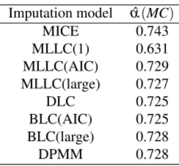
In order to see whether focusing on a single scale improves the estimate of Cronbach’s alpha, we performed a separate MI with MICE and the LC methods for the 30 items of the MC scale (the scale with the worst results in terms of ˆα, compared with the results of Table 2). From Table 5 it can be seen that MLLC(AIC), MLLC(large), DLC, BLC(AIC), BLC(large), and DPMM are doing much better now, their estimates being much closer to those of Table 2. MLLC(1), on the other hand, is still doing badly, which confirms that it is an inadequate imputation model. MICE produced a Cronbach’s alpha identical to the one with all 91 variables.

Table 5:Comparsion ofαˆ (MC scale) estimated after performing MI only on items of MC scale.

Imputation model αˆ(MC)

MICE 0.743

MLLC(1) 0.631

MLLC(AIC) 0.729

MLLC(large) 0.727

DLC 0.725

BLC(AIC) 0.725

BLC(large) 0.728

DPMM 0.728

Discussion

This paper offered a state-of-the-art overview on the use of LC models as tools for MI. One feature that makes LC models attractive imputation tools for psychological assessment studies is that they do not require complex model specification, since only the specification of the number of classes,K, is needed. Second, LC models can efficiently be computated even when dealing with a large number of variables. Third, by selecting a large enough number of classes, LC models can pick up complex associations in high-dimensional datasets.

Four possible LC implementation for MI were described: the Maximum Likelihood LC (MLLC), the Bayesian LC (BLC), the Divisive LC (DLC), and the Dirichlet Process Mixture of Multinomial Distributions (DPMM) approaches. While sharing the attractive features of LC modeling for MI, these methods differ in various ways. One is how they account for the uncertainty about the imputation model parameters: whereas MLLC

estimated model, the Bayesian methods (BLC and DPMM) draw parameters from their posterior distribution. Second, the decision regarding the number of classesKis handled differently by the four approaches. MLLC and BLC require model comparison through for example the AIC, DLC determinesKin a single run of its sequential algorithm, and DPMM leaves the number of classes unspecified. In MLLC and BLC, it is also possible

to setKto an arbitrary large value, which makes them more similar to DLC and DPMM,

also in terms of computation time.

We illustrated the use of the LC imputation methods and compared them with listwise deletion and MICE using a dataset with 91 categorical variables from a psychological assessment study. We looked at two situations: the original situation with a low rate of missingness and a situation with a much higher rate of missingness obtained by creating additional missing values. In the first situation, the various types of LC imputation models yielded very similar results; that is, similar Cronbach’s alpha values, means for men and women, standard errors and t-tests. However, the fact that the results obtained with the 1-class imputation model were also similar but those obtained with listwise deletion different indicated that in this low missingness case it was more important to keep the records with missing values than to have a correct imputation model. MICE imputation supplied estimates very similar to those of the LC models, although minor systematic differences appeared between these two different types of imputation methods.

The differences between LC imputation with both the under-specified model and MICE were much larger in the high missingness situation. The estimates for Cronbach’s alpha and the standard errors of the means were smaller (too small) in the 1-class model, showing that the imputation model matters. Furthermore, LC imputation methods introduced less bias in the estimates of means and standard errors than MICE in Case II, whereas MICE appeared to better recover the alpha for one scale but worse for the other four scales.

When comparing the LC-MI estimates of Cronbach’s alpha between the low and high missingness condition, we saw that alpha was underestimated with more missing values, where the degree of this underestimation varied per scale. This shows that also the LC-MI methods do not pick up perfectly the variability in and the associations between the variables in the dataset. When performing the imputation for a single subscale rather than for all 91 variables simultaneously, the LC MI models yielded much better estimates for Cronbach’s alpha. Capturing the associations among the variables turns out to be easier with a smaller more homogeneous set of items, showing that in practice it may be a good idea to perform the imputation per subset. Whether this is generally the case, is something that needs future research.

research. The first, and most important, is their moderate performance in capturing all the associations with high rates of missingness. It may be that we need an even larger number of classes than we used in our application. In the Bayesian specification, we have to specify the prior distributions for the parameters, and it is well known that the choice of priors may affect the results. Therefore, also the specification of the priors in the context of LC-MI needs further study.

Moreover, LC models can easily be extended with a regression model in which the latent classes are predicted using background variables, such as sex, age, and education level. Such an approach has not been used for MI yet, but it may be interesting to investigate whether inclusion of explanatory variables may improve the obtained imputations.

While we focused on the LC-based imputation methods for cross-sectional categorical data, the methods may also be applied with mixed categorical and continuous data, as well as with more complex longitudinal or multilevel designs. This reflects the wide range of applications in which LC models can be used. For instance, LC models for multilevel data (both for continuous and categorical variables) are described by Vermunt (2008), while latent Markov models for longitudinal data are among others described by Baum, Petrie, Soules, and Weiss (1970). Such more advanced LC models may also be used for MI. A possible Bayesian (DPMM) implementation of LC MI for longitudinal panel studies is provided by Si (2012).

References

Allison, P. D. (2009). Missing data. The SAGE Handbook of Quantitative Methods in

Psychology, 4, 72-89.

Baraldi, A. N., & Enders, C. K. (2010). An introduction to modern missing data analyses.

Journal of School Psychology, 48, 5-37.

Baum, L. E., Petrie, T., Soules, G., & Weiss, N. (1970). A maximization technique occurring in the statistical analysis of probabilistic functions of Markov chains.

Annals of Mathematical Statistics, 41, 164-171.

Brand, J. P. L. (1999). Development, implementation and evaluation of multiple

imputation strategies for the statistical analysis of incomplete data sets(Chapter 5). Dissertation. Erasmus University Rotterdam, The Netherlands.

Dempster, A. P., Laird, N. M., & Rubin, D. B. (1977). Maximum likelihood from

incomplete data via the EM algorithm. Journal of the Royal Statistical Society

Series B, 56, 1-38.

Diebolt, J., & Robert, C. (1994). Estimation of finite mixture distributions through Bayesian sampling. Journal of the Royal Statistical Society B, 56, 363-375.

Dunson, D. B., & Xing, C. (2009). Nonparametric Bayes modeling of multivariate categorical data.Journal of the American Statistical Association, 104, 1042-1051.

Efron, B. (1979). Bootstrap methods: another look at the Jakknife. The Annals of

Statistics, 7, 1-26.

Escobar, M. D., & West, M. (1995). Bayesian density estimation and inference using mixtures. Journal of the American Statistical Association,, 577-588.

Gebegziabher, M., & DeSantis, S. (2010). Latent class based multiple imputation ap-proach for missing categorical data. Journal of Statistical Planning and Inference, 140, 3252-3262.

Gelfand, A. E., & Smith, A. F. M. (1990). Sampling based approaches to calculating marginal densities. Journal of the American Statistical Association, 85, 398-409.

Geman, S., & Geman, D. (1984). Stochastic relaxation, Gibbs distributions, and the

Bayesian restoration of images. IEEE Transacations on Pattern Analysis and

Machine Intelligence, 6, 721-741.

Goodman, L. A. (1974). Exploratory latent structure analysis using both identifiable and unidentifiable models. Biometrika, 61, 215-231.

Graham, J. W., Olchowski, A. E., & Gilreath, T. D. (2007). How many imputations are really needed? Some practical clarifications of multiple imputation theory.

Prevention Science, 8, 206-213.

Graham, J. W., & Schafer, J. L. (1999). On the performance of multiple imputation for multivariate data with small sample size. In R. Hoyle (Ed.),Statistical strategies for small sample research, pp. 1-29. Thousand Oaks, CA: Sage.

Huisman, M. (1998).Item nonresponses: Occurrence, causes, and imputation of missing

answers to test items. Leiden, The Netherlands: DSWO Press.

Ishwaran, H., & James, L. F. (2001). Gibbs sampling for stick-breaking priors.Journal of the American Statistical Association, 96, 161-173.

Princeton University Press.

Linzer, D., & Lewis, J. (2014). poLCA: Polytomous variable Latent Class Analysis

[Computer software manual]. Retrieved fromhttp://cran.r-project.org/

web/packages/poLCA/index.html (R package version 1.4.1.)

Little, R. J. A., & Rubin, D. B. (2002).Statistical analysis with missing data(2nd ed.). New York: Wiley.

Liu, J. S. (1994). The collapsed Gibbs sampler in Bayesian computation with application to a gene-regulation problem.Journal of the American Statistical Association, 89, 958-966.

McLachlan, G. J., & Peel, D. (2000).Finite mixture models. New York: Wiley.

Roth, P. L. (1994). Missing data: A conceptual review for applied psychologysts.

Personnel Psychology, 47, 537-560.

Rubin, D. B. (1976). Inference and missing data.Biometrika, 63, 581-592.

Rubin, D. B. (1987).Multiple imputation for nonresponse in surveys. New York: Wiley.

Schafer, J. L. (1997). Analysis of incomplete multivariate data. London: Chapman & Hall.

Schafer, J. L., & Graham, J. W. (2002). Missing data: Our view of the state of the art.

Psychological methods, 7, 147-177.

Schlomer, G. L., Bauman, S., & Card, N. (2010). Best Practices for Missing Data

Management in Counseling Psychology. Journal of Counseling Psychology, 57,

1-10.

Sethuraman, J. (1994). A constructive definition of Dirichlet priors.Statistica Sinica, 4, 639-650.

Si, Y. (2012). Nonparametric Bayesian methods for Multiple Imputation of large scale

incomplete categirical data in panel studies. Ph.D. Thesis. Duke University, USA.

Si, Y., & Reiter, J. P. (2013). Nonparametric Bayesian Multiple Imputation for

In-complete Categorical Variables in Large-Scale Assessment Surveys.Journal of

Educational and Behavioral Statistics, 38, 499-521.

Tanner, A. M., & Wong, W. H. (1987). The calculation of posterior distributions by Data Augmentation.Journal of the American Statistical Association, 82, 528-540.

Van Buuren, S., Groothuis-Oudshoorn, K., Robitzsch, A., Vink, G., Doove, L., & Jolani, S. (2014). mice: Multivariate Imputation by Chained Equations [Computer

soft-ware manual]. Retrieved fromhttp://cran.r-project.org/web/packages/

mice/index.html (R package version 2.22)

Van Buuren, S., & Oudshoorn, C. (1999).Flexible multivariate imputation by MICE

(Tech. rep. TNO/VGZ/PG 99.054). Leiden: TNO Preventie en Gezondheid.

Van den Broek, K., Nyklicek, I., Van der Voort, P., Alings, M., & Denollet, J. (2008). Shocks, personality, and anxiety in patients with an implantable defibrillator.

Pacing Clin Electrophysiol., 38, 850-857.

Van der Palm, D. W., Van der Ark, L. A., & Vermunt, J. K. (2013a). A comparison of incomplete-data methods for categorical data.Statistical Methods in Medical Research.

Van der Palm, D. W., Van der Ark, L. A., & Vermunt, J. K. (2013b). Divisive latent

class modeling as a density estimation method for categorical data.Manuscript

submitted for publication.

Van der Palm, D. W., Van der Ark, L. A., & Vermunt, J. K. (2014). Divisive latent

class modeling as an incomplete-data method for categorical data. Manuscript

submitted for publication.

Van Ginkel, J. R. (2007). Multiple imputation for incomplete test, questionnaire and

survey data. Ph.D. Thesis. Tilburg University, The Netherlands.

Vermunt, J. K. (2008). Latent class and finite mixture models for multilevel datasets.

Statistical Methods in Medical Research, 17, 33-51.

Vermunt, J. K., & Magidson, J. (2013).LatentGOLD 5.0 Upgrage manual. Belmont,

MA: Statistical Innovations Inc.

Vermunt, J. K., Van Ginkel, J. R., Van der Ark, L. A., & Sijtsma, K. (2008). Multiple imputation of incomplete categorical data using latent class analysis.Sociological Methodology, 38, 369-397.

White, A., & Murphy, B. (2014). BayesLCA: Bayesian Latent Class Analysis

[Com-puter software manual]. Retrieved fromhttp://cran.r-project.org/web/

packages/BayesLCA/index.html (R package version 1.5)

Wilkinson, L., & Task Force on Statistical Inference. (1999). Statistical methods in

psychology journals: Guidelines and explanations. American Psychologist, 54,

Appendices

Bayesian Tools

The Dirichlet Distribution

In Appendices A and B, f(·)will denote a generic probability distribution or density. The Dirichlet Distribution will be denoted with Dir(λ), where λ = (λ1, ...,λd)is a multi-dimensional parameter.

Suppose we have a random variableU with d components (d ≥2) such thatU =

(U1, ...,Ud); thenU∼Dir(λ), or equivantly,

f(U|λ) = 1

B(λ) d

∏

i=1

udi−1

i

in thed-dimensional simplex{(u1, ...,ud):ui∈R+∀i,u1+...+ud=1}. Here, each

ui is a realization ofUiandB(λ)is the multivariate Beta function. Whend=2, the Dirichlet distribution becomes a Beta distribution.

This density can be used to model sets of probabilities of mutually exclusive and exhaustive events. This property, as well as its functional form, makes the Dirichlet distribution a conjugate candidate for the Multinomial distribution, thus forming the Dirichlet-Multinomial conjugate. According to this model, if the prior distribution of the set of parameters of the Multinomial distribution withdcategories, sayπ, follows a Dirichlet distribution with parameterλ = (λ1, ...,λd)and the dataY= (Y1, ...,Yd)are

assumed to be distributed according to a Multinomial distribution withdcomponents,

then the resulting posterior is λ|Y ∼Dir(λ1+Y1, ...,λd+Yd). In case ofd=2 the Dirichlet-Multinomial conjugate corresponds to the Beta-Binomial.

Bayesian Computation

The Gibbs sampler

Consider a L-dimensional random variableθ= (θ1, ...,θL)and suppose that we want to compute the marginal densities f(θi),i=1, ...,L. Furthermore, suppose that these marginal densities are obtainable by integration, f(θi) = f(θ1, ...,θL)d(θ−i), in which

but that a series of conditional distributions f(θi|θ−i)is available for eachi=1, ...,L.

The Gibbs sampler, after initializing the variables with some valueθ(0)_{= (θ}(0) 1 , ...,θ

(0) L ), proceeds as follows:

1. Drawθ₁(t+1)∼f(θ1|θ2(t), ...,θ (t) L )

2. Drawθ₂(t+1)∼f(θ2|θ1(t+1),θ (t) 3 ...,θ

(t) L ) ..

.

L. Drawθ_L(t+1)∼f(θL|θ1(t+1),θ (t+1) 2 ...,θ

(t+1) L−1 )

fort=1, ...,T, whereT is the total number of iterations of the sampler. Under mild conditions, the Gibbs sampler converges to the stationary distributions f(·). For further technical details, we refer to Gelfand and Smith (1990). Liu (1994) argued that the efficiency of the Gibbs sampler can be further improved by considering blocks of correlated components together. For instance, it is possible to groupθinto two blocks,

G1= (θ1, ...,θ_d′)andG₂= (θ

d′+1, ...,θL). The result is a two-blocks Gibbs sampler:

1. DrawG(₁t+1)∼f(G1|G(2t))

2. DrawG(₂t+1)∼f(G2|G(₁t+1))

fort=1, ...,T.

The Data Augmentation Algorithm

The Data Augmentation (DA) Algorithm (Tanner & Wong, 1987) is a special case of the Gibbs sampler. It exploits the fact that

f(θ|Y) =

Z

h(θ,Z|Y)dz,

that is, thecompletionordata augmentationof f. Here,Z are unobserved or latent

data whose support is denoted byZ_{, whereasY denotes a set of observed variables and}

h(·)is a probability density function. The aim of the DA algorithm is to simplify the sampling from the joint distribution f(θ|Y)through a simpler conditional distribution

f(θ|Z,Y). For the DA algorithm, both f(θ|Z,Y)and f(Z|θ,Y)must be available. After initializing the unobservedZand the values ofθ with some arbitrary valuesZ(0) and

θ(0)_{, the algorithm consist of two steps:}

– Posterior Step: Drawθ(t+1)_∼f(θ|Y,Z(t+1)₎

fort=1, ...,T. In fact, this a version of the DA algorithm in which a singleZ-value is drawn at each step. The original DA algorithm with multipleZ-value draws, as well as the conditions for convergence to the target distribution, can be found in Tanner and Wong (1987).

The DA algorithm can be seen as the Bayesian counterpart of the EM algorithm. Since both latent variables and missing data can be treated as unobserved values, this algorithm is of particular interest in applications such as LC-MI.

Bayesian Multiple Imputation via Mixture Modeling

The notation and the model specification are the same as described in Section 2.1. The parameters of a specific classk (i.e.,πππyyyjjj whenx=k) will be denoted by πππ

kkk jjj. For parameters initialization and implementation of the algorithms, we follow Si and Reiter (2013). In order to simplify notation, a dot in the condition sign, i.e.P(|·), will indicate a conditioning on all the data and other parameters included in the model.

The Bayesian Latent Class Multiple Imputation Model

a. Distributional assumptions. -Data likelihoods:

– xi∼Multinom(πππxxx) where Multinom(πππxxx) is the Multinomial distribution with parame-terπππxxx= (π1, ...,πk, ...,πK)∀i;

– Yi j|xi=k∼Multinom(πππkkk_jjj)))withπππkkk_jjj= (πkj1, ...,πkjd, ...,πkjdj)wheredjis the number

of categories of the variableYj∀i,j.

-Parameters priors:

– πππxxx∼Dir(αααxxx)withαααxxx= (α1, ...,αk, ...,αK);

– πππkkk

jjj∼Dir(αααkkkjjj)withαααkkkjjj= (αkj1, ...,αkjd, ...,αkjdj).

b. Implementation. -Parameters initialization:

– setααα(xxx0)= (α1(0), ...,α (0) k , ...,α

(0)

K ) = (1, ...,1);

– setαααkkk_jjj(0)= (α_j1k(0), ...,αk_jd(0), ...,αk_jd(0)

– initializeπππ(xxx0)with a draw from the Dirichlet distribution with parametersααα( 0) xxx

– setP(yi j=d|xi=k;πππyj)

(0)_=πk(0)

jd =fˆ(yj,obs=d)∀i,j,k, where ˆf(yj,obs=d)is the

marginal observed empirical probability thatyi j=d;

– sample a value forYi j,misfrom ˆf(yj,obs) ∀iinYj,mis.

-The algorithm: Fort=1, ...,T:

1. samplex(_it)∈ {1, ...,K} ∀i=1, ...,nfrom a Multinomial distribution withposterior membership probabilitiesas parameters:

P(x(_it)=k|·) =

π_k(t−1)∏J_j=1

∏d_d=j ₁πk_jd(t−1)

I_{(yi j=d)}

∑_hK₌₁π_h(t−1)∏J_j=1

∏d_d=j ₁πh_jd(t−1)

I_{(yi j=d)}

whereI_{(yi j=d) =1 ifyi j=dand 0 otherwise;}

2. sample

(πππ(xxxt)|·)∼Dir

α₁(0)+

n

∑

i=1 I_(x(t)

i =1), ...,α (0)

K +

n

∑

i=1 I_(x(t)

i =K)

where I_(x(t)

i =k)is an indicator variable which is equal to 1 if x

(t)

i =kand 0

otherwise;

3. draw

(πππk_j(t)|·)∼Dir ⎛

⎜ ⎝α

k(0)

j1 +

∑

i:x(_it)=k

I_{(yi j=1), ...,α}k(0)

jdj +

∑

i:x(_it)=k

I_{(yi j=dj)}

⎞

⎟ ⎠

∀i,j,k;

4. (imputation step): given the valuex(_it)=kof each unit, for each{i,j}inYmissample

from

(Y_{i j}(t)|·)∼Multinom(πππk_j(t)).

Once the MCMC chain has completed its iterations, themimputations are obtained by