Comparing Macroeconomic Returns on Human and Public Capital:
An Empirical Analysis of the Portuguese Case (1960-2001)
June 2004
Álvaro Manuel Pina, [email protected] Miguel St. Aubyn, [email protected]
ISEG and UECE
Instituto Superior de Economia e Gestão Technical University of Lisbon
R. Miguel Lupi, 20 P-1249-078 Lisbon, Portugal
Álvaro Manuel Pina, [email protected] Miguel St. Aubyn, [email protected] ISEG and UECE
Instituto Superior de Economia e Gestão Technical University of Lisbon
R. Miguel Lupi, 20, P-1249-078 Lisbon, Portugal JEL codes: I20, H54, O47
Keywords: Human capital, public capital, economic growth, Portugal.
Abstract:
The impact of human and public capital on growth is a major issue in economic theory and in policy evaluation. Using a cointegrated VAR, we estimate a Cobb-Douglas production function for Portugal with public and human capital. Return rates are then computed with and without dynamic feedbacks. Without these, human capital yields a return comparable to private investment, and smaller than public investment. Considering dynamic feedbacks, private capital responds positively to a shock in public capital, but negatively to a shock in human capital. Consequently, the dynamic feedbacks return on human capital is much lower than on public capital.
Policies to promote growth, in the European Union (EU) and elsewhere, are usually based on the belief that human capital formation and public investment have a long-lasting effect on aggregate production. In the EU, less developed economies have been on the receiving end of structural funding in order to foster real convergence, meaning an approximation to richer countries income levels. Recipient economies have included Greece, Ireland, Italy, Spain, Portugal and several regions of other countries. Also, all ten countries that entered the EU in May 2004 will be beneficiaries of this European regional policy. Community funds directed to converging economies co-finance an important number of government programs in what concerns public investment (roads, railways, airports and ports, schools and hospitals and other public infrastructure) and also human capital formation, in both the formal education system and training. It becomes therefore essential, from a policy evaluation point of view, to have a quantified measure of the impact of both human capital and public investment on the growth performance of receiving economies.
A second motivation for this paper stems from the current debate on fiscal rules in Europe, especially as regards the treatment of public investment. Some economists argue that this kind of spending is discouraged under the rules of the Stability and Growth Pact (SGP), and that public investment should therefore be excluded from the deficit definition to which ceilings apply. Blanchard and Giavazzi (2004), for instance, propose a golden rule applying to net public investment. Critics of the golden rule, among other arguments, point out its vulnerability to creative accounting, warn that a preferential treatment of physical investment could bias expenditure decisions against spending on education and R&D, and stress that what matters is the overall capital stock, be it private or public (see e.g. Buti, Eijffinger and Franco, 2003). Against this background, it is clearly important to assess how “productive” public capital really is, especially by comparison with private capital and human capital. It is also relevant to study the impact of public investment on the overall (physical) capital stock. In the light of the above motivations, this paper computes rates of return on public capital and on human capital for the Portuguese economy, using a new data set with annual data (from 1960 to 2001) on GDP and four production factors: labor, private (physical) capital, public capital and human capital. Most inputs for deriving such rates follow from the estimation of a cointegrated vector autoregression (VAR), where the cointegrating vector can be interpreted
as an aggregate four-factor Cobb-Douglas production function. While this vector forms the basis to compute returns on a given factor holding all the others constant (which we term the ceteris paribus rate of return), the estimated VAR also allows us to consider the dynamic responses of all the variables in the system to a structural shock to public or human capital, giving rise to what we call the dynamic feedbacks rate of return.
From a methodological point of view, our work contains two main innovative features. First and foremost, we study the importance of public capital and human capital in a unified, coherent framework, rather than separately, as is common in the literature. In this way we are in a position to compute rates of return on each of those two inputs which are comparable and which control for the contribution of the other input. Second, we consider alternative definitions of rates of return, clarifying the underlying assumptions. Again, this enables us to compare magnitudes that previous studies had computed in isolation.
The issues motivating this study concern a wide range of countries, to which our methodology would also be applicable. The empirical focus on Portugal was mainly dictated by reasons of data availability for human capital: Pereira (2003) provides a carefully constructed annual series for the average years of schooling of the Portuguese adult population, something which is not available (with annual periodicity) for most other economies. Care has also been taken to ensure that our measures of private and public capital reflect the best available statistical information.
The remainder of this study is organized as follows. Section 2 surveys the literature on the contribution of public capital and human capital to economic growth. In section 3 we present the production function to be estimated, and discuss in detail the computation of rates of return under alternative assumptions. Our data set is described in section 4, with an emphasis on the construction of physical capital stocks, as well as on the chosen proxy for human capital. Section 5 contains the empirical results regarding the specification and estimation of a cointegrated VAR and the ensuing rates of return on public and human capital. Section 6 concludes.
2. Literature overview
Public capital and growth
In the economic literature, it is not taken for granted that public investment has a significant impact on growth1. The works of Aschauer (1989a, 1989b, 1990) on the US economy suggested that the elasticity of output with respect to the public capital stock was about 0.39, and that returns to public investment were higher than returns to private investment. These results were supportive of a particular explanation of the productivity slowdown felt at the time – that it was due to a decline in public investment. Aschauer’s findings were criticized on several methodological grounds, and these critiques have led to the application of different econometric techniques to the public capital issue. At the same time, several studies were made to other countries than the US.
Aschauer results relied on static OLS regressions performed with series that are not usually stationary. As it is now well understood, least squares regression may lead to spurious results if there is no cointegration among the variables. Tatom (1991) showed that using first differences led to a much smaller and statistically insignificant effect of public investment on growth. Also, the estimation of a static equation is not immune to the reverse causality problem – public capital may well be caused by output, and not the contrary. Aaron (1990) first made this point.
Subsequent researchers have taken these points seriously. VAR analysis has become a more usual tool, as it allows for the endogeneity of both production and public capital and for dynamic effects between the variables. The finding that series are cointegrated has made some researchers consider a cointegrated VAR, or a VAR with an error-correction mechanism. Crowder and Himarios (1997), Lau and Sin (1997) and Pereira (2000) applied VAR analysis to the US case. In a similar vein, Batina (1999) deals with cointegration and dynamic causality issues by resorting to dynamic ordinary least squares (DOLS). Recent studies that follow a VAR approach applied to European countries include Flores de Frutos, Gracia-Díez and Pérez-Amaral (1998) and Pereira and Roca (2001, 2003) for Spain, Evareart (2003) for Belgium, and Ligthart (2000) and Pereira and Andraz (2002, 2004) for Portugal. In general terms, Batina’s (2001) inferences from the empirical literature – that public capital
1Surveys on the "public capital hypothesis" include Batina (2001), Congressional Budget Office (1998),
has a positive but not tremendous effect on economic growth, that some types of public investment have more impact than others, and that, in statistical terms, it is perfectly possible to find little or no effect of public investment, "even after careful statistical work has been done" (p. 125) – seem an adequate synthesis2.
Results specific to the Portuguese economy do not abound. Ligthart (2000) estimates a production function associated to a cointegrating vector in a VAR. The estimated public capital elasticity of output is high, between 0.37 and 0.39, and close to the US value estimated by Aschauer (1989a, 1989b). The same author reports results from an unrestricted VAR analysis that confirm public capital as a significant long-term determinant of output growth, and a disaggregation showing that transport infrastructures are more productive than other types of public investment. Pereira and Andraz (2002) analyze the effects of public investment in transportation infrastructures on Portuguese economic performance. Using a VAR methodology, they find important positive long run effects of aggregate public investment on production, employment and private investment. The rate of return to public investment is close to 16%. Their data set allows them to perform a discrimination of these effects by types of investment. In Pereira and Andraz (2004), they present results in more detail together with sectoral and regional disaggregations.
Human capital and growth
Country-specific studies concerning human capital and growth are scarce, probably because human capital data is seldom available on an annual basis. Consequently, effects on growth have often been estimated by resorting to cross-sectional regressions3. The dependent variable is usually GDP, either in levels or in growth rate terms, sometimes divided by population or by the number of workers. A proxy for "human capital" is included among the explanatory variables. The most common proxies are school enrolment rates and the average number of schooling years, or other variables closely related to the educational attainment of the adult population.
2 Another line of applied research in this field follows a cost function minimisation approach. As we do not
pursue this approach, we refer the interested reader to Batina (2001) and to Pereira and Andraz (2004) for an exposition and references.
3 Krueger and Lindahl (2001) Sianesi and Van Reenen (2002) and De la Fuente and Ciccone (2002) survey the
Specification options strongly condition empirical results. As emphasized by De la Fuente and Ciccone (2002) and Sianesi and Van Reenen (2002), there is a dichotomy between a levels and a growth rate specification. In the former, human capital affects the level of GDP per head, or productivity. This type of specification is usually associated to an augmented neo-classical growth model, like the one proposed by Mankiw, Romer and Weil (1992). In a growth rate specification, the human capital stock affects changes in GDP per head or productivity. This latter option is usually related to "new" or "endogenous" growth models4. When a growth rate specification is adopted, the impact of human capital investment is potentially greater, especially in a long run perspective.
Several studies find that there is a significant and positive relationship between human capital and growth. Nevertheless, there remains considerable uncertainty concerning the magnitudes involved. De la Fuente (2003), who follows a production function approach comparable to ours, uses a parameter range for his human capital elasticity based on a literature survey and on own estimates. According to this author, and considering EU countries, a 1 percent increase in average years of schooling implies a percentage increase in the GDP level between 0.394 and 0.587.
In what concerns Portugal, Teixeira (1996), Teixeira and Fortuna (2003) and Pina and St. Aubyn (2002) were the sole country-specific studies known to us that provide estimates of the human capital contribution to economic growth. Teixeira and Fortuna obtain a GDP level elasticity with respect to human capital (measured as average years of schooling) close to 0.42. Pina and St. Aubyn estimates are similar – between 0.36 and 0.48.
3. The aggregate production function and the returns to investment
To study in a common framework the importance of human capital and public capital for Portuguese economic growth, we specify a Cobb-Douglas production function,
[
]
γ(
)
α β −α−β = exp( ( )) ( ) ( ( )) ( )1 ) (t A H t KP t KG t L t Y , (1)4 For example, in Lucas (1988) model of learning by studying, the output growth rate is closely related to the
where Y is GDP, KP is the private capital stock, KG is the public capital stock (all in real terms), H is our measure of human capital (average years of schooling), L denotes employment and A is a constant scale parameter. All variables will be defined in detail in section 4.
Dividing by and taking logs in equation (1), the production function can be written in condensed form: ) (t L ) ( ) ( ) ( ) (t c H t kp t kg t y = +γ +α +β , (2)
where a lower case variable denotes values per worker (i.e., divided by L) in log terms.
We impose constant returns to scale across physical capital (both private and public) and labor, but leaving out human capital. Many other studies have made a similar assumption5, which can be justified on grounds of a standard replication argument6. One should also notice that, due to the way human capital enters the production function, parameter γ is a semi-elasticity, indicating the percentage increase in output that would result from one more year of schooling for the average worker. This formulation is reminiscent of the well-known Mincerian wage equations (percentage increase in wages due to one more year of schooling), and has been previously adopted in some macroeconomic studies as well (e.g. Jones, 2002).
Both for investment in public capital and in human capital, we compute rates of return (r.o.r.) in two different ways, which we call the “ceteris paribus r.o.r.” and the “dynamic feedbacks r.o.r.”. Each will be now presented and discussed, starting with the case of public capital. Public capital rates of return
The ceteris paribus r.o.r. corresponds to the usual definition of a rate of return, based on the discounted value of the stream of increases in output due to a unit investment in the present (time 0), holding all other inputs constant. Formally, this r.o.r. is the value of r that solves the equation
5 See, for example, De la Fuente (2003), De la Fuente and Doménech (2000), Cohen and Soto (2001), Everaert
(2003) and Teixeira and Fortuna (2003).
6 Doubling the physical capital stocks and the number of workers, and keeping unchanged the average level of
1 )) ( / ) ( (
∫
∞ − − = ∂ ∂ o rt te dt e t KG t Y δ , (3)where the marginal productivity is computed on the basis of the production function, and the rate of depreciation δ takes account of the fact that the initial unit increase in the stock of public capital will gradually fade away.
Using the production function elasticity β, one can write , and assuming, as an approximation, that the capital/output ratio stays constant
)) ( / ) ( ( ) ( / ) (t KG t Y t KG t Y ∂ =β ∂
7, the r.o.r. becomes
δ β − = KG Y r . (4)
The dynamic feedbacks r.o.r. drops the ceteris paribus assumption, and considers how the other inputs respond to an increase in public capital. Such a response is an important factor to be taken on board when assessing the merits of public investment, particularly as regards whether public capital crowds in or out private capital. VAR models provide the standard framework to quantify the dynamic responses of several variables to a (structural) shock in one of them; hence, following Pereira (2000) and Pereira and Andraz (2002, 2004), our dynamic feedbacks r.o.r. draws on the impulse response functions (IRFs) of a VAR model with output and the several inputs.
Formally, we compute the value of r that solves the equation
∫
∫
∞ − ∞ − = o rt b o rt bY t e dt d IG t e dt d ( ) ( ) , (5)where IG denotes public investment and db stands for the differences relative to baseline, given by the IRFs8.
7 This will hold in a steady state, and can be regarded as an acceptable simplification even in the case of
catching-up economies, where the Y/KG ratio has not displayed a clear-cut trend (see section 4 and Kamps, 2003).
8 By “baseline” we mean a scenario where no shock to public investment would occur. While deferring to
section 5 the details on the computation of dbY and dbIG, we add at this point that equation (5) differs from
Pereira (2000) and Pereira and Andraz (2002, 2004), since they only consider the long-term values of dbY and
The only difference between equations (3) and (5) lies in the way of calculating the increases in output and public investment9, which in turn hinges upon whether the ceteris paribus assumption is appropriate. Pereira (2000) strongly defends that induced changes in private inputs should be taken into account, and that the ensuing “total marginal product” of public investment (dbY/dbIG, in our notation) is “the relevant concept from the standpoint of policy-making” (ibid., p. 517). While agreeing that dynamic feedbacks are of indisputable relevance, our view is that there are valid arguments both for and against their inclusion into the r.o.r.. Against the dynamic feedbacks r.o.r., one may point out that if private investment is crowded in (out), its cost should be included in (deducted from) the right-hand side of equation (5), rather than ignored, as is the case. On the other hand, the output effects of such crowding in (or out) should be, to some extent, credited to public investment, as they would not take place in its absence – a shortcoming of the ceteris paribus r.o.r.. Taking an agnostic approach, we will compute both rates of return10.
Human capital rates of return
Again, we start with the ceteris paribus r.o.r.. We assume that human capital formation falls on the young, and consider the macroeconomic costs and benefits stemming from the decision of a 16-year-old to stay one more year at school, instead of joining the workforce.
The literature (e.g. De la Fuente, 2003) considers two main costs of schooling – the opportunity cost of studying and the direct costs of education (mainly teachers’ wages). Instead of trying to quantify these costs in money terms through off-model computations, we measure them by the marginal productivity of labor, derived from the production function. If a 16-year-old attends school for one more year, the total labor costs involved are equal to:
) 1 ( ) 1 ( −us + −ut = τ µ , (6)
where us is the unemployment rate for 16-year-olds, τ is the teacher/student ratio and ut is the
unemployment rate for teachers. Equation (6) takes into account that some students or
9 Notice that(∂Y(t)/∂KG(t))e−δtdKG(0), with dKG(0) = 1, is the counterpart of dbY(t).
10 There are cases where we have stronger beliefs: for instance, to assess whether public investment “pays for
itself” (by generating fiscal revenues), dynamic feedbacks should definitely be taken into account (see Pereira, 2000, p. 517).
teachers would be otherwise unemployed, schooling entailing in their case no loss of labor for other activities.
Total costs in terms of output are therefore equal to:
) 0 ( ) 0 ( ) 1 ( ) 0 ( ) 0 ( L Y L Y µ α β µ = − − ∂ ∂ , (7)
assuming that investment in human capital takes place at time 0.
As for benefits, we simply consider the present value of output gains brought about by the increase in H. In De la Fuente (2003), other benefits are taken into account, such as a decrease in the probability of unemployment (i.e., the unemployment rate) or a technological catch-up effect. The latter requires that at least a second country (the technological leader) is included in the analysis, which is not the case in this paper. As for the former, we decided to keep the unemployment rate independent from H: while at a microeconomic level a more educated individual may find it easier to get a job (indeed, De la Fuente documents that, in virtually every country, better educated workers have higher probabilities of employment - ibid., p. 60), at a macroeconomic level there is scant evidence that an increase in the average level of schooling lowers the natural rate of unemployment.
Benefits are therefore equal to:
∫
∞ − ∂ ∂ 0 ) ( ) ( ) ( dt e t dH t H t Y rt , (8) where ) ( 1 ) ( t POP t dH = and ( ) ) ( ) ( t Y t H t Y =γ ∂ ∂. POP(t) is the population aged 15 to 64. Since a youngster has a full working life ahead of him or her, equation (8) ignores any depreciation of the human capital formation (i.e., it is ignored that the 16-year-old will eventually retire). If we assume that population is constant and that output grows at a constant annual rate, g, the ceteris paribus r. o. r. is the value of r that solves the following equation:
) 0 ( ) 0 ( ) 1 ( ) 0 ( ) 0 ( 1 0 ) ( L Y dt e Y POP t r g µ α β γ = − −
∫
∞ − . (9) One obtains: ) 0 ( ) 1 ( ) 0 ( POP L g r β α µ γ − − + = . (10)The rate of return in equation (10) depends on three production function parameters (elasticities or semi-elasticities of inputs, to be estimated), and also on , L(0) and POP(0). Using values from Table 1, it becomes possible to express the human capital ceteris paribus r.o.r. as a function of production function parameters only:
µ β α γ − − + = 1 648 . 0 035 . 0 r . (11) Table 1
Parameter values used to compute the human capital ceteris paribus r.o.r.
Parameter Value Description Source
s
u 0.051 Unemployment rate of the population aged 15-19 not having completed upper
secondary education, 2001
OECD (2003), p. 297.
t
u 0.05 Unemployment rate, Eurostat definition, 2001
AMECO database11, May 2004.
τ 0.125 Ratio teachers/students, upper secondary, 2001.
OECD (2003), p. 330.
µ 1.06775 Labor costs (equation (6)) (1 ) (1 )
t s u u + − − = τ ) 0 (
POP 7 006 022 Population aged 15-64, 2001. Pereira (2003) )
0 (
L 4 848 412 Civilian employment, persons, 2001 AMECO database, May 2004
g 0.035 Output per employed person average growth rate, 1961-2001
AMECO database, May 2004
11 AMECO - Annual Macro Economic Database, European Commission. Available online at:
The dynamic feedbacks r.o.r. of human capital formation is computed in a similar way to its counterpart for public investment. It is the value of r that solves the equation
∫
∫
∞ − ∞ − = o rt b o rt bY t e dt d IH t e dt d ( ) ( ) , (12)where IH denotes investment in human capital. As in equation (5), db denotes differences
relative to baseline, inferred from the IRFs. Investment in human capital is recovered from changes in the stock of human capital (H), and expressed in real euro terms using equation (7).
4. Data
Physical capital
To construct a measure of physical capital (either private or public), one needs two basic ingredients: a time series of gross fixed capital formation (GFCF) flows, and a method for cumulating them into stocks. As regards the latter, we follow Kamps (2003), who has recently computed capital stocks for several OECD countries. However, instead of drawing on OECD investment data, as Kamps does, we resort to national sources, which we deem more accurate. Our main source is Banco de Portugal (1997), where an effort was made to remove breaks in series by recalculating older values in the light of more recent statistical concepts and methodologies. Several investment series are provided, from 1953 to 199512. From 1995 onwards we have used ESA 95 data provided by Instituto Nacional de Estatística, removing discontinuities in the common year (1995) by applying backwards the growth rates of the Banco de Portugal series to the ESA 95 levels13. Our GFCF series, therefore, cover the period 1953-2001.
12 Available on-line at www.bportugal.pt.
13 Admittedly, this is a shortcut, though of very common use. The ideal solution would be to reconstruct the
We have computed investment series at constant 1995 prices for the whole economy and for the public sector (general government)14, obtaining private investment by difference. As regards the whole economy, the above sources provide data with and without housing. We have chosen to include it, for two reasons: first, for consistency, since no GFCF series net of housing could be computed for the general government; second, because residential assets themselves generate value added (branch 70 in ESA 95), which is included in GDP15.
Having constructed investment series, we calculate stocks by the perpetual inventory method with geometric depreciation. The law of motion for a given capital stock, either private or public, can be written as
1 1 1 1 ) 2 1 ( ) 1 ( − − − − + − − = t t t t t K I K δ δ , (13)
where Kt is the beginning-of-period stock, It is the corresponding GFCF variable (again, either
private or public), and δt is a time-varying depreciation rate.
As in Kamps (2003), the rates of depreciation for non-residential assets remain constant until 1960, and then gradually increase over time16, according to
(
)
(
/ 1/41)
1960 , 1960,...,2001 1960 2001 1960 = = t− t t δ δ δ δ . (14)For public capital, the values of δ1960 = 0.025 and δ2001 = 0.04 are assumed, while for private
capital we posit δ1960 = 0.0275 and δ2001 = 0.0717.
14 In Banco de Portugal (1997) data for general government GFCF is only reported in nominal terms. However,
it includes a breakdown by types of capital goods (e.g. vehicles, construction, etc), and applying to each of these the corresponding price index (computed for the whole economy) has enabled us to produce estimates of public investment at constant prices.
15 Kamps (2003) estimates the residential capital stock separately for several countries in his sample, but not for
Portugal.
16 Using data from the Bureau of Economic Analysis, Kamps (2003) shows that the implicit scrapping rates in
the USA display an upward trend. Though similar data is not available for the Portuguese economy, it is worth mentioning that the depreciation rates accepted by the tax authorities for different types of assets generally increased from 1981 to 1990 (Decreto Regulamentar no. 2/90 versus Portaria no. 737/81).
17 These rates for private capital are slightly below those of Kamps, since he considers residential assets (which
To generate initial values for the capital stock, and again following Kamps (2003), artificial GFCF series starting in 1860 were constructed by assuming 4% real annual growth from that year to the start of our actual investment series (1953).The capital stocks in 1860 were then initialized at zero, and equation (13) run until 2001.
Human capital
We have used Pereira’s (2003) series for the average years of schooling of the Portuguese population aged between 15 and 64, a range close to the working force. The author anchored his series in census data and computed figures for years between censuses using data from different national sources on school enrollment, migration, mortality rates and retiring population. The use of interpolations or estimations was kept to a minimum.
It should be emphasized that the human capital series used in this paper is an annual one. Annual series on average years of schooling are not usually found in the empirical literature. However, they are essential for a time series, country-specific study like this one. Researchers on human capital and growth have mostly used series available at a five or ten year frequency, like the ones provided by Barro and Lee (2000), Cohen and Soto (2001) or De la Fuente and Doménech (2000). These data sets are interesting for panel data studies, with different countries as units of observation, but insufficient for use in a VAR.
GDP and employment
Our GDP and employment data come from the AMECO database, updated in May 2004. GDP is the gross domestic product at 1995 market prices and employment is civilian domestic employment.
The time series used in our empirical work are presented in the appendix and plotted in Figures 1 to 4. GDP per worker (Figure 1) grew faster from 1960 to 1974. Growth was somewhat disrupted following the first oil crisis and the democratic revolution in the middle of the 70s. Economic growth was reinforced after Portuguese accession to the European Community in 1986. Human capital, or average years of schooling, grew steadily from a very low value in 1960, less than 3 years, to a still low value in European terms in 2001 – a bit more than 7 years (see Figure 2). Public capital (Figure 3) tended to increase along GDP per worker. Public investment was particularly strong in recent years, in part due to structural funds made available by the EU. Private capital per worker, like GDP, grew at a higher rate in
the first part of the sample (Figure 4). The capital–output ratios displayed no clear trend, even if there was a jump in private capital relative to output in the mid 70s (Figure 5).
5. Empirical results18
The graphical analysis of the previous section suggests that all the series entering the production function (2) – GDP per worker, on the one hand, and the three capital inputs, also defined in per worker terms, on the other hand – are not stationary. If their first differences are stationary, then they can all be treated as I(1) series. In this case, there is the possibility that there is at least one linear combination of these four variables that is stationary. If there were a meaningful production function that links inputs to output then one would indeed expect to find such a stationary vector. The vector coefficients, if correctly normalized, would give us the elasticities we are interested in.
Accordingly, our empirical results are presented in the following sequence. Firstly, we show some evidence that the series are I(1). Secondly, we proceed to estimate the number, if any, of cointegrating vectors. Thirdly, once the number of cointegrating vectors has been chosen, we estimate a cointegrated VAR, yielding the parameters of the cointegrating vector(s) and the implied ceteris paribus r.o.r. Finally, drawing on the IRFs to structural shocks in human or public capital, we proceed to compute the dynamic feedbacks r.o.r..
Stationarity tests
Table 2 presents results from Augmented Dickey-Fuller (ADF) tests19. The first half of the table contains results when a trend was included in the regression. In the second half, no trend was included. The number of dependent variable lags was chosen starting from a relatively high value, nine lags, and sequentially reducing it when the t-statistic associated to the highest lag coefficient was not significant20.
18 Econometric results presented in this section were obtained using GiveWin and PcGive 10. See Doornik and
Hendry (2000, 2001) for a complete description of this software.
19 Augmented Dickey-Fuller tests are described in detail in several manuals of econometrics. See, for example,
Hayashi (2000).
20 The chosen maximum number of lags results from the formula proposed by Shwert (1989): = 4 1 100 12 T
Table 2
Augmented Dickey-Fuller tests Series in levels
Variable Lags included
ADF statistic Critical level 5% Critical level 1% Trend and constant included in the regression:
H 8 -2.177 -3.551 -4.260
kg 1 -3.161 -3.525 -4.202
kp 1 -1.250 -3.525 -4.202
y 8 -2.370 -3.551 -4.260 Constant but no trend included in the regression:
H 8 1.579 -2.953 -3.642
kg 0 -1.183 -2.934 -3.597
kp 1 -2.605 -2.936 -3.602
y 8 -1.196 -2.953 -3.642
The null hypothesis of no stationarity is not rejected in any case, as the ADF statistic is never inferior to the 5 percent critical level.
When the series are first differenced, the no stationarity hypothesis is dismissed in almost all cases, as can be inferred from Table 3. The number of lags was determined as above, and only a constant was included in the regression.
Table 3
Augmented Dickey-Fuller tests Series in first differences
Variable Lags included
ADF (or DF) statistic
Critical level 5% Critical level 1%
DH 1 -2.191 -2.938 -3.607
Dkg 0 -4.671** -2.936 -3.602
Dkp 0 -3.035* -2.936 -3.602
Dy 1 -3.990** -2.938 -3.607
* Rejection at the 5 percent level. ** Rejection at the 1 percent level.
The ADF test for the first difference of the human capital series was not conclusive in dismissing the non-stationarity hypothesis. This could well result from the fact that our sample is relatively small – it is well known that stationarity tests are not very powerful in small samples. In conceptual terms, it is difficult to believe that changes in average years of schooling have random walk properties. These changes result from higher schooling rates in younger cohorts. These schooling rates have clearly increased in Portugal from 1960 onwards, as they were very far from the 100 percent limit. As this limit is gradually approached, it is to be expected that changes in years of schooling become smaller. Visual inspection of Figure 2 suggests this could already be the case for Portugal from 1993 onwards. Accordingly, we take the H series as being I(1), the same order of integration as kg, kp and y.
Number of cointegrating vectors
In determining the number of cointegrating vectors, we followed the Johansen (1988) procedure. We started by estimating the following unrestricted VAR:
t p i i t i t t t c D X X X = +Φ + Γ∆ +Π +ε ∆
∑
=1 − −1 , (15)where Xt is a vector of four endogenous variables (kg, kp, H and y). This VAR includes an
unrestricted constant, c, which allows for linear growth in the data. Two unrestricted dummy variables, D1t, taking value 1 from 1960 to 1974 and equaling 0 from 1975 onwards, and D2t,
which equals 1 from 1986 onwards, and zero otherwise, were also included. The first artificial variable takes into account the structural break in growth that occurred in the mid-seventies, while D2t corresponds to the growth resurgence following Portuguese entry to the European
Community in 1986. The number of lags in the VAR, p , was chosen to be equal to 1, considering a residuals normality test and three information criteria (Schwarz, Hanann-Quinn and Akaike)21.
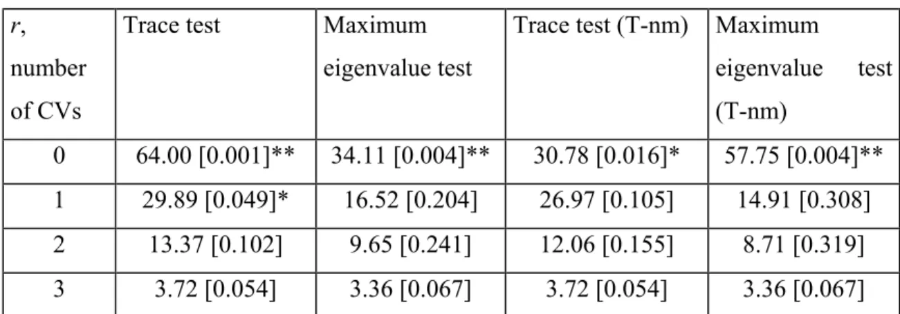
Table 4 summarizes results from four tests used to determine the number of cointegrating vectors (CV)22. In every case, the statistic presented and respective probability value correspond to the null hypothesis that the number of cointegration vectors, r, equals the figure in the first column. With the trace test, the number of cointegrating vectors exceeds r
21 See Doornik and Hendry (2000), vol. II.
under the alternative hypothesis. When applying the maximum eigenvalue test, the alternative is that the number of cointegrating vectors equals r+1. The tests denoted (T-nm) include a small sample correction suggested by Reimers (1992).
Table 4 Cointegration tests r,
number of CVs
Trace test Maximum eigenvalue test
Trace test (T-nm) Maximum
eigenvalue test (T-nm) 0 64.00 [0.001]** 34.11 [0.004]** 30.78 [0.016]* 57.75 [0.004]** 1 29.89 [0.049]* 16.52 [0.204] 26.97 [0.105] 14.91 [0.308] 2 13.37 [0.102] 9.65 [0.241] 12.06 [0.155] 8.71 [0.319] 3 3.72 [0.054] 3.36 [0.067] 3.72 [0.054] 3.36 [0.067]
Values within brackets are p-values. * Rejection at the 5 percent level. ** Rejection at the 1 percent level.
Even if one of the trace test results in Table 4 suggest that there could be two CVs, the other three tests clearly indicate that there is one, and one only, cointegrating vector. On the whole, results imply therefore that matrix Π in equation (15) has rank 1. Under this hypothesis, this matrix can be decomposed as:
', (16)
ab = Π
where a is a 4x1 vector of loadings and b is a 4x1 cointegrating vector. Estimation of the cointegration vector and ceteris paribus rates of return
Estimation of a cointegrated VAR by full information maximum likelihood imposing one cointegration relationship yielded results for the cointegrating vector parameters and their standard errors presented in Table 5, line 1.
Table 5
Estimated cointegrating vectors
Likelihood ratio test of restrictions Y H (γ) kg (β) kp (α) Estimated parameter -1.0 0.0563 0.148 0.557 Standard error 0.0 0.0643 0.373 0.198 1. No restrictions
Ceteris paribus r.o.r. 0.158 0.267 0.185 Estimated parameter -1.0 0.0660 0.294 0.350 Standard error 0.0 0.0 0.071 0.0 2. Imposed elasticity of kp and imposed semi-elasticity of H 2978 . 0 ) 2 ( 2 = χ (P-value: 0.8611)
Ceteris paribus r.o.r 0.154 0.568 0.090
The cointegrating vector was normalized imposing that the parameter associated with GDP equals -1. A production function interpretation of this vector associates the other parameters to elasticities (or to a semi-elasticity, in the case of H). Knowledge of these elasticities allows us to compute the ceteris paribus rates of return, also presented in the table23. Note that the estimated r.o.r. on private investment, of about 18.5 percent, is quite high. For instance, it is higher than recent estimates for the US economy24. The estimated public capital elasticity ensures a ceteris paribus r.o.r. for public investments, 26,7%, clearly above the private one. The estimated ceteris paribus rate of return on human capital formation results from all three parameters α, β and γ (see equation 11). It implies that this type of investment is fairly profitable – yielding a return of 15.8%, close to, albeit below, the private investment one. It is interesting to note that an even higher estimated elasticity for public capital is obtained if we jointly impose two restrictions on private and human capital production function parameters (Table 5, line 2). These restrictions are:
– a ceteris paribus r.o.r. on private capital equal to 9 percent (a figure closer to the estimates for the US economy), which, considering the private capital to output ratio in 2001, amounts to imposing α =0.35;
– a human capital semi-elasticity equal to 0.066. De la Fuente (2003) estimates the elasticity of output to average schooling years (call it ε ) to be comprised between 0.394 and 0.587, for a sample of EU countries. We arrived to the 0.066 value by
23 Rates of return on public capital were computed using 2001 values for Y/KG and δ (recall equation (4) and
taking the simple average between those two extremes and dividing it by the Portuguese level of average years of schooling in 2001 (since
H ε γ = ).
The joint hypothesis that γ and α is not rejected at a 86.11 percent level. The estimated elasticity of public capital is equal to 0.294, which gives a ceteris paribus public investment r.o.r. equal to 56.8 percent. These impressive values are still smaller than those estimated by Aschauer (1989a, 1989b) for the US economy and by Ligthart (2000) for Portugal. Even so, in further analysis we use the non-restricted cointegrated VAR (Table 5, line 1), which includes a lower estimate of the growth effects of public investment.
066 . 0
= =0.35
Impulse response functions and dynamic feedbacks rates of return
To estimate the dynamic feedbacks rates of return on public and human capital investment, one considers the IRFs generated by shocks to kg and H, respectively. Following standard practice in VAR analysis, economically interpretable (i.e., structural) shocks to those variables, orthogonal to each other and to other disturbances in the system, are recovered through appropriate identifying hypotheses.
It is assumed that public capital does not respond contemporaneously to any structural disturbances to the remaining variables in the VAR. Pereira (2000) made a similar assumption as regards public investment, on grounds of the lags involved in government decision-making – an argument shared by this paper. This is equivalent to an orthogonalisation of shocks using the well-known Cholesky decomposition, with kg ordered first.
As regards investment in human capital, the decision of whether to pursue further studies is viewed as potentially responsive to innovations in any of the remaining variables: for instance, shocks to output or to physical investment (private or public) may influence labor market conditions and thus the trade-offs between taking up a job or staying at school25. In turn, y, kp and kg are assumed to be only affected by innovations in H with a lag – a possible justification being that the economic benefits from a better-educated population are to be
24 Poterba (1997) finds that this rate is close to 8.5 percent and CBO (1998) mentions different studies where it
varies between 7 and 11 percent.
25 An output innovation may affect the overall unemployment rate, whereas shocks to investment may change
the relative supply of low-skilled versus high-skilled jobs (e.g. more jobs in construction associated to public investment in infrastructures).
reaped when students leave school and start working, rather than when they are still studying. In the context of the above Cholesky decomposition, this amounts to ordering H last. However, since the literature offers no guide for the identification of human capital innovations, a sensitivity analysis will be carried out by considering other possible orderings of variables.
Figure 6 to 9 depict the IRFs generated by a 0.01 shock to kg (i.e., a one percent increase in public capital per worker)26. The response of output is positive both in the short and in the long run: forty years into the future, when IRFs have essentially converged, output per worker is about 0.33 percent above the baseline (see figure 9). The original exogenous increase in public capital also induces further changes in other inputs. Apart from the response of public capital itself (see Figure 7), our results show that public capital innovations crowd in private investment (see Figure 8). The IRF of kp indicates that the private capital stock is approximately 0.32 percent above the baseline in the long run. On the other hand, public investment seems to crowd in human capital investment in the short run, but crowd it out in the long run – Figure 6 tells us that in the long run human capital is almost 0.003 years of schooling below the baseline.
The IRF of kg implies a time series of gross public investment deviations from baseline. This time series can be computed by converting the percentage deviations of public capital into absolute, constant euros terms (recall that kg is a log), and then using equation (13) with a depreciation rate of 4 per cent (as in section 4). After also converting the response of y into absolute terms, it becomes possible to compute the value of r that solves equation (5)27. This dynamic feedbacks r.o.r. on public investment equals 37.3 percent.
Comparing this result to the 15,9% r.o.r. computed by Pereira and Andraz (2002, 2004) for public investment in transportation infrastructures, it seems at first sight that our estimated return is almost 2.5 times bigger. However, though both figures take dynamic feedbacks into account, they are not comparable for a number of reasons: the VAR specifications are
26 In the context of a VAR in error-correction form – see equation (15) – the depicted responses are actually
accumulated IRFs. The same holds for the remaining IRFs of this section.
27 As the empirical analysis is set in discrete time, r is derived from the discrete-time counterpart of equation
(5), namely, . A similar discrete-time approximation will be used when computing the dynamic feedbacks r.o.r. on human capital.
∑ ∑ ∞ = ∞ = + ∆ = + ∆ 0 0 ) 1 /( ) 1 /( t t t b t t t bY r IG r
different; we consider all public investment, not just transportation infrastructures; most importantly, their r.o.r. is based on long-run impacts, while we consider the full path of dynamic responses (recall equation (5) and note 8). A better, albeit still imperfect, comparison can be made by looking at the “total marginal product” of public investment – the ratio between the long-run responses of the levels of output and public investment, both measured in constant euros. Pereira and Andraz (2002, 2004) report a value of 9.5, whereas we obtain 14.6 – still bigger, but by a much smaller margin.
Presenting a high r.o.r., it is hardly surprising to find that public investment pays for itself by generating additional fiscal revenues. For instance, assuming that in the Portuguese economy output is taxed at a rate of 35% (as in Pereira and Andraz, 2002), and government bonds pay interest at a rate of 6% (a figure close to the implicit rate on public debt in recent years), then public investment pays itself back in only 13 years, generating further revenues afterwards. Figures 10 to 13 present the impulse responses of H, kg, kp and y to a 0.01 shock in H (an increase of one hundredth of a year in the average years of schooling). One observes that, over time, there is a positive response of output (Figure 13), though of a very small magnitude – an increase of less than 0.03% in the long run. Figure 12 provides the clue to such a reduced impact: human capital investment is found to crowd out private physical investment, private capital per worker becoming almost 0.06% lower in the long run. The overall impact on output is therefore the net effect of the growth in H and in kg (which is crowded in to some extent – see Figure 11), and of the reduction in kp. One also remarks that there is some gradual weakening of the effort in human capital investment, more than 7 percent of the initial impulse being lost in the long run (see Figure 10).
To compute a dynamic feedbacks r.o.r. on human capital, one converts the gains in output per worker into constant euros (as in the case of public capital), generates a series for investment in human capital (simply the first difference of the IRF of H, since depreciation is ignored – see section 3), and translates it into euros per worker using equation (7). For the time span of the IRFs, the outcome is a modest r.o.r. of 2.7%.
As mentioned above, Cholesky decompositions with different orderings of variables were also considered. More specifically, kg was kept first throughout and shocks to H were simulated under all the possible orderings for the remaining variables (y, kp, H). The response of kp
(crowding out) was qualitatively similar to that reported above28 but generally stronger, leading to slight decreases in output (long run losses between 0.02 and 0.12 percent), and hence making it impossible to compute dynamic feedbacks r.o.r.
6. Conclusions
This paper has quantified the importance of both public capital and human capital for aggregate output in a unified, production function-based framework, rather than separately, as in previous studies. The Portuguese economy has been taken as a case study, due to the availability of annual time series for the several capital stocks involved. Resorting to the estimation of a cointegrated VAR model has made it possible to compute and compare two alternative concepts of rates of return, according to whether the dynamic feedbacks between the different production factors are considered or not.
Investment in public capital was found to yield a ceteris paribus return of 26,7%, well above the homologous figures for private capital (18,5%) and human capital (15,8%). Though seemingly uncommon, such a high figure simply stems from the estimated elasticity of output w.r.t. public capital – which, in turn, is actually lower than the corresponding estimates of other studies. Fears that public investment may crowd out private investment are not confirmed: instead, crowding in takes place, explaining the even higher return (37,3%) when dynamic feedbacks are accounted for. As for budgetary consequences, this study finds that public investment fully pays itself back in only thirteen years, while its positive influence on output and fiscal revenues is much more long-lasting.
A number of policy implications for the Portuguese economy ensues. First, the emphasis on infrastructural improvement laid since Portugal joined the European Union, and started to benefit from structural funds, seems well justified. Second, in the light of the political vulnerability of public investment in times of fiscal retrenchment, the empirical findings here reported lend support to fiscal frameworks that include a golden rule, and run against the counterargument that private capital is crowded out. Finally, and in a similar vein, fiscal consolidation efforts which fall disproportionately on public investment may severely hamper growth prospects, and are in all likelihood counterproductive even in narrow fiscal terms, due
to lost revenue. A caveat to be born in mind, however, is that in most of our sample period Portugal had a blatant infrastructural deficit, which is probably no longer the case, though insufficiencies persist. It cannot therefore be excluded, as Pereira and Andraz (2004) caution (p. 240), that in the future returns on public capital will become smaller.
Results for human capital were less clear-cut. Though the estimated ceteris paribus r.o.r. (15,8%) was fairly high, and close to private capital’s, shocks to years of schooling were found to induce a negative dynamic response of private investment, leading to a disappointing 2,7% return with dynamic feedbacks. Worse still, a sensitivity analysis revealed that the dynamic response of output could actually be negative. As in the case of public capital, some prudence is called for when interpreting these results. A first point to make is that one should not conclude that investment in human capital is almost “unproductive”, or even detrimental: the crowding out of private investment also means that the associated costs are not incurred29,
an aspect which the dynamic feedbacks r.o.r. fails to capture (recall the discussion in section 3)30. A second point, made by Barro (2001), among others, is that the quality of education may be at least as important as its quantity (i.e., the number of years at school). Attempting to capture the former, and not just the latter, seems an important avenue for future work.
It would also be interesting in future research to study other countries. As mentioned in the introduction, our motivations and methodology, unlike our data set, do not concern only Portugal.
29 And thus more resources are left available for other uses, such as consumption.
References
Aaron, H. (1990) Discussion. In Is There a Shortfall in Public Capital Investment? Proceedings of a Conference (A Munnell, Ed.). Boston: Federal Reserve Bank.
Aschauer, D. (1989a) Is public expenditure productive? Journal of Monetary Economics 23: 177- 200.
Aschauer, D. (1989b) Does public capital crowd out private capital? Journal of Monetary Economics 24: 171- 188.
Aschauer, D. (1990) Why is Infrastructure Important? In Is There a Shortfall in Public Capital Investment? Proceedings of a Conference (A Munnell, Ed.). Boston: Federal Reserve Bank.
Banco de Portugal (1997) Séries Longas para a Economia Portuguesa Pós II Guerra Mundial. Lisbon: Banco de Portugal.
Barro, R. (2001) Human Capital and Growth. American Economic Review 91(2): 12-17. Barro, R. and Lee, J. (2000) International Data on Educational Attainment: Updates and Implications. Working paper 7911, National Bureau of Economic Research, Cambridge, Massachusetts.
Batina, R. (1999) On the long run effect of public capital on aggregate output: Estimation and sensitivity analysis. Empirical Economics 24: 711-717.
Batina, R. (2001) The Effects of Public Capital on the Economy. Public Finance and Management 1(2): 113-134.
Blanchard, O. and F. Giavazzi (2004) Improving the SGP Through a Proper Accounting of Public Investment. CEPR Discussion Paper no. 4220, London.
Buti, M., S. Eijffinger and D. Franco (2003) Revisiting the Stability and Growth Pact: Grand Design or Internal Adjustment? CEPR Discussion Paper 3692, London.
Cohen, D. and M. Soto (2001) Growth and Human Capital: Good Data, Good Results. OECD Development Centre, Technical Papers no. 179. Organisation for Economic Cooperation and Development, Paris.
Congressional Budget Office (1998) The Economic Effects of Federal Spending on Infrastructure and Other Investments. CBO Paper, Congressional Budget Office, Washington. Crowder, W. and D. Himarios (1997) Balanced growth and public capital: an empirical analysis. Applied Economics 29: 1045-1053.
De la Fuente, A (2003) Human capital in a global and knowledge-based economy, Part II: assessment at the EU country level – final report. Brussels: European Commission, Directorate-General for Employment and Social Affairs.
De la Fuente, A. and A. Ciccone (2002) Human capital in a global and knowledge-based economy – final report. Brussels: European Commission, Directorate-General for Employment and Social Affairs.
De la Fuente, A. and R. Doménech (2000) Human Capital in Growth Regressions: How Much Difference Does Data Quality Make? Working paper nº 262, OECD Economics Department, Organisation for Economic Cooperation and Development, Paris.
Doornik, J. and D. Hendry (2000) Modelling Dynamic Systems Using PcGive. London: Timberlake Consultants.
Doornik, J. and D. Hendry (2001) GiveWin, An Interface to Empirical Modelling. London: Timberlake Consultants.
Evaraert, G. (2003) Balanced growth and public capital: an empirical analysis with I(2) trends in capital stock data. Economic Modelling 20: 741-763.
Flores de Frutos, R., M. Gracia-Díez and T. Pérez-Amaral (1998). Public capital stock and economic growth: an analysis of the Spanish economy. Applied Economics 30, 985-994. Gramlich, E. (1994). Infrastructure Investment: A Review Essay. Journal of Economic Literature 32: 1176-1196.
Hayashi, F. (2000). Econometrics. Princeton University Press, Princeton.
Johansen, S. (1988). Statistical analysis of cointegration vectors. Journal of Economic Dynamics and Control 12: 231-254.
Jones, C. (2002). Sources of U.S. Economic Growth in a World of Ideas. American Economic Review 92(1): 220-239.
Kamps, C. (2003). New Estimates of Government Net Capital Stocks for 22 OECD Countries 1960-2001. Working paper. Kiel Institute for World Economics, Kiel, Germany.
Krueger, A.B. and M. Lindahl (2001). Education and growth: why and for whom? Journal of Economic Literature 39: 1101-1136.
Lau, S. and P. Sin (1997). Public infrastructure and economic growth: time-series properties and evidence. Economic Record 73(221) June: 125-135.
Ligthart, J.E. (2000). Public Capital and Output Growth in Portugal: An Empirical Analysis. Working Paper 00/11, International Monetary Fund, Washington.
Lucas, R. E. (1988). “On the Mechanics of Economic Development”. Journal of Monetary Economics 22: 3-42.
Mankiw, N. G., D. Romer and D. N. Weil (1992). A Contribution to the Empirics of Economic Growth. Quarterly Journal of Economics 2(2): 407-437.
OECD (2003). Education at a Glance – OECD Indicators. Paris: Oganisation for Economic Co-Operation and Development.
Pereira, A. M. (2000). Is All Public Capital Created Equal? The Review of Economics and Statistics. 82(3): 513-518.
Pereira, A. M. and J. M. Andraz (2002). Public Investment in Transportation Infrastructures and Economic Performance in Portugal. In Portuguese Economic Development in the European Context: Determinants and Policies. Proceedings. Lisbon: Banco de Portugal.
Pereira, A. M. and J. M. Andraz (2004). O Impacto do Investimento Público na Economia Portuguesa. Lisbon: Fundação Luso-Americana para o Desenvolvimento.
Pereira, A. M. and O. Roca (2001). Public Capital and Private-Sector Performance in Spain: A Sectoral Analysis. Journal of Policy Modeling 23: 1-14.
Pereira, A. M. and O. Roca (2003). Spillover Effects of Public Capital Formation: Evidence from the Spanish Regions. Journal of Urban Economics 53: 238-256.
Pereira, J. (2003). A Medição do Capital Humano em Portugal. Master Thesis, Instituto Superior de Economia e Gestão, Lisbon.
Pina, A. and M. St. Aubyn (2002). Public Capital, Human Capital and Economic Growth: Portugal, 1977-2001. Working paper. Departamento de Prospectiva e Planeamento, Ministério das Finanças, Lisbon.
Poterba (1997). The Rate of Return to Corporate Capital and factor Shares: New Estimates Using Revised National Income Accounts and Capital Stock Data, Working paper 6263, National Bureau of Economic Research, Cambridge, Massachusetts.
Reimers, H.-E. (1992). Comparisons of tests for multivariate cointegration. Statistical Papers 33: 393-397.
Shwert, G.W. (1989). Tests for unit roots: A Monte Carlo investigation. Journal of Business and Economic Statistics 7: 147-159.
Sianesi, B. and J. Van Reenen (2002). The Returns to Education: A Review of the Empirical Macro-Economic Literature. Working paper nº 02/05, The Institute for Fiscal Studies, London.
Tatom, J. (1991). Public Capital and Private Sector Performance. Review of the Federal Reserve Bank of Louis 78(3): 3-15.
Teixeira, A. (1996). Capacidade de Inovação e Capital Humano. Master Thesis, Faculdade de Economia da Universidade do Porto.
Teixeira, A. and N. Fortuna (2003). Human Capital, Innovation Capability and Economic Growth, working paper no. 131, Faculdade de Economia da Universidade do Porto.
Appendix - Time series used in this paper
Year Employment GDP Human capital Public capital Private capital
1960 3743.599 18.194 2.237 8.086 34.842 1961 3726.690 19.142 2.284 8.494 36.699 1962 3716.545 20.406 2.337 8.850 39.052 1963 3705.273 21.605 2.401 9.283 41.213 1964 3695.127 23.175 2.471 9.745 42.807 1965 3683.855 24.928 2.552 10.185 44.683 1966 3661.310 25.889 2.641 10.593 47.056 1967 3638.765 27.980 2.732 11.034 50.178 1968 3616.220 30.547 2.827 11.394 53.191 1969 3593.675 31.576 2.928 11.793 56.345 1970 3789.816 33.973 3.051 12.286 59.981 1971 3778.544 36.209 3.121 12.706 63.780 1972 3754.872 39.122 3.210 13.148 68.714 1973 3723.309 43.513 3.312 13.614 75.070 1974 3694.000 44.000 3.436 14.129 81.928 1975 3724.000 42.100 3.539 14.522 89.219 1976 3789.000 44.998 3.653 15.003 93.686 1977 3784.000 47.482 3.775 15.616 97.181 1978 3772.000 48.819 3.936 16.272 102.028 1979 3854.000 51.572 4.091 17.093 106.021 1980 3940.000 53.939 4.261 18.107 110.807 1981 3918.000 54.812 4.450 19.349 114.422 1982 3928.000 55.982 4.539 21.010 118.812 1983 4128.000 55.885 4.678 22.273 123.450 1984 4075.000 54.835 4.789 23.273 127.634 1985 4057.000 56.374 4.911 24.064 130.263 1986 4059.700 58.708 5.046 24.748 132.601 1987 4148.200 62.455 5.177 25.480 135.197 1988 4252.400 67.132 5.309 26.376 139.665 1989 4346.700 71.456 5.457 27.553 145.422 1990 4438.500 74.279 5.610 28.716 151.172 1991 4562.700 77.523 5.765 29.891 157.449 1992 4468.400 78.368 5.911 31.167 163.814 1993 4389.000 76.767 6.116 32.809 170.547 1994 4381.600 77.507 6.321 34.570 174.772 1995 4358.400 80.827 6.519 36.100 178.749 1996 4388.400 83.690 6.704 37.713 182.804 1997 4477.300 87.007 6.868 39.713 186.901 1998 4597.599 90.992 7.028 41.915 192.794 1999 4683.735 94.450 7.169 43.879 200.609 2000 4784.265 97.933 7.313 46.138 208.738 2001 4848.412 99.540 7.433 48.033 217.197
Employment - Civilian domestic employment, 1000 persons. Source: AMECO, Annual macro-economic database of the European Commission's Directorate General for Economic and Financial Affairs (DG ECFIN), May 2004.
GDP – Gross domestic product at 1995 market prices, 109 euros. Source: AMECO, May 2004.
Human capital - Average years of schooling of the Portuguese population aged between 15 and 64. Source: Pereira (2003).
Private capital and public capital – Constructed by the authors. Values at 1995 prices, 109 euros. See main text
Figure 1
Figure 3
Figure 5
Figure 7
Figure 9
Figure 11