2D Cloud Template Matching - A comparison between Iterative Closest Point and
Perfect Match
H´eber Sobreira1
, Luis Rocha1
, Carlos Costa1
, Jose Lima1,3
, Paulo Costa1,2
, A. Paulo Moreira1,2 1
INESC-TEC, 2
Faculty of Engineering of University of Porto Rua Dr. Roberto Frias, 4200-465 Porto, Portugal
3
Polytechnic Institute of Braganc¸a
Campus Sta Apol´onia, 5301-857 Braganc¸a, Portugal
{heber.m.sobreira, luis.f.rocha, carlos.m.costa}@inesctec.pt, [email protected],{paco, amoreira}@fe.up.pt
Abstract—Self-localization of mobile robots in the
environ-ment is one of the most fundaenviron-mental problems in the robotics field. It is a complex and challenging problem due to the high requirements of autonomous mobile vehicles, particularly with regard to algorithms accuracy, robustness and computational efficiency. In this paper we present the comparison of two of the most used map-matching algorithm, which are the Iterative Closest Point and the Perfect Match. This category of algorithms are normally applied in localization based on natural landmarks. They were compared using an extensive collection of metrics, such as accuracy, computational effi-ciency, convergence speed, maximum admissible initialization error and robustness to outliers in the robots sensors data. The test results were performed in both simulated and real world environments.
Keywords-Autonomous Robots, Self-Localization,
Map-Matching, Iterative Closest Point, Perfect Match
I. INTRODUCTION
Industrial mobile robots (AGVs, Automatic Guided Ve-hicle), are nowadays vehicles that can self-localize and move autonomously without human intervention. Usually they are used to transport materials between work stations in warehouses and production lines.
AGVs are been used in industrial environments for more than 50 years and both the algorithms and hardware used has been evolving in order to increase the accuracy, robustness and flexibility while decreasing costs of the overall system. Regarding the localization systems, it is common to use sev-eral solutions such as line following and laser triangulation [2], [3]. Although, we are focusing in industrial autonomous robots (AGVs), the localization problem is transversal to all indoor autonomous robots application areas. Meanwhile, in the last decade localization based on natural marks has been increasing [4], [5]. These natural marks are composed by a set of distances and angles to the detected objects (such as doors, walls, furniture, ...) that can be acquired through an on-board laser range finder. This method has the main advantage of not requiring the installation of dedicated
reflectors in the environment, which in some factories might not be a viable option.
On the other hand, it is expected that even without special markers and straight corridors, the localization system re-mains robust. Besides these advantages, this approach needs to process a significant amount of sensor data efficiently in order to provide real-time localization. Therefore, the map-matching algorithms must be optimized in terms of accuracy, processing time, convergence speed and also sensor noise robustness.
The map-matching is a method of self-localization for mo-bile robots in which the local environment map (actual data acquired by the robot) is matched with and already stored map. With this in mind, this paper addresses the comparison of two of the most used algorithms in localization systems based on environment natural marks, which are the Perfect match (PM) [14] and the Iterative Closest Point (ICP) [17]. On the one hand the Perfect Match algorithm has increased its popularity within the robotics community mainly due to its successful application in the Middle Size League (MSL) robot soccer competitions in which it was able to provide robust localization for robots that require high frequency decision and locomotion control. On the other hand ICP is also one of the most used approaches to solve the map matching problem for 2D and 3D point-clouds. Moreover, its implementation is available in the Point Cloud Library (PCL), one of the most relevant open-source projects related to robotics.
The comparison and evaluation of both of these two algorithms will be performed considering different metrics, namely, the computational weight of each algorithm, the speed of convergence, the maximum admissible initializa-tion error (maximum error introduced in the initial pose estimation of the robot that the map-matching algorithms can tolerate), and finally the robustness of the algorithms in the presence of outliers on the robot sensors data.
For the execution of this comparison the ROS (Robot Operating System) framework was used. In this regard, the
work of Carlos et al. [1] was used to make the interface between ROS and PCL as it was designed to solve the robot localization problem and is completely parameterizable.
In terms of results, these were extracted both in a simulated environment (Stage Simulator) which virtually generated the sensory information of the robot (laser range finder data), as well as using a real robotic platform (Jarvis robot), which has a Sick NAV350 laser range finder on board used as ground-truth.
This paper is organized as follows: after the brief in-troduction given in this section, section 2 presents some related work. Then section 3 describes the algorithms (Per-fect Match and Iterative Closest Point) whereas section 4 addresses the comparison results based on an experimental setup. Finally, section 5 concludes the paper and presents some future work.
II. RELATEDWORK
For more than twenty years a wide scientific community has been dedicated to the localization problem of mobile robots. The extensive state of the art in this area has many proposed solutions based on different algorithms and different types of sensors. But, unfortunately, there are few commercial solutions and they are mostly used in very controlled environments.
In [6], Sabattini lists the weaknesses of existing logistics systems using AGVs and proposes several improvements. Among them is the robot localization using outlines. Based on this approach, in [7], [8] it is discussed its application based on the localization of three dimensional information extraction in an industrial environment. These articles are the result of the European project PAN ROBOTS. Also based on contours localization, Thrun in his book [9] describes an improved particle filter. This algorithm named AMCL (Augmented Monte Carlo Localization) has the character-istic of having a number of dynamic particles according to the pose uncertainty and furthermore it adds a global positioning strategy in order to perform the localization of the robot without no previous estimated location. However, the recovery of this global location only works well with a very high number of particles, which makes the algorithm computationally heavy. There are also other approaches to the problem of global localization, as can be seen in the work presented in [10], [11], [12], [13]. Martin Lauer et al. [14] presents a matching algorithm from a set of points and an occupancy grid. This has been adopted by many of the teams participating in the robot soccer leagues, given the computational light algorithm which allow the use of high frequency control loop in robots. Furthermore, in [14] it is also made a comparison between this algorithm and one based on particle filter, where Perfect Match proved its com-putational efficiency. Using this same algorithm, M. Pinto et al. [4] presented a localization system for an indoor service robot (surveillance) which performs localization based on
the roof contours. In this reference a comparison to the ICP algorithm is also given, but not with as much detail as we will present in the present article.
There were other works presented over the years for solving the map-matching problem. One of the most used category of these algorithms is the Iterative Closest Point (ICP) [15]. This algorithm iteratively searches for the rigid transformation that best aligns two sets of points. Lu and Milios presents in [16] an application of ICP with the data obtained from a laser range finder. Along the same topic there is the Iterative Closest Line (ICL) algorithm [17], where the matching is done between a set of points and a set of lines. The major disadvantage of all these algorithms is the high computational effort of correspondence search between the two sets of points, because this demand has to be done at each iteration. The Polar Scan Matching (PSM) [18] avoids this demand matching taking advantage of the polar nature of a laser scanner measures. Finally, we also refer the Vasco algorithm available on the open-source CARMEN library that consists of a set of successive approximations, until the test step is below a certain value. Until now, the presented matching algorithms are based on a search for a local minimum assuming that the solution cor-responds to the global minimum. However, such approaches can have problems if the initializing error is high. Therefore, on the opposite way to what was presented until now, Olson et al. [19] shows an exhaustive search made throughout all space solutions. The authors believe that using a set of optimizations it is possible to use this algorithm for real-time applications, supporting it with a set of comparative results (based on execution times) with other algorithms.
III. ALGORITHMS DEFINITION
In this section the main concepts of the algorithms used in the comparison will be presented. First we will start with the Perfect Match.
y direction. The first gives the direction of the variation of the distance map with the variation of thex position. The second shows the direction variation of the distance map with the y position variation. These three maps (gradient and x/y matrices) can be pre-computed in order to speed up the computation of the Perfect Match algorithm.
Considering now a list of points of a Laser Range Finder scan defined asP List. The pointiof this list in the world referential frame is P List(i) = (xi, yi). The cost value is given 1 wheredi andEi represents the distance matrix and cost function values of the pointi.
E=
P List.Count
i=1
Ei, Ei= 1−
L2 c
L2 c+d
2 i
(1)
The parameterLcis used to discard points with large error
Ei, increasing the robustness of the algorithm to outliers. To minimize the error function, the Perfect Match algorithm uses the RPROP optimizer. The output of this algorithm will be the state of the robot, x,y and θ (robot pose) that minimizes the map-matching error. For a detailed description of the algorithm please refer to [14].
2) Iterative Closest Point: The iterative closest point algorithm, is a commonly used matching/registration al-gorithm, which tries to minimized the Euclidean distance between the input data and a reference model (in the self-localization problem it corresponds to the laser range finder data and the map of the environment).
From a mathematical point of view, consider two sets of 2D points, source A (with n points) and target B (with
m points)⊆ R2
. The objective is to find a transformation function u : A → B that minimizes the mean squared distances (MSD) betweenAand B (see (2)).
M SD(A, B, u) = 1
n
a∈A
a−u(a)2
(2)
Incorporating the rotation (R) and translation (t) matrices into the matching function and assumingu(ai) =bi where
ai∈Aandbi∈B, the minimization problem can be written using 3.
min
u:A→B
1
n
n
i=1
Rai−t−bi 2
(3)
With this mathematical formulation, the ICP tries in each iteration to minimize the M SD(A, B, u), by alternating between a matching and a transformation stage.
Matching stage: In this first stage, the objective is to minimize theM SD(A, B, u) by finding the best direct correspondence between a point ai ∈A and bi ∈ B. This step is in its most basic form executed by selecting the point
bi ∈ B with the minimum Euclidean distance to the point
ai∈A(Voronoi diagram). Note that in the first iteration,t andRare normally set to[0,0]T and to the identity matrix respectively.
Transformation stage: During the transformation stage, the objective is to compute the optimal R and t that minimizes (3), using the correspondence matrix computed in the previous step. ICP uses a simple least square solver to find the optimal linear transformation matrix (R|t) that minimizes (3) [20]. For this purpose, the algorithm starts by computing the two centroids and subtracting it to the two point sets (shown in 4 and 5).
a′ i=ai−
1
n
n
i=0
ai (4)
b′ i=bi−
1
m
m
i=0
bi (5)
This step helps simplifying the minimization problem [20]. Then, the cross-variance matrix is computed using 6 withA′andB′being the set of pointsa′
iandb ′
irespectively.
H=A′B′T (6)
Now, the rotation angleθcan be computed from equation 7.
θ=atan2((H(0,1)−H(1,0)),(H(0,0) +H(1,1)) (7)
It can be shown that the optimal solution for R and t
that minimizes the objective function is given by 8 and III-2 where¯aand¯bare the points centroid computed in equation 4 and 5. In the end of this Matching stage, the algorithm goes back to the transformation stage, and both are performed until a stopping criteria is verified (e.g. number of iterations, Euclidean error improvement between iterations, etc).
R=
cos(θ) −sin(θ)
sin(θ) cos(θ)
(8)
t= ¯b−Ra¯ (9)
The ICP 2D implementation used in this paper was the one available in the Point Cloud Library (PCL).
IV. EXPERIMENTALRESULTS
1) Framework description and evaluation tests: The ROS framework was used to perform the comparison of the Per-fect Match and ICP algorithms. Considering the simulation case, the STAGE simulator was selected since it allows to model a virtual world where it can be introduced robots, sensors and objects. This simulator has available a version that is already integrated with ROS. Besides the simulation, it is also presented results with a real robot platform (Jarvis). This robot is equipped with a commercial navigation laser (SICK NAV350) seen in Figure 1.
Figure 1. Jarvis Robot
2) Set-up of the experiment: The initial parametrization of the algorithms for all the experiments was made as follows:
• Both algorithms process the same amount of data • Both algorithms use the same reference map • Both algorithms use the same stopping metrics • Both algorithms do not have access to data from
odometry. Therefore the pose error is caused by the robots movement, traveling at 0.5 m/s
• The version of the ICP available in PCL used
in the tests is ”iterative closest point 2d”
available in [1], without RANSAC
(”max number of ransac iterations : 0”), and to ensure that all data are processed, the maximum distance search value is set to a high value (”max correspondence distance: 9999.0” )
• The computer used had a Intel Core i7-2677M Dual
Core processor
3) Results on Computational Weight: In these first tests the main objective is to evaluate the computational weight of the algorithms. We intend to analyze the computational weight of an iteration of the ICP, i.e, the performance of point correspondence (based on Kd-tree for the PCL imple-mentation), and the optimization based on least squares; and
for the Perfect Match, i.e. , gradient computation based on look-up tables and the optimization based on RPROP.
In order to not penalize neither the results of each algo-rithm we fixed the number of iterations (50), also we do not use filters and other algorithms that may influence the evaluation of the computational weight.
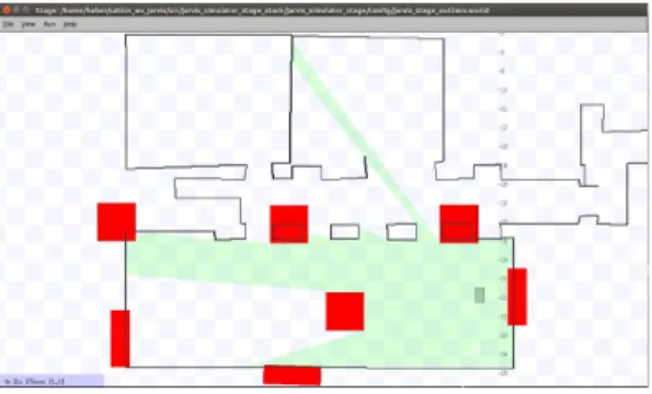
Furthermore, tests were made to analyze the influence in the computational weight of the number of the LIDAR points, the reference map size and the presence of noise in the sensors data (please refer to Figure 2). Only simulation results are presented for these initial tests.
Figure 2. Stage Simulator with outliers presented in red color
Table I
COMPUTATIONAL TIME(IN MS)TAKEN BY EACH ALGORITHM TO PERFORM50ITERATIONS
results
Points 1440 Points 288
No Outliers Outliers No Outliers No Outliers No Outliers Outliers
Mean Time 61 63 274 131 355 478
Max Time 183 189 338 222 545 799
Min Time 54 55 252 119 332 398
Mean Time 1 1 3 1 5 4
Max Time 2 2 11 3 16 10
Min Time < 1 < 1 2 < 1 < 1 2 PM
Map Resolution 5cm Map Resolution 1cm Points 288 Points 1440
ICP
0 5 10 15 20 25
0 20 40 60 80 100 120
Number of
it
er
a
tions
Time (s) PM ICP
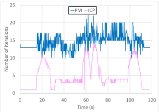
Figure 3. Number of iterations performed by ICP and PM
As future work about this topic we intend to analyze the distribution of time used by ICP in the search for corre-spondences and during the optimization. In an preliminary analysis we observed that in the case of the experiment in which ICP had worse results (map with higher resolution and sensor data with more measurements and with outliers) 75 percent of the time is spent searching for correspondences in the map kd-tree.
4) Results on Convergence Speed: At this point we have concluded that each ICP iteration (considering the PCL im-plementation), can be up to 113 times slower than a Perfect Match iteration. But this raises the question of convergence speed. The ICP may have a higher computational cost for each iteration, but it requires less iterations to converge on a good solution.
In order to analyze the convergence speed, it was added another stopping criteria in the two map-matching algo-rithms. This criteria evaluates the position and orientation corrections made by the algorithms between two iterations. If they are below a certain value the optimization process stops. The parameters values used in this stopping criteria were 0.01m in translation and 0.8 degrees in rotation for both algorithms. The selected test scenario was the one with less density in robot sensor data, and with the map with the lowest resolution and without outliers.
In Figures 3 and 4 are presented the results for the experiment described earlier.
Figure 3 presents the number of ICP (red) and PM (blue) iterations over time while the robot performs the path shown in Figure 5 while Figure 4 represents the ICP (in red) and PM (blue) convergence time while the robot performs the path shown in 5.
As can be seen in figure 3 the ICP algorithm needs less iterations than the PM to perform map-matching, but this is not enough to be lighter than Perfect Match.
In figure 4 it is also possible to identify three situations. A zone where the ICP performs only one iteration that corresponds to the situation that the robot is stopped. A zone where ICP performs about four iterations that corresponds to the situation where the robot is moving in a straight line.
0 10 20 30 40 50 60 70 80 90
0 20 40 60 80 100 120
Con
v
er
g
ence time
(ms)
Time (s) PM ICP
Figure 4. Execution times of ICP and PM
Figure 5. Interval for the rotation initial error that the algorithms support and still converge to a good solution. In purple results for the ICP and in blue color results for the PM
And another area where the number of iterations rises, even exceeding the PM number of iterations, corresponding to the situation when the robot is rotating. The above findings do not change if we repeat the experience for the scenario where there are outliers.
5) Maximum initialization error: In the presented tests the Perfect Match has show to be computationally lighter than ICP. In this section we will show test results for both algorithms considering the initial localization error of the robot, in order to evaluate which algorithm is more robust to local minima. In these experiences were used the same parameters of section IV-3, i.e, a fixed number of iterations was set and the maximum corresponding distance of ICP was set to a high value. In order to see the orientation error tolerance of the analyzed algorithms we have stopped the robot in some points of the robot trajectory and then both algorithms were reinitialized with an initial pose with a gradually greater orientation error (1 degree of resolution) until the matching algorithm diverges.
In Figure 5 it is presented the set of poses where these tests were performed (black arrows). Each of these poses have another two pairs of arrows (purple and blue). These correspond, respectively, to the ICP and PM orientation error limits in which they still converge to a correct solution.
0 0,05 0,1 0,15 0,2 0,25
0 20 40 60 80 100
P
osition err
or
(m)
Time (s)
PM ICP
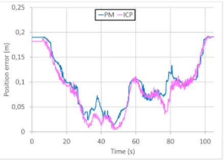
Figure 6. Position error along the trajectory with outliers in simulation
-1 -0,8 -0,6 -0,4 -0,2 0 0,2 0,4 0,6 0,8
0 20 40 60 80 100
Orien
ta
tion err
or
(degr
ees)
Time (s)
PM ICP
Figure 7. Orientation error along the trajectory with outliers in simulation
perform the experience setting the stopping criteria used in section IV-4 and limiting the correspondence distance of ICP but did not obtain better results.
6) Evaluation of the algorithms robustness to outliers: At this point we noted PM advantages in the computational weight. However, it is raised the question of accuracy and robustness to outliers. There exists a large number of studies that address this issue. In particular the use of the RANSAC for identifying the presence of outliers in the sensor data. But many of these methods are transversal to all matching algorithms and so it can be also used in the PM algorithm. We are only interested for now in analyzing the core algorithms, and we want to examine whether the PM computational efficiency is achieved by sacrificing accuracy / robustness to the result of matching.
The PM has built in its optimization function a kind of outlier filter, tuned by theLcparameter. In these experiments we used Lc = 1 meter. And to try to make this a more fair comparison we changed the ICP parameter of the maximum correspondence distance to 1 meter.
As it is possible to see in Figures 6 and 7, ICP has a mean position error of 0.097 m whereas the PM algorithm has a mean error of 0.106 m. We could not conclude with certainty that ICP is more robust because the ”filter” of maximum correspondence distance can also be used in the PM algorithm. However, we can conclude that the PM is computationally lighter with similar results in terms of accuracy and robustness. Leaving time for the application of more advanced filters in order to increase the efficiency of a localization algorithm that uses the PM.
-0,005 0 0,005 0,01 0,015 0,02 0,025 0,03 0,035
0 50 100 150 200
P
osition err
or
(m)
Time (s)
PM ICP
Figure 8. Positional error along the trajectory - Jarvis robot
-0,5 -0,4 -0,3 -0,2 -0,1 0 0,1 0,2 0,3 0,4 0,5
0 50 100 150 200
Orien
ta
tion err
or
(°)
Time (s)
PM ICP
Figure 9. Orientation error along the trajectory - Jarvis robot
At this point all the experiments were carried out in sim-ulation. But often simulators do not model important details that can make a significant difference in the performance of an algorithm. As such, we repeated the above experiments with a real robot equipped with a laser range finder with a reflective triangulation system installed on walls to serve as ground-truth.
All findings from previous experiments presented in sim-ulation are confirmed with the real robot. Figures 8 and 9, present the precision and results for the ICP and the PM in a real environment with the natural presence of outliers (in the same map of Figure 5).
V. CONCLUSIONS AND FUTURE WORK
This paper presented a comparison between two well known map-matching algorithms, the Perfect Match and the Iterative Closest Point. The Perfect Match shown to be much lighter than ICP in terms of computational cost, mainly due to its search data structures (look up tables) being more time efficient than the Kd-trees used in the PCL implementation of ICP. In the future we intend to integrate the look up tables search approach into ICP in order to compare the ICP optimization based on SVD with the RPROP used in the PM algorithm.
11.4 degrees in the robots pose, ICP needs 46 iterations to converge while PM only needed 29 iterations.
The analyses of the maximum initialization error was the most interesting result from the set of tests performed. The PM presented a much higher tolerance to orientation errors than ICP. As future work we intend to refine this result in order to also include position error. However, some preliminary tests were made which showed a similar response of the two algorithms in terms of translation error. In terms of accuracy, the two algorithms showed similar results, However the ICP and the PM implementation of how to handle outliers were not exactly the same. The PM has contemplated in its cost function the possible presence of outliers, while ICP handles outliers by trimming points that are farther than a given distance.
We know there are several solutions in the state of art. This study served to validate the relevance of PM and we intend this to be the basis for future developments. We also intend to extend this analysis to a larger number of algorithms and testing conditions and environments.
ACKNOWLEDGMENT
Project ”NORTE-01-0145-FEDER-000020” is financed by the North Portugal Regional Operational Programme (NORTE 2020), under the PORTUGAL 2020 Partnership Agreement, and through the European Regional Develop-ment Fund (ERDF).
REFERENCES
[1] Carlos M. Costa, H´eber M. Sobreira, Armando J. Sousa, Germano M. Veiga, Robust 3/6 DoF self-localization system with selective map update for mobile robot platforms, Robotics and Autonomous Systems, Volume 76, February 2016, Pages 113-140, ISSN 0921-8890,
[2] Schulze and A. Wullner, The Approach of Automated Guided Vehicle Systems, in 2006 IEEE International Conference on Service Operations and Logistics, and Informatics, 2006, pp. 522527.
[3] L. Schulze, S. Behling, and S. Buhrs, Automated Guided Ve-hicle Systems: a driver for increased business performance, in Proceedings of the International MultiConference of Engineers and Computer Scientists, 2008, pp. 1921.
[4] M. Pinto, H. Sobreira, A. Paulo Moreira, H. Mendonc¸a, and A. Matos, Self-localisation of indoor mobile robots using multi-hypotheses and a matching algorithm, Mechatronics, vol. 23, no. 6, pp. 727737, Sep. 2013.
[5] N. Tomatis, BlueBotics: Navigation for the Clever Robot [Entrepreneur], IEEE Robot. Autom. Mag., vol. 18, no. 2, pp. 1416, Jun. 2011.
[6] L. Sabattini, V. Digani, C. Secchi, G. Cotena, D. Ronzoni, M. Foppoli, F. Oleari, C. Reinke, and P. Beinschob, Technological roadmap to boost the introduction of AGVs in industrial applications, in Proceedings - 2013 IEEE 9th International Conference on Intelligent Computer Communication and Pro-cessing, ICCP 2013, 2013, pp. 223227.
[7] C. Reinke and P. Beinschob, Strategies for contour-based self-localization in large-scale modern warehouses, IEEE 9th Int. Conf. Intell. Comput. Commun. Process. ICCP 2013, pp. 223227, 2013.
[8] P. Beinschob and C. Reinke, Strategies for 3D data acquisition and mapping in large-scale modern warehouses, in Proceed-ings - 2013 IEEE 9th International Conference on Intelligent Computer Communication and Processing, ICCP 2013, 2013, pp. 229234.
[9] S. Thrun, W. Burgard, and D. Fox, Probabilistic robotics. Cambridge, MA: MIT Press, 2005.
[10] L. Zhang, R. Zapata, and P. Lpinay, Self-adaptive Monte Carlo localization for mobile robots using range finders, Robot-ica, vol. 30, no. 02, pp. 229244, Jun. 2011.
[11] A. R. Vahdat, Mobile robot global localization using differen-tial evolution and particle swarm optimization, in 2007 IEEE Congress on Evolutionary Computation, 2007, pp. 15271534.
[12] S. Thrun, M. Beetz, M. Bennewitz, W. Burgard, A. B. Cremers, F. Dellaert, D. Fox, D. Hhnel, C. Rosenberg, N. Roy, J. Schulte, and D. Schulz, Probabilistic algorithms and the interactive museum tour-guide robot Minerva, Int. J. Rob. Res., vol. 19, no. 11, pp. 972999, 2000.
[13] Z. Liu, Z. Shi, M. Zhao, and W. Xu, Mobile robots global localization using adaptive dynamic clustered particle filters, in 2007 IEEE/RSJ International Conference on Intelligent Robots and Systems, 2007, pp. 10591064.
[14] M. Lauer, S. Lange, and M. Riedmiller, Calculating the perfect match: an efficient and accurate approach for robot self-localization, Rob. 2005 Robot soccer world cup, no. c, pp. 142153, 2006.
[15] P. J. Besl and H. D. McKay, A method for registration of 3-D shapes, IEEE Trans. Pattern Anal. Mach. Intell., vol. 14, no. 2, pp. 239256, 1992.
[16] F. Lu and E. Milios, Robot Pose Estimation in Unknown Environments by Matching 2D Range Scans, J. Intell. Robot. Syst. Theory Appl., vol. 18, no. 3, pp. 249275, 1997.
[17] A. Censi, An ICP variant using a point-to-line metric, in 2008 IEEE International Conference on Robotics and Automation, 2008, pp. 1925.
[18] A. Diosi and L. Kleeman, Fast Laser Scan Matching using Polar Coordinates, Int. J. Rob. Res., vol. 26, no. 10, pp. 11251153, Oct. 2007.
[19] E. B. Olson, Real-time correlative scan matching, in IEEE International Conference on Robotics and Automation, 2009, pp. 43874393.