REM WORKING PAPER SERIES
Assessing the Sustainability of External Imbalances in the
European Union
António Afonso, Florence Huart,
João Tovar Jalles, Piotr Stanek
REM Working Paper 001-2017
September 2017
REM – Research in Economics and Mathematics
Rua Miguel Lúpi 20, 1249-078 Lisboa,
Portugal
ISSN 2184-108X
Any opinions expressed are those of the authors and not those of REM. Short, up to two paragraphs can be cited provided that full credit is given to the authors.
Assessing the Sustainability of External
Imbalances in the European Union
*António Afonso,
$.Florence Huart,
+João Tovar Jalles,
#Piotr Stanek
±2017
Abstract
We assess the sustainability of the current account (CA) balance, net international investment position (NIIP) and net external debt (NED) in a sample of EU countries using two complementary approaches. First, we employ both time-series and panel-data stationarity tests of current account balance-to-GDP ratios as well as cointegration tests of exports and imports of goods and services. Second, we assess the level of trade balance that stabilizes the NIIP and the NED. We find that there is sustainability of the CA balance mainly in a few surplus countries whereas there is more concern about the sustainability of the NIIP or NED in countries with a credit position than in countries with a debit position. Both approaches are consistent with each other given the relationship between flows and stocks, the existence of important structural breaks, and valuation effects via the exchange rate.
Keywords: current account, exports, imports, net foreign assets, unit roots, structural breaks, cointegration, error-correction, cross-sectional dependence European Union.
JEL Codes: C22, C23, F32, F34, F36, F41.
* We thank Pierre Aldama, Mario Alloza, Georgios Chortareas, Jérôme Creel, Etienne Farvaque, Bernd Hayo, Céline Tcheng, Pauline Wibaux, and participants at the Workshop “External imbalances: causes, consequences and rebalancing”, 2016 (Lille), at the INFER 19th Annual Conference, 2017 (Bordeaux), at the 6th UECE Conference on Economic and Financial Adjustments, 2017 (Lisbon), and at the 33rd International Symposium on Money, Banking and Finance, annual meeting of the European Research Group (GdRE) on Money Banking and Finance, 2017 (Nanterre), and at the Money, Macro and Finance Research Group Annual Conference, 2017 (London), for very useful comments. The usual disclaimer applies and all remaining errors are the authors’ sole responsibility. The opinions expressed herein are those of the authors and not of their employers.
$ ISEG – School of Economics and Management, Universidade de Lisboa; REM – Research in Economics and Mathematics, UECE. UECE – Research Unit on Complexity and Economics is supported by Fundação para a Ciência e a Tecnologia. email: [email protected].
+ LEM – CNRS (UMR 9221), University of Lille 1, Faculté des Sciences Economiques et Sociales, Villeneuve d’Ascq. 59655 Cedex France. E-mail: [email protected].
# Centre for Globalization and Governance, Nova School of Business and Economics, Campus Campolide, Lisbon, 1099-032 Portugal. UECE – Research Unit on Complexity and Economics. email: [email protected] ± Cracow University of Economics, email: [email protected].
1. Introduction
Following the Global Financial Crisis (GFC), the Euro Area (EA) crisis highlighted the need to improve macroeconomic surveillance in the European Union (EU) not only with regard to the nature of macroeconomic imbalances but also with regard to the institutional framework. Besides concerns about public deficits and public indebtedness, there has indeed been increasing attention to other sources of disequilibria such as external imbalances (current account balances and indebtedness of the nation).
In addition, the European Commission’s (EC) Macroeconomic Imbalance Procedure (MIP), established in 2011, is based on an alert mechanism, and uses a scoreboard of headlines indicators with indicative thresholds that intend to cover potential sources of macroeconomic imbalances. One of such indicators is the current account imbalance, which is assessed via a 3-year backward moving average of the current account balance (in percent of GDP), with thresholds of +6 percent and -4 percent1, and also a net international investment position (NIIP) (in percent of GDP), with a threshold of -35 percent.23 As far as the current account deficit is concerned, thresholds were derived from a statistical distribution analysis of the size of the current account deficit at a time of large current account reversal. As for the NIIP, a statistical distribution analysis was also carried out, but European Commission (2012a) does not give any details nor explanations.4 Hence, it becomes paramount notably for EU countries, to understand how far an economy might be from a sustainable external position. In fact, by ensuring the
1 According to Eurostat data, in the first quarter of 2016 eleven EU countries where breaching those thresholds. 2 The net external debt (NED) is an auxiliary indicator of the scoreboard with no threshold that is used for complementing the economic interpretation of the NIIP. Recall that the difference between NIIP and NED is that in the latter the position of direct investment (non-debt components) and financial derivatives are not counted. In economic terms, the NED gives information on potential risks insofar as debt liabilities have to be repaid at a certain point in time.
3 European Commission (2012a), dedicated to the set-up of the scoreboard, gives some information about the choice of the thresholds. It is worth knowing where do the values of these thresholds come from, because whenever an EU member country is out of line, the EC has to make some recommendations based on a macroeconomic analysis carried out in a country report, and the member country concerned has to implement economic policy measures in order to address these recommendations.
sustainability of the current account balance, countries are also contributing to meet the headline thresholds implicit in the EC’s Macroeconomic Imbalance Procedure.5
Against that backdrop, this paper assesses the sustainability of external imbalances in a sample of EU countries. We consider the sustainability of both external deficits and external surpluses, because the MIP aims at avoiding growing external surpluses as well.6 Implicitly, the idea is that the burden of adjustment for deficit countries would not be so high if current account surpluses in surplus countries were not that large. Indeed, the persistence of large current account surpluses in some EA countries (notably Germany, Netherlands, and Luxembourg) may go along with weak domestic absorption and low inflation. This can lead to an appreciation of the euro and make external rebalancing harder for deficit countries.7 Furthermore, even if the export structure of EA periphery economies might not be suitable to respond to higher domestic consumption or investment in Germany, those countries could nevertheless export more to Germany’s main trading partners if the latter could benefit from higher demand from Germany.
Our analysis is two-fold. First, we use the intertemporal current account constraint as a theoretical framework underlying the different tests of stationarity of current account-to-GDP ratios (also allowing for structural breaks). In that context we also test for cointegration between exports and imports of goods and services (ratios to GDP), along the lines of the works by Trehan and Walsh (1991) and Afonso (2005). For this approach, we rely on quarterly data for 22 EU countries over the period 1970:Q1-2015:Q4. To our knowledge, such tests have not been carried out for a large sample of EU countries and let alone over a period covering the EA crisis. The literature dealing with external debt sustainability has mainly focused on a subset of OECD
5 For the EA, Bénassy-Quéré (2016) discusses the current objectives in relation to the improvement of the fiscal stance. Afonso et al. (2013) address the relevance of the links between fiscal and current account imbalances. 6 The European Commission has not set any threshold for NIIP in credit position. Nevertheless, we look at the sustainability of NIIP and NED in countries with credit positions as well as in countries with debit positions, because persistent CA surpluses go along with persistent positive (negative) NIIP (NED).
countries, the United States alone, or emerging economies in America and Asia (see section 2 for details). Moreover, we propose an extensive set of (panel data) tests that take into account multiple (endogenously determined) structural breaks using recent techniques that also address cross-sectional dependence, which to our knowledge has never been applied in this area.
Second, we use the dynamic external debt constraint to assess the trade balance-to-GDP ratio that stabilizes the net foreign assets-to-GDP ratio (predicted or stabilizing trade balance). This section of the paper draws from the analysis of the “operational solvency condition” by Milesi-Ferretti and Razin (1996). An original feature of our approach is to consider not only that foreign assets are not necessarily denominated in foreign currency but also that foreign liabilities are not necessarily denominated in domestic currency as it is commonly done in the literature (based on the case of the United States). We thus introduce two new parameters, which cover the share of foreign assets denominated in foreign currency in total foreign assets, and the share of foreign liabilities denominated in foreign currency in total foreign liabilities. With such parameters, we can highlight the role of valuation effects through the exchange rate in the dynamics of net foreign assets (NIIP or NED), and particularly in the size of the predicted trade-balance.8 Due to data availability constraints, in this exercise, we are bound to use annual data over the period 1995-2015 (23 EU countries).
The remainder of the paper is organized as follows. Section 2 reviews the literature. Section 3 outlines the analytical framework. Section 4 explains the empirical analysis and discusses the main results. The last section concludes.
2. Literature
We can identify three main strands of literature that deal with the analysis of sustainability of external imbalances: 1) time-series and panel data behavior of trade balance,
8 Our paper does not explain the “original sin” (the inability of a country to borrow in its own currency), but focuses on the macroeconomic effects of “currency mismatch” (the differences in the currencies in which foreign assets and liabilities are denominated). For further details, see Eichengreen et al. (2003).
current account or external debt; 2) macroeconomic determinants of the dynamic external debt constraint; and 3) growth effects of external debt. Our work falls under the first two branches. There are numerous empirical studies relying on time series analysis to address the topic under scrutiny. The main idea is that if the current account is stationary, then the intertemporal budget constraint of the country holds (see Section 3.1). In the supplementary material, we provide a review of recent contributions to the literature dealing with OECD countries.9 There are two main empirical strategies commonly used: unit root tests and cointegration tests (Raybaudi et al., 2004; Holmes, 2006; Chen, 2011; Camarero et al., 2013), and error-correction models (Durdu et al., 2013; Bajo-Rubio et al., 2014).
Some researchers use nonlinear approaches, such as structural breaks, regime shifts or threshold values. In Chen (2014), various linear and nonlinear tests in CA/GDP series pointed to sustainability in a sample of ten OECD countries. Camarero et al. (2015) tested for the presence of structural breaks in the net foreign assets (NFA) series in 11 EA countries. The null of stationarity was not rejected for the panel for five countries only over the period 1972-2011.
Error-correction models are also used following the approach of fiscal reaction functions advocated by Bohn (2007) in the study of public debt sustainability. Specifically, a sufficient condition for the intertemporal constraint to hold is that there is a negative relationship between net exports and NFA. However, these reaction functions are estimated while taking for granted that net exports could be treated as a variable under the control of countries’ authorities (just like the primary balance in the literature on government debt sustainability).
The literature on time series analysis points to sustainable external imbalances as long as OECD countries or advanced countries are taken as a group. Such results tend to hold for a period preceding the GFC and Euro Area crisis. Yet the NFA position of some countries has
9 We do not review empirical studies covering the United States only (for that see Edwards, 2005) nor periods before the 2000s (for that see the review by Bajo-Rubio et al., 2014). A summary of recent papers is also provided in Chen (2011).
deteriorated markedly since the onset of the crisis. Moreover, at the individual country level, empirical findings are not conclusive (see details in Table A1). We aim at investigating the issue of external debt sustainability by taking into account the impact of the crisis not only at a group level but also at a country level. We also widen our sample to most of the EU countries.
Regarding the determinants of the dynamic external debt constraint, for instance Milesi-Ferretti and Razin (1996) argued that the intertemporal external debt constraint was not sufficient to assess the external debt/current account deficits sustainability. They put forward the factors influencing the willingness to pay the debt by the indebted country and the willingness to lend by foreign investors. They also used a dynamic debt constraint based on the balance-of-payment identity between the current account balance and the evolution of the stock of net foreign assets. The dynamic external debt constraint can be used to assess the trade balance, which is consistent with a stable external debt-to-GDP ratio, and to analyse the role of macroeconomic variables in the dynamics of debt. Using the equation of the predicted trade balance (stabilizing trade balance), one can compare the actual trade balance with the predicted one (current account gap), and assess the extent of the required macroeconomic adjustments.
Some studies have focused on the current account gap. Corsetti et al. (1999) used this approach in the context of the Asian crisis. Chortareas et al. (2004) applied it to Latin American countries. The European Commission (2012b) used it for eight EA countries with large negative NIIPs. However, in these studies, computations are made without taking into consideration valuation effects of exchange rate changes on the NIIP. We aim to address this problem (see Section 3.2).
Other studies in this literature have focused on the required macroeconomic adjustments. Many works have been done since the early 2000s to assess what would be the required depreciation of the dollar to stabilize the NIIP of the United States (see a review in Edwards, 2005). In particular, the exchange rate adjustment of the U.S. dollar could cause a
large negative wealth effect on European countries depending on their NFA position and the weight of the dollar in their foreign assets and liabilities (Obstfeld and Rogoff, 2005; Lane and Milesi-Ferretti, 2007).
3. Analytical Framework
3.1. Present Value Borrowing Constraint
In order to assess the sustainability of external imbalances we use the so-called present value borrowing constraint, along the lines set up notably by Trehan and Walsh (1991) and Hakkio and Rush (1991) for the assessment of the sustainability of both external and fiscal imbalances. The budget constraint in period t is given by the following equation:
+ + + = + 1 + (1)
where we have: Y - GDP, C - private consumption, I – private investment, G – government spending, F - net foreign assets, r – interest rate. We also have the usual identity for GDP in an open economy, defined as:
t t t t t t
Y C I G X M
= + + + −
(2)where we have, X - exports of goods and services, M - imports of goods and services. Defining net exports as NXt=Xt−Mt, from (1) and (2) we get the following:
1
(1 )
t t t t t t tF
= +
r F Y C I G
−+ − − −
(3) 1(1 )
t t t tF
= +
r F
−+
NX
. (4)Rewriting (4) for subsequent periods, and recursively solving that equation leads to the following intertemporal constraint:
1 1 1 lim (1 ) (1 ) t s t s t s s s t j t j j j NX F F s r r ∞ + + = + + = = = + → ∞ + +
∑
∏
∏
. (5)When the second term from the right-hand side of equation (5) is zero, the present value of the existing net foreign assets will be identical to the present value of future net exports. For
empirical purposes, if we assume that the interest rate is stationary, with mean r, then it is possible to obtain the following so-called Present Value Borrowing Constraint (PVBC):
1 1 1 0
lim
1
(
)
(1
)
(1
)
t s t s t s s sF
F
NX
s
r
r
∞ + − + + + ==
+
→ ∞
+
+
∑
. (6)A sustainable path for the external position should ensure that the present value of the stock of net assets, the second term of the right hand side of (6), goes to zero in infinity, constraining the debt to grow no faster than the interest rate. In other words, it implies imposing the absence of Ponzi games and the fulfilment of the intertemporal budget constraint. Faced with this transversality condition, the economy will have to achieve future net exports whose present value adds up to the current value of net foreign assets. In other words, net foreign assets cannot increase indefinitely at a growth rate beyond the interest rate (a similar conclusion is drawn for fiscal imbalances, see Ahmed and Rogers, 1995; Quintos, 1995; Afonso, 2005).
3.2. Assessment of Sustainability Based on the Intertemporal Constraint
Recalling the PVBC, equation (6), it is possible to present analytically two complementary definitions of sustainability that set the background for empirical testing: i) The value of current net foreign assets must be equal to the sum of future net exports:
∑
∞ = + + + − − + = 0 1 1 ( ) ) 1 ( 1 s s t s t s t X M r F ; (7)ii) The present value of current net foreign assets must approach zero in infinity:
0 ) 1 ( lim 1 = + ∞ → + + s s t r F s . (8)
In order to test empirically the absence of Ponzi games, one can test the stationarity of the first difference of the stock of current net foreign assets, using unit root tests. Notice that in practice we can test if
F F
t−
t−1=
CA
t is stationary, where CA is the current account balance (CA/YNevertheless, the rejection of the stationarity hypothesis does not mean that the external accounts are not sustainable, since the stationarity of the variation of the stock of current net foreign assets is a sufficient condition, and stationarity rejection does not necessarily imply the absence of sustainability (Trehan and Walsh, 1991).10
It is also possible to assess current account sustainability through cointegration tests. The intertemporal constraint may also be written as
1 1 0
lim
1
(
)
(1
)
(1
)
t s t t s t s t s s sF
M
X
X
M
s
r
r
∞ + + + − + =−
=
∆
− ∆
+
→ ∞
+
+
∑
, (9)and with the no-Ponzi game condition, Mt and Xt must be cointegrated variables of order one for their first differences to be stationary.
Therefore, the procedure to assess the sustainability of the intertemporal external budget constraint involves testing the following cointegration regression:
X a bM u
t= +
t+
t. If the null of no cointegration, the hypothesis that the two I (1) variables are not cointegrated, is rejected, this implies that one should accept the alternative hypothesis of cointegration. For that result to hold true, the series of the residual ut must be stationary, and should not display a unit root.Moreover, when expressed as a percentage of GDP or in per capita terms, it is necessary to have b=1 in order for the trajectory of the current net foreign assets-to-GDP not to diverge in an infinite horizon.
3.3. Assessment of Sustainability Based on the Dynamic Constraint
The net foreign asset position ( depends on the trade balance (net exports )11 and the return on net foreign assets defined as the difference between gross foreign assets ( and gross foreign liabilities ( . A share ( of foreign assets is denominated in foreign currency, and a share ( of foreign liabilities is denominated in foreign currency as well, with the
10 We are also aware of the criticisms made by Bohn (2007) about unit root tests and integration tests. In this paper, we address such criticisms by adopting a two-stage approach (intertemporal constraint, dynamic constraint). 11 Other items of the current account such as transfers and net labor income are ignored.
exchange rate (domestic price of foreign currency). The nominal rate of return on foreign assets or liabilities in foreign currency is ∗ whereas foreign assets or liabilities in domestic currency earn a return depending on the domestic nominal rate .
It is generally assumed that foreign assets are all denominated in foreign currency whereas foreign liabilities are assumed to be all denominated in domestic currency (Milesi-Ferreti and Razin, 1996). While in the case of the United States it makes sense (Gourinchas and Rey, 2007), in the case of Latin American countries it is debatable (especially on the liabilities side) (Chortareas et al., 2004). In our case, looking at European countries, there are large differences depending on whether countries are members of the EA or not . Indeed, according to data retrieved from the dataset built by Bénétrix, et al. (2015) (hereafter BLS dataset), foreign assets are in foreign currency in non-EA countries but mostly in domestic currency in EA countries. As for foreign liabilities, the same pattern has emerged: the share of foreign liabilities denominated in foreign currency in total foreign liabilities has decreased sharply for EA countries but remained high for most non-EA countries (especially as regards the debt components of the NIIP). The EA countries are less exposed to exchange rate risk than other EU countries as regards the evolution of their NFA position. These differences across European countries explain why we introduce the two parameters and in the specification of the NFA position .
Using ( ) to denote foreign assets (liabilities) denominated in foreign currency and ( ) to denote foreign assets (liabilities) denominated in domestic currency, we have:
= + , = and 1 − = ! ; (10)
= + , = "" and 1 − = "!" . (11) We can write the NFA position as follows:
= + #∑% %, '1 + %,∗ ( %, + 1 − ∑% %, 1 + − ∑% %, '1 + %,∗ (
%, − 1 − ∑% %, 1 + ) 12 where the second term in the RHS of equation (12) denotes the return on net foreign assets. In the BLS dataset, the shares of foreign assets and liabilities in foreign currency are decomposed into five foreign currencies: U.S. Dollar, Euro, British Pound, Japanese Yen, and Swiss Franc. We use this decomposition and we have: = ∑% %, and = ∑% %, where the subscript j denotes one of the five currencies.
Deflating by nominal GDP (+ , rearranging terms and taking lower case letters for variables expressed as a ratio to nominal GDP, we obtain:
, = -. + /∑0 0,1'1 + %, ∗ ('1 + 2 %,( + 1 − ∑0 0,1 1 + 1−1 1 + 3 1 + 4 5 6 − 7∑0 0,1'1 + %, ∗ ('1 + 2 %, ( + 81 − ∑0 0,19 1 + 1 + 3 1 + 4 : ; 13 where 2 is the rate of depreciation of the domestic currency, 3 is the rate of inflation and 4 is the real GDP growth rate.
The ratio of net foreign asset position-to-GDP depends on the ratio of trade balance-to-GDP and the growth-adjusted return on net foreign assets. A depreciation of the domestic currency vis-à-vis the foreign currency does not necessarily improve the net foreign asset position (via a higher return on foreign assets held by domestic residents) because a share of external debt is also denominated in foreign currency (a depreciation would increase the value of liabilities in domestic currency).
We can use equation (13) to derive the trade balance consistent with a stable net external debt-to-GDP ratio (, − , = 0 :
-. = -. − >'1 +1 + 3 1 + 4%,∗ ('1 + 2%, (? 8∑0 0,1∆6 −∑0 0,1∆; 9
In order to stabilize the ratio of external debt-to-GDP, the trade balance should be in surplus to cover past trade deficit or negative real return of net foreign assets. We can use equation (14) to highlight the role of both domestic and foreign macroeconomic variables in external imbalances.
We disregard the influence of the exchange rate on net exports as it is commonly done in the literature (Milesi-Ferretti and Razin, 1996; Gourinchas and Rey, 2007).12 As for valuation effects, we look at the influence of exchange rate changes, and ignore other sources of valuation effects such as the role of the composition of foreign assets and liabilities (equity, FDI, debt) and asset prices (changes in market indices).13
4. Empirical Analysis
4.1. Data
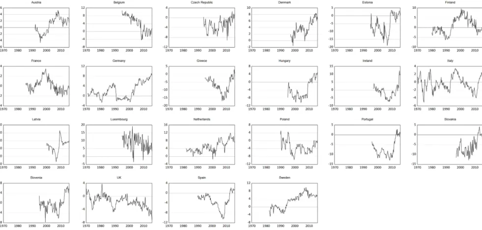
The analysis of time-series properties of current account-to-GDP ratio as well as export and import-to-GDP ratios is based on the quarterly OECD dataset. It covers a relatively large timespan (going back to 1970:Q1 for some countries)14, but some new EU countries are not considered in this dataset (Bulgaria, Croatia, Cyprus, Lithuania, Malta and Romania). Figure 1 illustrates current account balance-to-GDP ratio in the countries under scrutiny.
[Figure 1]
We can summarize the evolution of CA/GDP ratios displayed in Figure 1 as follows: there are 11 countries with CA deficits, with a deterioration or downward trend in the series (United Kingdom), an improvement or upward trend (Slovakia and Czech Republic), or no discernable trend over the whole period due to a structural break, most of the time during the recent crisis (Estonia, Greece, Hungary, Ireland, Latvia, Poland, Portugal, and Spain). There
12 Gourinchas and Rey (2007) write that "[…] we remain agnostic about the role of the exchange rate in eliminating U.S. [trade] imbalances" (p. 682). In addition, introducing the trade effects of exchange rate changes would require that we used the shares of local, producer and vehicle currencies in invoicing currency.
13 Lane and Shambaugh (2010) and Bénétrix et al. (2015) showed that most of valuation effects come from currency valuation effects.
are 3 countries with CA/GDP close to balance on average over the whole sample period (Italy, France, and Slovenia). There are 8 countries with CA surpluses, showing a downward trend (Belgium and Luxembourg), an upward trend (Denmark, Germany, the Netherlands, and Sweden) or no trend (Austria and Finland).
With regard to the second approach based on the dynamic external constraint, we use annual data from IMF databases (Balance of Payments and International Investment Position; World Economic Outlook, October 2016; International Financial Statistics) and European Commission (AMECO). Our macroeconomic variables are foreign assets, foreign liabilities, GDP, GDP deflator, trade balance, and interest rate. The sample period is 1995-2015, but for many countries, the sample is shorter due to a lack of data. Croatia is not considered because of too many missing monetary data. As mentioned in the previous section, we also use the BLS dataset for the shares of foreign assets and liabilities (in the NIIP and NED) in foreign currency and for the foreign debt assets and foreign debt liabilities. Their dataset covers the 1990-2012 period.15 There are four missing countries in their dataset: Bulgaria, Cyprus, Luxembourg and Malta. Hence, the second empirical strategy concerns 23 EU countries.
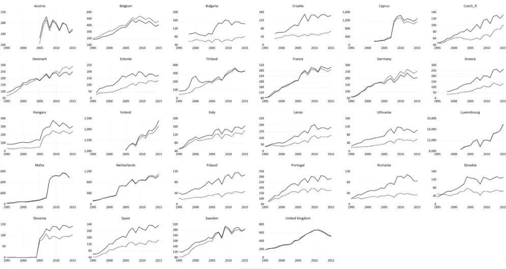
Figure 2 displays the evolution of total foreign assets and liabilities as a percentage of GDP. Broadly speaking, there are four groups of countries (in the EU): a sharp deterioration of the NIIP in Ireland16, Greece, Cyprus, and Portugal; a noticeable improvement of the NIIP in the Netherlands and Denmark (or a very slight deterioration in Sweden and Finland); a persistent positive NIIP in Belgium and Germany; and a persistent negative NIIP in most EU countries, be they old Member States (Italy) or new Member States (Poland).
[Figure 2]
15 Since we have data of the NIIP up to 2015, we take the values ofν and µ observed in 2012 for the following years 2013-2015. For the analysis of the NED, we use the BLS data, and the period ends up in 2012.
16 Ireland has a negative NIIP but its net external debt is negative (implying that the value of assets exceeds that of liabilities).
4.2. First Empirical Strategy
4.2.1 Time Series Unit Root and Cointegration Tests
In line with theoretical arguments exposed in section 3, we begin with time-series diagnostics of current account-to-GDP ratio (CA). We proceed with two standard unit root tests: augmented Dickey-Fuller, (ADF, 1979) and Phillips-Perron (PP, 1988) and one stationarity test – Kwiatkowski, Phillips, Schmidt, and Shin (KPSS, 1992). The detailed results of these tests are available on request.
There is evidence of sustainability in only eight countries according to unit root tests: three deficit countries (the Czech Republic, Poland, and Slovakia), two countries with CA close-to-balance (France and Italy), and three surplus countries (Belgium, Finland, and Luxembourg). The stationary tests confirm sustainability for Italy, Belgium and Luxembourg. Among deficit countries, sustainability is not rejected for Greece, Ireland, Latvia and Spain.
However, as accurately pointed out by Perron (1989), standard tests tend to fail to reject unit root even if a series is stationary but contains a structural break. We consider two types of structural breaks: innovational outlier, where since the break the series diverges progressively from its previous behaviour; or an additive outlier, where a sudden shift in the series occurs (Perron and Vogelsang, 1992). Results of these two types of tests are presented in Table 1. The null hypothesis is of a unit root against an alternative of stationarity with structural break.
[Table 1]
Our inference on sustainability of the CA is based on the following decision criteria: rejection of a unit root under either innovational or additive outlier with intercept only is interpreted as indicating sustainability. Rejection of a unit root in either setup under assumption of a trend is indicating sustainability only if an upward trend is detected in a deficit country or a downward trend in a surplus country.
The results indicate that the CA is sustainable in 11 countries. Among deficit countries, there are the Czech Republic, Greece (with a break in 2011Q3)17, Hungary, Latvia (break in 2008Q4), Slovakia, Portugal and the United Kingdom. Among close-to-balance countries, there is Slovenia.18 Among surplus countries, there are Belgium, Denmark (stationary with a break in the intercept under the additive outlier approach), and Luxembourg.
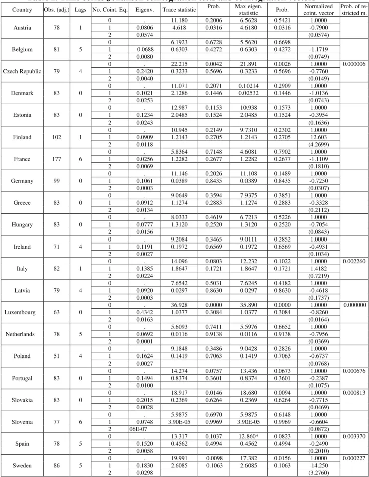
Cointegration tests as a means of assessing current account sustainability are also run. In order to inspect this further, we rely on the traditional Johansen-Juselius cointegration test. This is possible, as unit roots are present in almost all exports and imports-to-GDP series, except for the United Kingdom (results available on request).
The lag structure is selected on a basis of AIC criterion19 in a corresponding VAR model in levels. Then, cointegration tests are performed for all the countries in the sample (relying on both trace and maximum eigenvalue), except the United Kingdom. If cointegration is detected, the vector error correction model with cointegration vector restricted to (1, -1) is tested, which would be a proof of sustainability (see e.g. Quintos, 1995 or Westerlund and Prohl, 2010). The results displayed in Table 2 indicate that there is no evidence of sustainability, in spite of cointegration identified in seven countries.
[Table 2]
Overall, we can summarize the results from the various tests as follows. There is evidence of sustainability of the current account balance in eight countries. Specifically, these countries are: Belgium, Denmark (with a break in intercept), and Luxembourg, among surplus
17 The adjustment in the current account of Greece (see Figure 1) can be explained by a marked contraction in imports, a reduction in government interest payments, and transfers of profits made by national central banks on Greek bond holdings (European Commission, 2014).
18 In case of Italy we rely on standard unit root and stationarity tests because, even if test allowing for structural break fail to reject the unit root, the Bai and Perron (2003a) test indicates no break in the series.
19 The choice of AIC is robust, as in all the cases the optimal number of lags according to AIC criterion overlapped with the majority among LR, FPE, AIC, SC, and HQ.
countries; close-to-balance Italy (no break); and the Czech Republic, Greece (break in 2011Q3), Latvia (break in 2008Q4), and Slovakia among deficit countries.
4.2.2 Panel Data Unit Root and Cointegration Tests
We implement three different types of panel unit root tests: two first generation tests, namely the Im et al. (2003) test (IPS); the Maddala and Wu (1999) test (MW) and one second generation test – the Pesaran (2007) CIPS test. The latter test is associated with the fact that first generation tests do not account for cross-sectional dependence of the contemporaneous error terms, and not considering it may cause substantial size distortions in panel unit root tests (Pesaran, 2007). There has been a lot of work on testing for cross-sectional dependence in the spatial econometrics literature.20 Pesaran (2004) proposes a test (called CD test) for cross-sectional dependence using the pairwise average of the off-diagonal sample correlation coefficients in a seemingly unrelated regressions model. Results from performing the CD test on our three variables of interest reveal that the test statistic is 13.09, 98.13 and 101.91, respectively for the current account, exports and imports (not shown but available upon request). These correspond to p-values close to zero, therefore rejecting the null of cross-section independence and motivating the use of Pesaran’s (2007) CIPS test for unit roots.
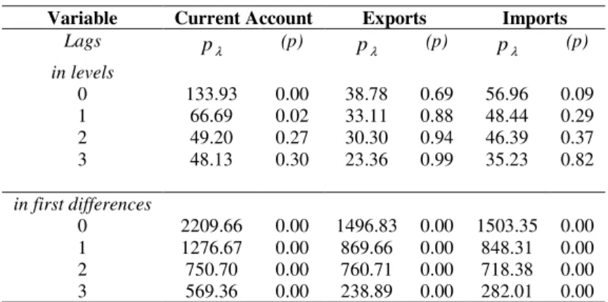
Tables 3.a and 3.b display the results of such analysis. These report the outcome for the full sample of the three panel unit root tests described above. The IPS test shows that the null hypothesis of unit roots for the panel for exports cannot be rejected when this variable is taken in levels. However, without accounting for cross-sectional dependency (which we confirm to exist in our panel), both the current account and imports seem to be stationary in levels. This is no longer true in the MW tests. When we run the CIPS that accounts for cross-sectional dependence, our previous results are strengthened particularly as lags increase. Hence, we
conclude that most conservatively: i) our panel is non-stationary and ii) cross-sectional dependence seems to play an important role.
[Tables 3.a-3.b]
We then employ a recent panel data stationarity test, which under the null hypothesis of panel stationarity takes multiple structural breaks into account (Carrion-i-Silvestre et al. (2005), CBL hereafter). The test of the null hypothesis of a stationary panel follows as recommended by CBL (2005), the estimation of the number of structural breaks and their position is based on the procedure in Bai and Perron (1998), which computes the overall minimization of the sum of the squared residuals. Following Bai and Perron (2003b) we estimate the number of structural breaks associated with each individual using the modified Schwarz information criteria.21 Applying the CBL (2005) panel data stationarity test, we find that, when we allow for cross-section dependence and when we use the bootstrap critical values (see Table 4), the null of stationarity can be rejected at usual levels by either the homogeneous or heterogeneous long-run version of the test. Overall, evidence points to non-stationarity of the three variables of interest in levels even after multiple structural breaks and cross-section dependence are allowed for.
[Table 4]
Now that panel stationarity has been covered and we found that unit roots characterize our series of interest, we proceed to inspect whether exports and imports are cointegrated within the panel. To this end, we employ a number of tests, several of them are quite recent.
First, we implement the panel cointegration tests proposed by Pedroni (2004). This is a residual-based test for the null of no cointegration in heterogeneous panels. Two classes of statistics are considered in the context of the Pedroni test. The first type is based on pooling the
21 CBL (2005) suggested that in the empirical process, the specified maximum number of structural breaks is five. We compute the finite sample critical values using Monte Carlo simulations with 20,000 replications; in other words, we approximate the empirical distribution of the panel data statistic by means of bootstrap techniques to get rid of the cross-section independence assumption.
residuals of the regression along the within-dimension of the panel, whereas the second type is based on pooling the residuals of the regression along the between-dimension of the panel. Table 5 shows the outcomes of Pedroni’s (2004) cointegration tests between exports and imports (both in percent of GDP). We use four within-group tests and three between-group tests to check whether the panel data are cointegrated.22 Results show that the null hypothesis of no cointegration can be rejected. Therefore, there exists a stable long-run relationship governing the dynamics between exports and imports for the panel of all countries in our sample.
[Table 5]
Pedroni (2004) test does not consider neither structural breaks in the cointegrating relationship nor cross-sectional dependence. Hence, the next step is to rely on the Westerlund (2007) error correction-based panel cointegration test. As shown by Banerjee, Dolado and Mestre (1998), the invalid common factor restriction in residual-based tests (such as Pedroni, 2004) can lead to severe power loss. Westerlund (2007) develops two group mean statistics and two panel statistics in order to test for null of no cointegration against two distinct alternatives such that under one of them at least one cross section is cointegrated allowing for heterogeneity and under the other one, panel is cointegrated as a whole assuming homogeneous long-run relation among the cross sections, respectively. To construct test statistics, a conditional error correction model is considered (Persyn and Westerlund, 2008). This test could be used both in existence and in non-existence of cross-sectional dependency.23 Results in Table 6 show that the null of no cointegration is rejected at the 10 percent level when cross-sectional dependencies are accounted for and this is true irrespectively of the tests under scrutiny.
22 The columns labelled within-dimension contain the computed value of the statistics based on estimators that pool the autoregressive coefficient across different countries for the unit root tests on the estimated residuals. The columns labelled between-dimension report the computed value of the statistics based on estimators that average individually calculated coefficients for each country.
23 He considers cross-sectional dependence by a bootstrap procedure and in addition, tests allow for heterogeneous short run and long run dynamics, such as heterogeneous autocorrelation structure among cross sections, individual specific intercepts, trend terms and slope coefficients and weakly exogenous regressors. Standard asymptotically normal distribution is used when cross-sectional dependency does not exist.
[Table 6]
The next test considered is the error correction-based cointegration test by Gengenbach et al. (2015), which builds on earlier work by Westerlund (2007) by augmenting the model with cross-sectional averages. The averages are then interacted with country-dummies to allow for country-specific parameters. The results of the ECM cointegration test suggested by Gengenbach, Urbain and Westerlund (2015) are reported in Table 7. The test statistic under Model 2 (which includes only a constant term) rejects the null hypothesis of no cointegration at the at the 10 percent level.
[Table 7]
Finally, we run the panel cointegration test by Banerjee and Carrion-i-Silvestre (2017). This test runs a standard CIPS panel unit root test on some sort of residuals stemming from a Pesaran (2006) CCEP model estimation. This test also controls for the dependence across the units that conform the panel using an unobserved common factor structure proxied by cross-sectional averages. This cointegration test (CADFCp) can be interpreted as a complementary examination of weak scale effects. Resulting test statisticsare displayed in Table 8. When we compare the values of the CADFCp statistic with the critical values, the null hypothesis of no cointegration is rejected in both Models 1 and 2 under zero lags at the 10 percent level of significance.
[Table 8]
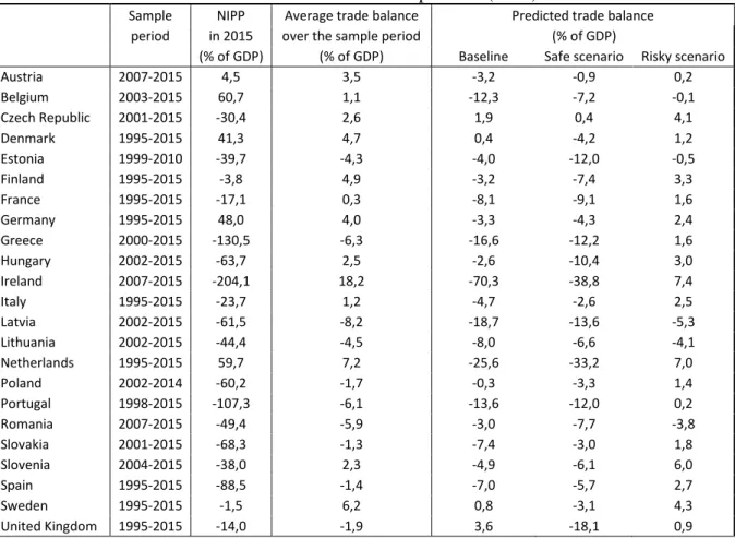
4.3. Second Empirical Strategy: Simulations
Table 9 shows the results from our second approach tackling external accounts’ sustainability. We compare the actual trade balance in percentage of GDP on average over the 1995-2015 period (or a shorter period) with the predicted trade balance that stabilizes the NFA position (NIIP or NED). The latter is based on equation (14). We made simulations under three scenarios depending on the values of parameters
ν
andµ
(the shares of foreign assets and liabilities denominated in foreign currency in total foreign assets and liabilities respectively).In the baseline scenario, we use the values retrieved from the dataset made by Bénétrix, Lane and Shambaugh (2015). In a second scenario – dubbed “safe scenario” à la Portuguese – the values of parameters for all countries and all years are those of Portugal in 2012 (in the same dataset):
ν
= 0.07 (with a weight of 4 percent for the U.S. Dollar and 2 percent for the British pound) andµ
= 0.01 (the weight of the U.S. dollar) in the NIIP, andν
= 0.04 (with a weight of 2 percent for the U.S. Dollar and 1 percent for the British pound) andµ
= 0.01 (the weight of the U.S. Dollar) in the NED. In such a case, the dynamics of the NFA is not too much influenced by valuation effects due to exchange rate movements. In a third scenario, a “risky scenario” àla British – the values of the parameters are the same as in the United Kingdom in 2012. This country is very vulnerable to any exchange rate movements. Indeed, the values are
ν
= 0.81 (with a weight of 38 percent for the U.S. Dollar inter alia) andµ
= 0.56 (with a weight of 23 percent for the U.S. Dollar) in the NIIP, andν
= 0.85 (with a weight of 42 percent for the U.S. Dollar) andµ
= 0.74 (with a weight of 30 percent for the U.S. Dollar) in the NED.24[Table 9]
According to our results, in the risky scenario, the predicted balance is often a trade surplus or close to balance, while in the safe scenario some trade deficit could be recorded without any danger of increased external indebtedness.25 Here, we draw conclusions about sustainability by taking into account three dimensions: the gap between the actual trade balance and the predicted trade balance, the position of the NIIP in the last year of the sample (2015), and its trend. We then can distinguish four categories of countries: sustainable creditors/debtors, unsustainable creditors/debtors, by looking at these three dimensions.
24 In this “British scenario”, we replace the weight of the Euro by a weight of the Pound for the EA countries. 25 A trade surplus may be required to stabilize the NIIP in some cases. We do not consider that it is an optimal trade balance. A deficit could indeed be needed for other purposes (e.g. consumption smoothing, importing capital goods, inter alia)
Overall, we can summarize the results for the NIIP as follows: the NIIP is sustainable in seven countries with a debit position (Sweden, Italy, Slovenia, the Czech Republic, Latvia, Estonia, and Hungary) and not sustainable in three countries with a credit position (Netherlands, Belgium, and Germany). There is no case of sustainability among countries with credit positions and no case of a lack of sustainability among countries with debit positions.
Concerning the net external debt, the overall picture is less rosy. Indeed, there is evidence of non-sustainable NED in two countries with a debit position (Hungary and Romania) and two countries with credit positions (Belgium and Ireland). In contrast, sustainability of the NED is found in three countries with a debit position (Czech Republic, Slovakia, and Netherlands) and no country with a credit position.
5. Conclusion and Policy Implications
Prompted notably by the thresholds of current account balance and net international investment position (NIIP) of the new Macroeconomic Imbalance Procedure (MIP) in the European Union, we carried out an analysis of external debt sustainability of EU countries. Besides, external imbalances are a greater source of concern than public deficits and debts in some countries, given their size and evolution.
We used two approaches. First, we did unit root tests of current account balance-to-GDP ratios and cointegration tests of exports and imports of goods and services. From this first assessment we can summarize the main results as follows: i) in general, the null of a unit root in the time series of current account balance-to-GDP cannot be rejected for most countries; ii) sustainability is found for Czech Republic, Slovakia, Greece and Latvia among deficit countries, Italy among close-to-balance countries, and Belgium, Luxembourg and Denmark among surplus countries; iii) the country panel is non-stationary; iv) cross-sectional dependence plays an important role; v) with multiple structural breaks and cross-sectional panel dependence
evidence points to non-stationarity of the CA, imports, and exports; vi) there is a stable long-run relationship between exports and imports for our panel.
Then, we used a dynamic external debt constraint in order to compute the trade balance that stabilizes the net foreign asset position (NIIP or net external debt) over a given period. It is fair to say that based on this analysis, there is more concern about the sustainability of external imbalances in the NIIP or NED in surplus countries than in deficit countries. Indeed, the NIIP is not sustainable in three countries with a credit position which are member countries of the Euro area (the Netherlands, Belgium, and Germany) while it is sustainable in seven countries with a debit position, of which four are member countries of the Euro area (Sweden, Italy, Slovenia, Czech Republic, Latvia, Estonia, Hungary). As for the sustainability of NED, it is found in three countries with a debit position (Czech Republic, Slovakia, Netherlands), but in no countries with credit positions. It is more of a concern (not sustainable) in two countries with debit positions (Hungary, and Romania), and two countries with credit position (Belgium and Ireland). None of these countries was the focus of the analysis of external sustainability made by the European Commission (2012b).
Overall, there is some consistency between the two approaches. Given the relationship between flows and stocks, and the existence of important structural breaks in the recent period, our first approach points to sustainability of current account-to-GDP ratio in some surplus countries (notably Belgium). On the other hand, the second approach indicates non-sustainability of their net foreign assets position (both the NIIP and the NED in the case of Belgium).26 This reinforces the case for surveillance of the evolution of external imbalances, insofar as it takes time to adjust stocks. Furthermore, due to valuation effects – via exchange rate changes in our approach – there might well be sustainable current account balances along with unsustainable net foreign asset positions. In other respects, with regard to countries with
debit net foreign asset positions, we did not find a lack of sustainability of the NIIP but of the NED for at least two countries.
Policy-wise, it would be advisable that EU policy makers could focus more on the issue of sustainability of the NED that the NIIP. Admittedly, there is a need to improve the availability of data on foreign debt assets and liabilities. They could also contemplate distinguishing between EA countries and non-EA countries in the analysis (as it is done for other indicators such as the real effective exchange rate and nominal unit labour costs in the MIP) because our results clearly show that EA countries are far less vulnerable to exchange rate valuation effects than non-EA countries.
References
1. Afonso, A. (2005). “Fiscal Sustainability: The Unpleasant European Case”, FinanzArchiv, 61(1), 19-44.
2. Afonso, A., Rault, C., Estay, C. (2013). “Budgetary and external imbalances relationship: a panel data diagnostic”, Journal of Quantitative Economics, 11(1-2), 45-71.
3. Ahmed, S., Rogers, J. (1995). “Government budget deficits and trade deficits. Are present value constraints satisfied in long-term data?” Journal of Monetary Economics, 36(2), 351-374.
4. Anselin, L., Bera, A.,(1998). “Spatial dependence in linear regression models with an introduction to spatial econometrics”. In A. Ullah and D.E.A. Giles (eds.) Handbook of Applied Economic
Statistics, 237–89. New York: Marcel Dekker.
5. Bai, J., Perron, P. (1998). “Estimating and Testing Linear Models with Multiple Structural Changes”, Econometrica, 66(1), 47-78.
6. Bai J., Perron P., (2003a). “Critical values for multiple structural change tests”, Econometrics
Journal, 6, 72-78.
7. Bai, J., Perron, P. (2003b). “Computation and Analysis of Multiple Structural Change Models”,
Journal of Applied Econometrics, 18(1), 1-22.
8. Bajo-Rubio, O., Díaz-Roldán, C., Esteve, V. (2014). “Sustainability of external imbalances in the OECD countries”, Applied Economics, 46(4), 441-449.
9. Baltagi, B.H., Song, S.H., Koh, W. (2003). “Testing panel data regression models with spatial error correlation”. Journal of Econometrics, 117, 123–150.
10. Banerjee, A. Carrion-i-Silvestre, J. L., (2017), “Testing for panel cointegration using common correlated effects estimators”, Journal of Time Series Analysis, 38(4), 610–636.
11. Banerjee, A., Dolado, J., Mestre, R., (1998). “Error-correction mechanism tests for cointegration in a single-equation framework”. Journal of Time Series Analysis, 19: 267–283.
12. Bénassy-Quéré, A. (2016). “Euro-Area Fiscal Stance: From Theory to Practical Implementation”,
CESIfo WP 6040.
13. Bénétrix, A., Lane, P., Shambaugh, J. (2015). “International currency exposures, valuation effects and the global financial crisis”, Journal of International Economics, 96, 98-109.
14. Bohn, H. (2007). “Are Stationarity and Cointegration Restrictions Really Necessary for the Intertemporal Budget Constraint?”, Journal of Monetary Economics, 54, 1837-1847.
15. Camarero, M., Carrion-i-Silvestre, J.L., Tamarit, C. (2013). “Global imbalances and the intertemporal external budget constraint: A multi-cointegration approach”, Journal of Banking and
Finance, 37, 5357-5372.
16. Camarero, M., Carrion-i-Silvestre, J.L., Tamarit, C. (2015). “Testing for external sustainability under a monetary integration process. Does the Lawson doctrine apply to Europe?”, Economic
Modelling, 44, 343-349.
17. Carrion-i-Silvestre, J. L, Barrio-Castro, T., López-Bazo, E. (2005). “Breaking the panels: An application to the GDP per capita”. Econometrics Journal, 8, 159–75.
18. Chen, S.-W. (2011). “Current account deficits and sustainability: Evidence from the OECD countries”, Economic Modelling, 28, 1455-1464.
19. Chen, S.-W. (2014), “Smooth transition, non-linearity and current account sustainability: Evidence from the European countries”. Economic Modelling, 38, 541-554.
20. Chortareas, G.E., Kapetanios, G., Uctum, M. (2004). “An Investigation of Current Account Solvency in Latin America Using Non Linear Nonstationarity Tests”, Studies in Nonlinear
21. Corsetti, G., Pesenti, P., Roubini, N. (1999). “What caused the Asian Currency and Financial Crisis?”, Japan and the World Economy, 11(3), 305-373.
22. Dickey, D. A., Fuller, W. A. (1979). “Distribution of the estimators for autoregressive time series with a unit root”, Journal of the American Statistical Association, 74(366a), 427-431.
23. Durdu, B., Mendoza, E., Terrones, M. (2013). “On the solvency of nations: Cross-country evidence on the dynamics of external adjustment”, Journal of International Money and Finance, 32,
762-780.
24. Edwards, S. (2005). “Is the US Current Account Deficit Sustainable? And If Not, How Costly is Adjustment Likely To Be?” Brookings Papers on Economic Activity, 1.
25. Eichengreen, B., Haussmann, R., Panizza, U. (2003). “Currency mismatches, debt intolerance and original sin: why they are not the same and why it matters”, NBER Working Papers 10036.
26. European Commission (2012a). “Scoreboard for the surveillance of macroeconomic imbalances”,
European Economy Occasional Papers 92, February.
27. European Commission (2012b). “The dynamics of international investment positions”, Quarterly
Report on the Euro Area, No. 3.
28. European Commission (2014). “The Second Economic Adjustment Programme for Greece – Fourth Review”, European Economy, Occasional Papers 192, April.
29. Gengenbach, C., Urbain, J.-P., Westerlund, J. (2015), “Error Correction Testing in Panels with Common Stochastic Trends”, Journal of Applied Econometrics, 311(6), 982-1004.
30. Gourinchas, P.-O., Rey, H. (2007). “International Financial Adjustment”, Journal of Political
Economy, 115(4), 665-703.
31. Hakkio, G., Rush, M. (1991). “Is the budget deficit "too large?"” Economic Inquiry, 29(3), 429-445. 32. Holmes, M. (2006), “How sustainable are OECD current account balances in the long run?”,
Manchester School, 74(5), 626-643.
33. Im, K. S., Pesaran, M. H. Shin, Y. (2003), “Testing for unit roots in heterogeneous panels”, Journal
34. Kim, D., Perron P. (2009). “Unit Root Tests Allowing for a Break in the Trend Function at an Unknown Time Under Both the Null and Alternative Hypotheses”, Journal of Econometrics, 148,
1–13.
35. Kwiatkowski, D., Phillips, P. C., Schmidt, P., Shin, Y. (1992). “Testing the null hypothesis of stationarity against the alternative of a unit root: How sure are we that economic time series have a
unit root?”, Journal of Econometrics, 54(1-3), 159-178.
36. Lane, P., Milesi-Ferretti, G. (2007). “Europe and global imbalances”, Economic Policy, 22(51), 519-573.
37. Lane, P., Shambaugh, J. (2010). “Financial Exchange Rates and International Currency Exposures”,
American Economic Review, 100(1), 518-540.
38. Maddala, G. S., Wu, S. (1999). “A Comparative Study of Unit Root Tests with Panel Data and New Simple Test", Oxford Bulletin of Economics and Statistics, 61, 631-652
39. Milesi-Ferretti, G.M., Razin, A. (1996). “Current-Account Sustainability”, NBER Working Paper 81.
40. Obstfeld, M., Rogoff, K. (2005). “Global current account imbalances and exchange rate adjustments”, Brookings Papers on Economic Activity, 1, 67-146.
41. Pedroni, P. (2004), “Panel Cointegration; Asymptotic and Finite Sample Properties of Pooled Time series Tests, With an Application to the PPP Hypothesis,” Econometric Theory, 20, 597-625.
42. Pedroni, P. (1999), “Critical Values for Cointegration Tests in Heterogeneous Panels with Multiple Regressors", Oxford Bulletin of Economics and Statistics, 61, 653-670.
43. Perron, P. (1989). “The great crash, the oil price shock, and the unit root hypothesis”, Econometrica:
Journal of the Econometric Society, 1361-1401.
44. Perron, P., Vogelsang, T. J. (1992). “Nonstationarity and level shifts with an application to purchasing power parity”, Journal of Business & Economic Statistics, 10(3), 301-320.
45. Persyn, D. Westerlund, J., (2008). “Error Correction Based Cointegration Tests for Panel Data”.
Stata Journal 8 (2), 232-241.
46. Pesaran, M.H. (2004), "General Diagnostic Tests for Cross Section Dependence in Panels", CESifo
47. Pesaran, M.H., (2007), “A simple panel unit root test in the presence of cross section dependence”,
Journal of Applied Econometrics, 22, 265-312.
48. Phillips, P. C., Perron, P. (1988). “Testing for a unit root in time series regression”, Biometrika, 75(2), 335-346.
49. Quintos, C. (1995). “Sustainability of the Deficit Process with Structural Shifts,” Journal of
Business and Economic Statistics, 13(4), 409-417.
50. Raybaudi, M., Sola, M., Spagnolo, F. (2004). “Red Signals: Current Account Deficits and Sustainability,” Economics Letters, 84(2), 217-223.
51. Trehan, B., Walsh, C. (1991). “Testing Intertemporal Budget Constraints: Theory and Applications to U.S. Federal Budget and Current Account Deficits,” Journal of Money, Credit, and Banking,
23(2), 206-223.
52. Vogelsang, T., Perron, P. (1998). “Additional Test for Unit Root Allowing for a Break in the Trend Function at an Unknown Time,” International Economic Review, 39, 1073–1100.
53. Westerlund, J. (2007). “Testing for error correction in panel data”. Oxford Bulletin of Economics
and Statistics 69: 709–748.
54. Westerlund, J., Prohl, S. (2010). “Panel Cointegration Tests of the Sustainability Hypothesis in Rich OECD Countries”, Applied Economics, 42, 1355-1364.
Figure 1. Current Account-to-GDP ratio
Figure 2. Foreign Assets and Liabilities (percentage of GDP)
Table 1. Results of unit root tests of the CA-to-GDP ratio with endogenously determined structural break
Country Sample period
Innovation outlier Additive outlier Intercept Trend and intercept,
break in intercept
Trend and intercept,
break in both Intercept
Trend and intercept, break in intercept
Trend and intercept, break in both Break t-Stat Prob. Break t-Stat Prob. Break t-Stat Prob. Break t-Stat. Prob. Break t-Stat Prob. Break t-Stat. Prob. Austria 1992Q1-2015Q4 2001Q2 -3.7607 0.2530 2001Q2 -3.5611 0.6547 2001Q2 -3.1775 0.9302 2000Q4 -4.2505 0.0850 2000Q4 -4.0922 0.3166 2000Q4 -3.6643 0.7305 Belgium 1995Q1-2015Q4 2007Q3 -5.3338 < 0.01 2008Q1 -7.8117 < 0.01 2008Q1 -7.8117 < 0.01 2005Q2 -4.8182 0.0168 2005Q2 -5.4945 < 0.01 2008Q3 -5.7905 < 0.01 Czech Rep. 1994Q1-2015Q4 2013Q1 -3.9710 0.1656 2002Q1 -5.3310 0.0109 2001Q4 -5.2723 0.0388 2004Q3 -6.2519 < 0.01 2000Q1 -6.7270 < 0.01 2003Q4 -6.7834 < 0.01 Denmark 1997Q1-2015Q4 2009Q4 -3.5288 0.3711 2006Q1 -6.2907 < 0.01 2006Q1 -6.5932 < 0.01 2010Q2 -4.4813 0.0455 2005Q3 -6.1959 < 0.01 2007Q1 -6.3042 < 0.01 Estonia 1995Q1-2015Q4 2008Q3 -4.3688 0.0616 2008Q3 -4.7831 0.0620 2008Q3 -4.5265 0.2256 2007Q4 -3.9481 0.1738 2008Q1 -4.4242 0.1586 2005Q1 -4.5350 0.2215 Finland 1980Q1-2015Q4 1992Q2 -2.6348 0.8566 1993Q1 -4.0546 0.3380 1993Q1 -4.0402 0.4944 1991Q4 -2.6434 0.8530 1993Q4 -3.8565 0.4641 1992Q3 -3.9092 0.5815 France 1985Q3-2015Q4 2001Q3 -2.1665 0.9670 2002Q4 -2.7796 0.9571 2001Q4 -3.4917 0.8167 1998Q4 -2.2589 0.9537 2003Q1 -2.8502 0.9465 2001Q4 -3.0150 0.9599 Germany 1971Q1-2015Q4 2003Q2 -3.3442 0.4774 1990Q1 -4.1483 0.2876 1990Q1 -4.8813 0.1033 2003Q2 -3.3649 0.4635 2003Q2 -3.4326 0.7319 1991Q1 -3.4994 0.8129 Greece 1995Q1-2015Q4 2011Q3 -2.2091 0.9617 2011Q3 -3.3175 0.7937 2006Q4 -7.0217 < 0.01 2011Q2 -2.4683 0.9107 2011Q3 -5.2282 0.0162 2006Q4 -7.1371 < 0.01 Hungary 1995Q1-2015Q4 2008Q4 -4.7712 0.0193 2008Q4 -4.9989 0.0333 2008Q4 -5.6602 0.0128 2008Q4 -4.8097 0.0173 2008Q4 -5.0235 0.0308 2008Q4 -5.6856 0.0116 Ireland 1997Q1-2015Q4 2014Q2 -2.8339 0.7710 2012Q4 -3.2570 0.8220 2006Q4 -4.2567 0.3606 2012Q1 -2.4947 0.9043 2012Q2 -2.9206 0.9332 2006Q4 -4.4239 0.2733 Italy 1970Q1-2015Q4 2012Q1 -3.5344 0.3682 1992Q3 -3.6620 0.5893 2007Q3 -3.9430 0.5606 2012Q1 -3.5575 0.3553 1992Q3 -3.6978 0.5658 2007Q3 -3.9744 0.5396 Latvia 2000Q1-2015Q4 2008Q4 -3.8577 0.2110 2008Q4 -5.4220 < 0.01 2008Q4 -6.0016 < 0.01 2006Q1 -3.4766 0.4001 2009Q3 -3.4643 0.7144 2007Q2 -3.9519 0.5547 Luxembourg 1995Q1-2015Q4 2008Q3 -8.4302 < 0.01 2003Q1 -9.4019 < 0.01 2003Q1 -9.3622 < 0.01 2008Q1 -8.5141 < 0.01 2003Q2 -9.1936 < 0.01 2003Q2 -9.1850 < 0.01 Netherlands 1982Q1-2015Q4 2003Q1 -4.2796 0.0782 2009Q1 -5.4099 < 0.01 1999Q2 -5.6133 0.0150 2002Q1 -4.2964 0.0753 2006Q1 -5.2416 0.0155 1996Q3 -5.2231 0.0444 Poland 1990Q1-2015Q4 1995Q4 -4.2398 0.0877 1995Q4 -4.6979 0.0777 1996Q3 -4.6781 0.1644 1995Q4 -4.2752 0.0790 1996Q4 -4.7617 0.0656 1995Q4 -4.7667 0.1344 Portugal 1996Q1-2015Q4 2011Q2 -4.5466 0.0381 2011Q2 -4.5273 0.1221 2007Q3 -4.8983 0.0989 2011Q3 -2.9012 0.7384 2011Q3 -3.4563 0.7199 2006Q3 -4.2162 0.3843 Slovakia 1997Q1-2015Q4 2011Q3 -4.0846 0.1292 2001Q2 -5.5976 < 0.01 2003Q3 -5.5360 0.0186 2011Q3 -5.4159 < 0.01 2000Q3 -6.0774 < 0.01 2000Q3 -6.3164 < 0.01 Slovenia 1995Q1-2015Q4 2012Q1 -3.9117 0.1889 2012Q1 -3.9697 0.3911 2007Q1 -5.1537 0.0534 2012Q2 -5.6410 < 0.01 2012Q2 -5.6242 < 0.01 2007Q1 -6.8545 < 0.01 Spain 1990Q1-2015Q4 2011Q4 -2.0445 0.9802 2008Q4 -3.2518 0.8241 2004Q1 -3.9159 0.5772 2009Q3 -2.1796 0.9654 2009Q3 -2.6687 0.9703 2004Q1 -3.9030 0.5861 Sweden 1982Q1-2015Q4 1993Q1 -3.7401 0.2626 2011Q3 -3.6665 0.5863 2002Q4 -3.9908 0.5276 1992Q1 -3.6414 0.3111 2008Q3 -3.1794 0.8527 2000Q1 -3.6846 0.7170 UK 1970Q1-2015Q4 2011Q2 -3.3486 0.4744 2011Q2 -3.6009 0.6287 2009Q1 -3.6037 0.7646 2012Q2 -4.7406 0.0214 2012Q1 -5.3358 0.0106 2012Q1 -5.4169 0.0262
Notes: Denote BC DE as the intercept break variable, BD DE as the trend break variable, B DE as one-time break variable, F as the CA-to-GDP ratio, G as a lag polynomial and H as IID innovations. The innovation outlier specification tests the null of F = F + I1 + G JBC DE + 4BD DE + H , against the alternative hypotheses which are nested in a general Dickey-Fuller test equation of F = + I1 + JBC DE + 4BD DE + KB DE + LF + ∑ MONP NΔF N+ R . The t-statistic is used for comparing LS to 1 (1TU) to evaluate the null hypothesis. The “intercept” model sets I = 4 = 0, the “trend and intercept, break in intercept” model sets 4 = 0, the trend and intercept, break in both
leaves the test equation unrestricted. The additive outlier tests the null of F = F + I1 + JB DE + 4BC DE + G H against a general alternative of F = + I1 + JBC DE + 4BD DE + G H . In a two-step procedure the model is first adequately detrended and then the Dickey-Fuller test is performed. See Vogelsang and Perron (1998) and Kim and Perron (2009) for discussion. Optimal lag length is chosen according to Akaike information criterion and selected break minimizes Dickey-Fuller t-statistics.
Table 2. Time-series Johansen cointegration tests and cointegration vectors Country Obs. (adj.) Lags No. Coint. Eq. Eigenv. Trace statistic Prob. Max eigen.
statistic Prob. Normalized coint. vector Prob. of re-stricted m. Austria 78 1 0 . 11.180 0.2006 6.5628 0.5421 1.0000 1 0.0806 4.618 0.0316 4.6180 0.0316 -0.7900 2 0.0574 (0.0574) Belgium 81 5 0 6.1923 0.6728 5.5620 0.6698 1 0.0688 0.6303 0.4272 0.6303 0.4272 -1.1719 2 0.0080 (0.0749) Czech Republic 79 4 0 . 22.215 0.0042 21.891 0.0026 1.0000 0.000006 1 0.2420 0.3233 0.5696 0.3233 0.5696 -0.7760 2 0.0040 (0.0149) Denmark 83 0 0 . 11.071 0.2071 0.10214 0.2909 1.0000 1 0.1021 2.1286 0.1446 0.02532 0.1446 -1.0136 2 0.0253 (0.0743) Estonia 83 0 0 . 12.987 0.1153 10.938 0.1573 1.0000 1 0.1234 2.0485 0.1524 2.0485 0.1524 -0.3954 2 0.0243 (0.1636) Finland 102 1 0 . 10.945 0.2149 9.7310 0.2302 1.0000 1 0.0909 1.2143 0.2705 1.2143 0.2705 12.603 2 0.0118 (4.2699) France 177 6 0 . 5.8364 0.7148 4.6081 0.7902 1.0000 1 0.0256 1.2282 0.2677 1.2282 0.2677 -1.1109 2 0.0069 (0.1810) Germany 99 0 0 . 11.146 0.2026 11.108 0.1489 1.0000 1 0.1061 0.0389 0.8435 0.0389 0.8435 -0.7250 2 0.0003 (0.0307) Greece 83 0 0 . 9.0649 0.3594 7.9375 0.3851 1.0000 1 0.0912 1.1274 0.2883 1.1274 0.2883 -0.3328 2 0.0134 (0.2112) Hungary 83 0 0 . 8.0333 0.4619 6.7213 0.5226 1.0000 1 0.0777 1.3120 0.2520 1.3120 0.2520 -0.7054 2 0.0156 (0.0843) Ireland 71 4 0 . 9.2084 0.3465 9.0111 0.2852 1.0000 1 0.1191 0.1972 0.6569 0.1972 0.6569 -0.4931 2 0.0027 (0.1034) Italy 82 1 0 . 14.096 0.0803 12.232 0.1022 1.0000 0.002260 1 0.1385 1.8647 0.1721 1.8647 0.1721 1.4182 2 0.0224 (0.7219) Latvia 79 4 0 . 7.6542 0.5031 7.6245 0.4182 1.0000 1 0.0920 0.0297 0.8630 0.0297 0.8630 -0.4618 2 0.0003 (0.1737) Luxembourg 63 0 0 . 36.928 0.0000 35.890 0.0000 1.0000 0.000000 1 0.4342 1.0377 0.3084 1.0377 0.3084 -0.8260 2 0.0163 (0.0164) Netherlands 78 5 0 . 5.6093 0.7411 5.5976 0.6652 1.0000 1 0.0692 0.0116 0.9138 0.0116 0.9138 -0.7956 2 0.0001 (0.0369) Poland 51 4 0 . 9.1848 0.3486 9.0428 0.2826 1.0000 1 0.1624 0.1419 0.7063 0.1419 0.7063 -0.6737 2 0.0027 (0.0768) Portugal 83 0 0 . 14.274 0.0757 13.436 0.0673 1.0000 0.000676 1 0.1494 0.8374 0.3601 0.8374 0.3601 -0.2387 2 0.0100 (0.1075) Slovakia 83 0 0 . 18.917 0.0146 18.680 0.0094 1.0000 0.000813 1 0.2015 0.2369 0.6264 0.2369 0.6264 -0.7715 2 0.0028 (0.0469) Slovenia 77 6 0 . 5.9875 0.6970 5.9875 0.6148 1.0000 1 0.0748 3.90E-05 0.9969 3.90E-05 0.9969 -0.6604 2 5.06E-07 (0.0872) Spain 78 5 0 . 13.317 0.1037 12.860* 0.0823 1.0000 0.003370 1 0.1520 0.4562 0.4994 0.4562 0.4994 -0.2490 2 0.0058 (0.2010) Sweden 86 5 0 . 19.991 0.0098 17.382 0.0156 1.0000 0.000227 1 0.1830 2.6085 0.1063 2.6085 0.1063 -14.250 2 0.0298 (3.2760)
Note: the critical values at 5% significance level for trace statistics are: 15.41 rejecting the null of no cointegration and and 3.76 rejecting at most 1 cointegrating relation. For max eigenvalue statistics these are, respectively 14.07 and 3.76