www.biogeosciences.net/11/3015/2014/ doi:10.5194/bg-11-3015-2014
© Author(s) 2014. CC Attribution 3.0 License.
Using biogeochemical data assimilation to assess the relative skill of
multiple ecosystem models in the Mid-Atlantic Bight: effects of
increasing the complexity of the planktonic food web
Y. Xiao and M. A. M. Friedrichs
Virginia Institute of Marine Science, College of William & Mary, P.O. Box 1346, Gloucester Point, VA 23062, USA
Correspondence to:M. A. M. Friedrichs ([email protected])
Received: 8 December 2013 – Published in Biogeosciences Discuss.: 8 January 2014 Revised: 4 April 2014 – Accepted: 20 April 2014 – Published: 6 June 2014
Abstract.Now that regional circulation patterns can be rea-sonably well reproduced by ocean circulation models, sig-nificant effort is being directed toward incorporating com-plex food webs into these models, many of which now rou-tinely include multiple phytoplankton (P) and zooplankton (Z) compartments. This study quantitatively assesses how the number of phytoplankton and zooplankton compartments af-fects the ability of a lower-trophic-level ecosystem model to reproduce and predict observed patterns in surface chloro-phyll and particulate organic carbon. Five ecosystem model variants are implemented in a one-dimensional assimilative (variational adjoint) model testbed in the Mid-Atlantic Bight. The five models are identical except for variations in the level of complexity included in the lower trophic levels, which range from a simple 1P1Z food web to a considerably more complex 3P2Z food web. The five models assimilated satellite-derived chlorophyll and particulate organic carbon concentrations at four continental shelf sites, and the result-ing optimal parameters were tested at five independent sites in a cross-validation experiment. Although all five models showed improvements in model–data misfits after assimila-tion, overall the moderately complex 2P2Z model was asso-ciated with the highest model skill. Additional experiments were conducted in which 20 % random noise was added to the satellite data prior to assimilation. The 1P and 2P models successfully reproduced nearly identical optimal parameters regardless of whether or not noise was added to the assimi-lated data, suggesting that random noise inherent in satellite-derived data does not pose a significant problem to the as-similation of satellite data into these models. However, the most complex model tested (3P2Z) was sensitive to the level of random noise added to the data prior to assimilation,
high-lighting the potential danger of over-tuning inherent in such complex models.
1 Introduction
2007) revealed that ecosystem models with multiple phyto-plankton (P) state variables were quantitatively more skill-ful (in terms of reproducing observations of chlorophyll, pri-mary production, export and nitrate at multiple sites) than models with single P compartments. However, the 12 mod-els participating in the Friedrichs et al. (2007) comparison study varied in many different ways, including nutrient limi-tations, variable elemental compositions and zooplankton (Z) state variables, making it difficult to determine why certain models performed better than others. Lehmann et al. (2009) compared two models with different numbers of plankton compartments (1P1Z with 2P1Z) and concluded that the ad-ditional phytoplankton state variable improved model skill. However, in this case it was not completely clear whether the improvement was due to the additional phytoplankton com-partment or was caused by other differences in the structures of the two models such as the variable carbon : nitrogen ra-tio included in the more complex model. Likewise, Hash-ioka et al. (2012) evaluated the role of functional groups in four global ecosystem models. Although differences in model performance were found, these were largely attributed to variations in underlying governing mechanisms, and not necessarily to differences in the numbers and specific char-acteristics of each model’s phytoplankton functional types.
In contrast to these previous efforts that compared mod-els that varied in many ways based on different assumptions made by different investigators, Bagniewski et al. (2011) compared the relative skill of three models that differed only in their formulations for fast-sinking diatom aggregates and cysts. Although none of their models could be rejected based on misfit with available observations, the inclusion of export by diatom aggregation was found to be a process that signif-icantly improved model–data fit. In the study presented here, the focus is on the inter-model differences induced solely by variations in the assumed phytoplankton and zooplankton structures. In other words, the five ecosystem models tested in this study are identical except for variations in the level of complexity included in the P and Z compartments, and range from a simple 1P1Z to a considerably more complex 3P2Z food web. To further simplify the comparison, func-tional types were not considered, but instead, the multiple P and Z only account for size class differences.
Here relative model skill is defined as how well the models represent observations over a specified range of conditions, or, more practically, how well the models fit the data (Jolliff et al., 2009; Stow et al., 2009, Friedrichs et al., 2009). Since ecosystem model performance is very sensitive to the arbi-trary choice of ecological parameter values (Rykiel, 1996), it is critical to rigorously optimize the parameter values of individual models prior to comparing their relative skill in order to insure that innate differences in model structures are being compared, rather than the degree of subjective tuning (Friedrichs et al., 2006). Thus in this analysis each of the five models was parameterized in a 1-D assimilative framework, and parameters were optimized through the assimilation of
satellite-derived data. In this way, all five models were com-pared at their optimum skill. In addition, because all models were forced with identical physics, the difference in model performance was only a function of the varying P and Z food web structures.
The objective of this study is not to identify a model with the highest possible skill in this particular region of the ocean, but rather the goal is to determine how varying the number of plankton variables within a given model af-fects model performance. In other words, this study exam-ines how model skill, specifically skill in reproducing surface chlorophyll and particulate organic carbon concentrations, is affected by manipulating the complexity of the planktonic food web without altering other underlying formulations and assumptions in the model.
2 Methods
2.1 Ecosystem models
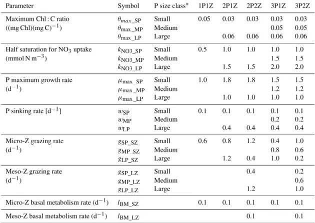
In this study five nitrogen-based marine ecosystem mod-els were compared. All are nitrogen–phytoplankton– zooplankton–detritus (NPZD)-type models incorporating identical biogeochemical processes (as described in Fennel et al. 2006), with the only difference between models be-ing the number of phytoplankton and zooplankton groups: 1P1Z, 2P1Z, 2P2Z and 3P1Z and 3P2Z food webs. The most complex 3P2Z model includes three P compartments (pico-, nano- and micro-phytoplankton) with three corresponding chlorophyll state variables and two Z compartments (micro-and meso-zooplankton). In the simplest 1P1Z model, the sin-gle P and Z compartments represent an average of three phy-toplankton size classes and micro-zooplankton, respectively. In the 2P models, one phytoplankton compartment represents the micro-phytoplankton and one represents an average of pico- plus nano-phytoplankton. The key parameters that dif-ferentiate P size classes include maximum chlorophyll-to-carbon ratios, nutrient half-saturation constants, maximum growth rates and sinking rates, whereas Z compartments vary in grazing rates and food preference. Both micro- and meso-zooplankton were assumed to graze on all phytoplank-ton size classes but with varying grazing rates. This allowed micro-zooplankton to prefer pico- and nano-phytoplankton, whereas meso-zooplankton preferred micro-phytoplankton. A summarized list of critical parameters for the various plankton state variables is provided in Table 1 and the bio-logical equations are provided in the Appendix.
Each of the five marine ecosystem models were embedded in a 1-D (vertical) physical model that contains standard pa-rameterizations for vertical advection, diffusion and sinking particles that have been thoroughly described in a number of other 1-D modeling studies (Friedrichs et al., 2007; Ward et al., 2010; Xiao and Friedrichs, 2014). Initial and bottom boundary conditions for the model state variables were set
Table 1.Key parameters that differentiate the phytoplankton (P) and zooplankton (Z) size classes.
Parameter Symbol P size class∗ 1P1Z 2P1Z 2P2Z 3P1Z 3P2Z Maximum Chl : C ratio θmax_SP Small 0.05 0.03 0.03 0.03 0.03 ((mg Chl)(mg C)−1) θmax _MP Medium 0.05 0.05
θmax _LP Large 0.06 0.06 0.06 0.06
Half saturation for NO3uptake kNO3_SP Small 0.5 1.0 1.0 1.0 1.0 (mmol N m−3) kNO3_MP Medium 1.5 1.5
kNO3_LP Large 1.5 1.5 2.0 2.0
P maximum growth rate µmax _SP Small 1.0 1.8 1.8 1.5 1.5
(d−1) µmax _MP Medium 1.2 1.2
µmax _LP Large 1.0 1.0 1.0 1.0
P sinking rate [d−1] wSP Small 0.1 0.1 0.1 0.1 0.1
wMP Medium 0.2 0.2
wLP Large 0.4 0.4 0.4 0.4
Micro-Z grazing rate gSP_SZ Small 0.6 0.8 1.2 0.4 1.0
(d−1) gMP_SZ Medium 0.8 0.6
gLP_SZ Large 1.2 0.4 1.0 0.2
Meso-Z grazing rate gSP_LZ Small 0.4 0.2
(d−1) gMP_LZ Medium 0.6
gLP_LZ Large 1.2 1.0
Micro-Z basal metabolism rate (d−1) lBM_SZ 0.1 0.1 0.1 0.1 0.1 Meso-Z basal metabolism rate (d−1) lBM_LZ 0.1 0.1
∗The three size classes represent pico-, nano- and micro-phytoplankton (small, medium and large).
the same as in Xiao and Friedrichs (2014), i.e., provided by a corresponding three-dimensional (3-D) 1P1Z model imple-mentation (Hofmann et al., 2008; 2011). Models with two size classes were initialized as one-half of the 3-D 1P1Z con-centrations, and models with three size classes were initial-ized as one-third of these concentrations. Sensitivity experi-ments demonstrated that the 1-D models were not sensitive to these initial size fractionation ratios. In all experiments, carbon was derived by converting nitrogen (N) to carbon (C) via a constant Redfield C : N ratio and model estimates of particulate organic carbon (POC) were computed as the sum of all phytoplankton, zooplankton and detritus. All five mod-els were run from 1 January 2004 through 31 December 2004 with a time step of 1 h.
2.2 Satellite-derived data
Based on the results of Xiao and Friedrichs (2014), three types of daily 9km data were derived from the Sea-viewing Wide Field-of-view Sensor (SeaWiFS) and assimilated into the five models described above (Table 2): size-fractionated chlorophyll a (Pan et al., 2010), total chlorophylla (com-puted as the sum of the size-fractionated chlorophyll) and particulate organic carbon (Stramska and Stramski, 2005). Although these satellite data were all derived using empir-ical or semi-analytempir-ical algorithms, they have demonstrated
considerable success in their agreement with in situ data. The uncertainty associated with these size-differentiated chloro-phyll and POC concentrations has been estimated to be 35 % (Pan et al., 2010; Stramska and Stramski, 2005).
Satellite-derived size-fractionated chlorophyll consists of three types of size-fractionated chlorophyll: large phyll (ChlL), medium chlorophyll (ChlM) and small chloro-phyll (ChlS), representing chlorochloro-phyll produced by micro-phytoplankton, nano-phytoplankton and pico-micro-phytoplankton, respectively. When comparing the models with two phy-toplankton components to these satellite data, the chloro-phyll attributed to the large phytoplankton component was compared to ChlL, and the chlorophyll attributed to the small phytoplankton component was compared to the sum of ChlS + ChlM. When comparing the model with one phy-toplankton component to these satellite data, the modeled chlorophyll was compared to the sum of all three types of chlorophyll.
2.3 Data assimilation framework
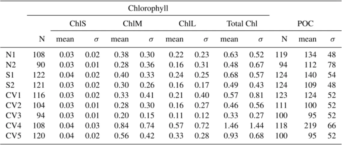
Table 2.Number of observations (N), mean and standard deviation (σ) of the satellite-derived chlorophyll concentrations (small, medium, large and total; mg Chl m−3)and POC data (mg C m−3)at each site.
Chlorophyll
ChlS ChlM ChlL Total Chl POC
N mean σ mean σ mean σ mean σ N mean σ
N1 108 0.03 0.02 0.38 0.30 0.22 0.23 0.63 0.52 119 134 48 N2 90 0.03 0.01 0.28 0.36 0.16 0.31 0.48 0.67 94 112 78 S1 122 0.04 0.02 0.40 0.33 0.24 0.25 0.68 0.57 124 140 54 S2 121 0.03 0.02 0.30 0.26 0.16 0.17 0.49 0.43 124 109 48 CV1 116 0.03 0.02 0.33 0.41 0.21 0.40 0.57 0.81 123 124 52 CV2 104 0.03 0.01 0.28 0.30 0.16 0.27 0.46 0.56 111 100 52 CV3 94 0.03 0.01 0.20 0.15 0.11 0.12 0.33 0.27 100 95 52 CV4 108 0.04 0.03 0.84 0.74 0.57 0.72 1.46 1.44 118 219 66 CV5 120 0.04 0.02 0.56 0.42 0.33 0.28 0.93 0.68 100 95 52
The variational adjoint method is a nonlinear, weighted least-squares optimization method that minimizes the misfit between the model estimates and the observational data by optimizing a subset of model parameters (e.g., Lawson et al., 1995, 1996). The choice of parameters for optimization de-pends strongly on the data available for optimization. When size-differentiated chlorophyll and particulate organic car-bon data are available for assimilation, Xiao and Friedrichs (2014) determined that successful assimilation results are ob-tained as long as data from multiple sites are assimilated, and the subset of parameters to be optimized includes max-imum chlorophyll : carbon (Chl : C) ratios, maxmax-imum phy-toplankton growth rates and zooplankton basal metabolism rates. Because each optimized parameter is size specific (that is, each phytoplankton size class has a distinct Chl : C ratio and growth rate) and each zooplankton size class has a dis-tinct basal metabolism rate (Table 1), the number of opti-mized parameters increases with increasing model complex-ity. For the five models tested here, 3, 5, 6, 7 and 8 parameters are optimized, respectively.
In this methodology the model–data misfit, otherwise known as the “cost function” (J), is minimized, where
J = 1 M
K
X
k=1 M
X
m=1 1 Nkm·σkm2
Nkm
X
j=1
(aj km− ˆaj km)2, (1)
wherea represents the modeled equivalents to the observa-tions (aˆ);Mis the number of data types, for whichM=2, 3 or 4 depending on the number of P size classes resolved by the model;K is the number of sites;Nkmis the number of
observations at sitekfor data typem; andσkmis the standard
deviation of theNkmobservations (Table 2). In this way, the
cost function provides an estimate of the ratio between the model–data differences and the differences between the data and the mean of the data, i.e.,σkm2 .
After the cost function is computed from an a priori for-ward model run, the adjoint code (Giering and Kaminski,
1998) computes the gradients of the cost function and passes the information to an optimization procedure (Gilbert and Lemaréchal, 1989), which determines how each optimized parameter value should be modified in order to reduce the magnitude of the cost function. The new parameter values are then used in another forward model run, the new cost func-tion is computed, and the optimizafunc-tion procedure is repeated. These iterations continue until the specified convergence cri-terion is satisfied.
Following the recommendations of Xiao and Friedrichs (2014), both particulate organic carbon and size-differentiated chlorophyll were assimilated. Although this previous study found that POC estimates were not sig-nificantly improved as a result of the assimilation, the POC assimilation played a critical role in preventing significant deterioration of other state variables (zooplankton, detritus) that are included as components of POC. Thus the cost that was minimized by the optimization routine consists of the sum of these two components:
Size_cost=SizeChl_cost+POC_cost, (2) where SizeChl_cost represents that portion of the cost due to the model–data misfits of size-differentiated chlorophyll, and POC_cost represents the portion of the cost due to the POC model–data misfits. For the 1P model, SizeChl_cost is computed for total chlorophyll (ChlS + ChlM + ChlL) and thus M=2 in Eq. (1) (i.e., one data type is total ChlS + ChlM + ChlL and one is POC.) For the 2P models, SizeChl_cost is computed as the sum of two separate com-ponents: ChlS + ChlM and ChlL. In this case M=3 (data types are ChlS + ChlM, ChlL and POC.) Finally, for the 3P models, SizeChl_cost includes misfits for ChlS, ChlM and ChlL separately, and four data types are assimilated (M=4: ChlS, ChlM, ChlL and POC.)
As a result of the nonlinearities in the cost function formu-lation (Eq. 1), SizeChl_cost is not comparable across models with different numbers of phytoplankton variables, and thus
Size_cost is not an appropriate metric for comparing the rela-tive skill of all five models. Thus it is also critical to compute and compare the total cost (Total_cost) from the misfits in total chlorophyll and POC for the five models:
Total_cost=TotChl_cost+POC_cost, (3) where TotChl_cost represents the model–data misfits in total chlorophyll concentration. (Note that Total_cost = Size_cost for the model with a single phytoplankton size class, since in this case the size-fractionated chlorophyll is identical to the total chlorophyll.) In this way, although for four of the five models Total_cost does not precisely correspond to the cost that is minimized through the optimization process, it pro-vides a standard metric that can be used to rigorously com-pare the relative skill of all five ecosystem models.
2.4 Model implementation and assimilation experiments
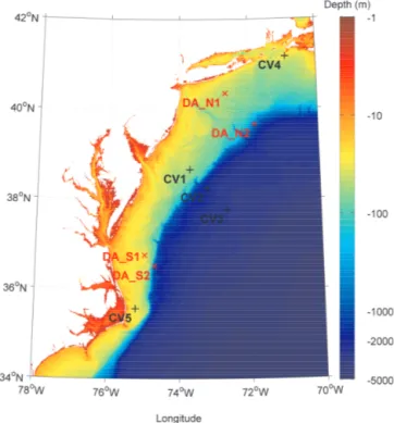
The five ecosystem models were implemented in the frame-work described above at nine locations (Fig. 1) in the Mid-Atlantic Bight (MAB). Four of these sites were designated as “data assimilation” (DA) sites, since these are the loca-tions at which data were assimilated. Two sites were selected on the inner shelf, and two were chosen just seaward of the shelf break, with two of the sites being located in the north-ern portion of the MAB and two in the southnorth-ern portion. The remaining five sites were designated as “cross-validation” (CV) sites, since these were sites where the optimal param-eters derived from assimilating data at the DA sites were in-dependently tested. These sites were spread throughout the northern, central and southern MAB, with some sites located in shallow shelf waters, and other sites located off the shelf in deep (>2000 m) waters. Three experiments were conducted at these nine sites, and are described in more detail below.
– Experiment 1: each model was implemented in a for-ward model run at all nine sites, and a priori cost func-tions (both Size_cost and Total_cost) from these pre-assimilation simulations were computed.
– Experiment 2: POC data and size-fractionated chloro-phyll data from the four DA sites were assimilated into each of the five models to determine a single best-fit set of parameter values for these four sites. The result-ing cost functions (both Size_cost and Total_cost) were computed both at the four DA sites, as well as at the five CV sites.
– Experiment 3: to determine the robustness of the opti-mal parameters determined in experiment 2 and the sen-sitivity of these parameter values to uncertainties asso-ciated with the satellite-derived products, normally dis-tributed random noise with a maximum amplitude of 20 % was added to the size-fractionated chlorophyll and POC data from the four DA sites prior to assimilation.
Figure 1. Locations of the nine study sites in the Mid-Atlantic Bight. The red crosses represent the four data assimilation (DA) sites, and the black pluses the five cross-validation (CV) sites.
The resulting optimal parameter values were compared to those determined in experiment 2. Cost functions for the four DA and five CV sites were computed as mis-fits between the simulations using these new optimal parameter values and the noisy data.
3 Results
3.1 Experiment 1: a priori simulation
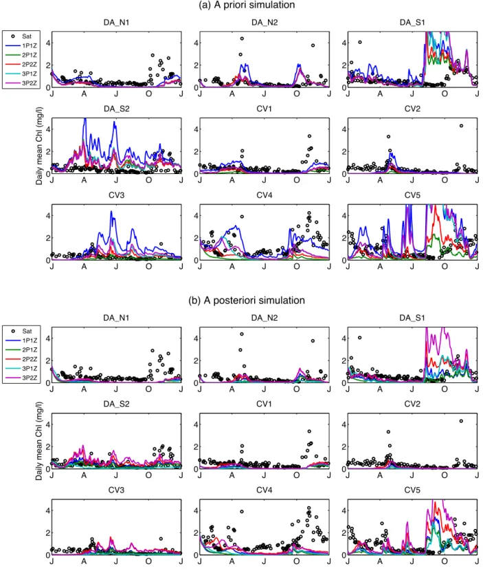
All five a priori surface chlorophyll simulations from the five different models were comparable at most of the nine sites, in particular at the northern sites such as N1, N2, CV1 and CV2 (Fig. 2a). More variability between models was found at the southern sites and offshore sites. For example, the model es-timates of the peak chlorophyll during the fall bloom ranged from 2 mg Chl m−3(the 2P1Z model) to>5 mg Chl m−3(the 3P2Z model) at the CV5 site. The 1P1Z model stood out from the other four models in that it tended to produce slightly higher chlorophyll concentrations at most of the sites, while it still gave similar estimates on the bloom timing to the other models (Fig. 2a).
42
J A J O J
0 2 4
DA_N1
J A J O J
0 2 4
DA_N2
J A J O J
0 2 4
DA_S1
Sat 1P1Z 2P1Z 2P2Z 3P1Z 3P2Z
J A J O J
0 2 4
Daily mean Chl (mg/l)
DA_S2
J A J O J
0 2 4
CV1
J A J O J
0 2 4
CV2
J A J O J
0 2 4
CV3
J A J O J
0 2 4
CV4
(a) A priori simulation
J A J O J
0 2 4
CV5
43
J A J O J
0 2 4
DA_N1
J A J O J
0 2 4
DA_N2
J A J O J
0 2 4
DA_S1
Sat 1P1Z 2P1Z 2P2Z 3P1Z 3P2Z
J A J O J
0 2 4
Daily mean Chl (mg/l)
DA_S2
J A J O J
0 2 4
CV1
J A J O J
0 2 4
CV2
J A J O J
0 2 4
CV3
J A J O J
0 2 4
CV4
(b) A posteriori simulation
J A J O J
0 2 4
CV5
Figure 2.Time series of total surface chlorophyll from the satellite-derived data (open black circles) and the(a)a priori and(b)a posteriori simulations (lines) at the nine study sites for the five ecosystem models.
the 3P models, model estimates of ChlM were also consid-erably lower than ChlS throughout the year at all nine sites. For all 2P and 3P models, ChlS was the dominant chlorophyll component throughout most of the year.
Although all models failed to capture some key features of the surface chlorophyll distributions (Fig. 2a) such as bloom timing (e.g., at site DA_S1) and magnitude (e.g., at site DA_N2), in general, all five models fit the satellite-derived surface total chlorophyll and POC distributions similarly
well. The general consistency in the five model simulations resulted in the a priori cost functions of the five models being relatively comparable. At both the DA sites (Table 3) and the CV sites (Table 4) the a priori Total_cost was highest for the simplest 1P1Z model, primarily as a result of an overestimate of surface chlorophyll at the DA_S2 site and the offshore CV3 site (Fig. 2a). The 3P models performed only slightly better, as they significantly overestimated chlorophyll at the CV5 site near Cape Hatteras (Fig. 2a). In terms of reproduc-ing the size fractionation data (Size_cost), the 2P models per-formed best, regardless of whether or not they included a sec-ond zooplankton component (Tables 3, 4). In terms of the 3P models, the model with the second zooplankton component produced slightly lower a priori Size_costs.
3.2 Experiment 2: assimilation of satellite-derived data 3.2.1 Experiment 2 results at data assimilation (DA)
sites
The assimilation of size-differentiated chlorophyll and POC data at the four DA sites resulted in significant reductions in Size_cost (Table 3), indicating successful optimizations for all five models. Improvements in model–data misfit were most substantial at the two southern stations (DA_S1 and DA_S2) (Fig. 2b). As expected from the previous results of Xiao and Friedrichs (2014), this reduction in Size_cost was accomplished primarily through improvements in chloro-phyll model–data fit (Fig. 3a and b). The assimilation par-ticularly improved model–data misfit for the smallest size class of chlorophyll for all five models. The 2Z models also produced improved model–data fits for other size classes of chlorophyll, but this was not the case for the 1Z models.
Although Size_cost cannot be used to quantitatively com-pare the skill of all five models (see Sect. 2.3), it is still a useful metric for comparison of models with the same numbers of phytoplankton variables. Somewhat surprisingly, Size_cost was lower (and percent reduction in cost much greater) for models with only one zooplankton size class than for those with two zooplankton size classes. This effect was stronger for the more complex 3P models than for the 2P models (Table 3).
In order to compare models with different phytoplankton structures, Total_cost was computed to represent the model– data misfits of total chlorophyll and POC (Table 3, Fig. 3c). After assimilation, Total_cost decreased for all models (mean decrease of∼30 %), which was only slightly smaller than the analogous decrease of Size_cost (mean decrease of∼40 %). The lowest a posteriori costs were found with the simplest 1P and 2P models, and the highest cost was obtained using the most complex 3P2Z model. The decrease in cost function was attained almost entirely through the decrease in chloro-phyll cost (mean decrease of∼55 %).
Optimal parameters generated by the five models were all well constrained (Fig. 4a). Out of the 29 optimized
parame-2P1Z 2P2Z
0 10 20 30
Size_cost
(a)
ChlS ChlL POC
3P1Z 3P2Z
0 10 20 30
(b)
ChlS ChlM ChlL POC
1P1Z 2P1Z 2P2Z 3P1Z 3P2Z
0 10 20 30
Total_cost
(c)
Total Chl POC
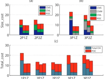
Figure 3.Cost functions at the four DA sites:(a)Size_cost for the 2P models,(b)Size_cost for the 3P models and(c)Total_cost for all five models. The three bars (from left to right) for each model represent the costs obtained for experiment 1 (a priori cost), exper-iment 2 (a posteriori cost) and experexper-iment 3 (a posteriori case with noise), respectively. Colors represent the various components (total chlorophyll, size-fractionated chlorophyll and POC) of these costs.
ters for the 5 models, only 7 of these represented a change of greater than 50 %. Both 2Z models showed only minor changes in parameter values, whereas the three 1Z models all had at least one parameter that changed by more than 50 %. The large changes in parameter values for these 1Z models are consistent with the largest reductions in costs for these models, as discussed above. However, the 2P2Z model fit the total chlorophyll data (Total_cost = 11.2) nearly as well as the 2P1Z model (Total_cost = 10.8), despite much smaller changes to the a priori parameter values. Specifically, the su-perior fit of the 2P1Z model was obtained only when the maximum Chl : C ratio for micro-phytoplankton was unre-alistically reduced by an order of magnitude.
Among the three types of optimized parameters, the max-imum phytoplankton growth rate was adjusted the least by the optimization, suggesting that these parameters were ini-tialized near their optimal values. Greater variations in op-timal values were found with the other parameters, without any clear patterns forming as a function of model structure.
Table 3.Cost functions (Size_cost and Total_cost) computed at the four DA sites in experiment 2, using initial parameter values (i.e., a priori cost) and optimal parameter values obtained from the assimilation of satellite-derived size-fractionated chlorophyll and POC data at the four DA sites (i.e., a posteriori cost).
Model
Size_cost Total_cost
a priori a posteriori % a priori a posteriori % cost cost change cost cost change
1P1Z 22.0 11.6 −47 % 22.0 11.6 −47 % 2P1Z 15.1 9.4 −37 % 13.3 10.8 −19 % 2P2Z 14.9 10.9 −26 % 12.8 11.2 −12 % 3P1Z 22.8 8.5 −63 % 20.0 12.4 −38 % 3P2Z 19.5 13.9 −29 % 20.1 15.8 −21 %
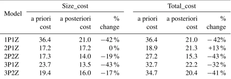
Table 4.Cost functions (Size_cost and Total_cost) computed at the five independent CV sites in experiment 2, using initial parameter values (i.e., a priori cost) and optimal parameter values obtained from the assimilation of satellite-derived size-fractionated chlorophyll and POC data at the four DA sites (i.e., a posteriori cost).
Model
Size_cost Total_cost
a priori a posteriori % a priori a posteriori % cost cost change cost cost change
1P1Z 36.4 21.0 −42 % 36.4 21.0 −42% 2P1Z 17.2 17.2 0 % 18.9 21.3 +13 % 2P2Z 17.3 14.0 −19 % 27.2 15.3 −43 % 3P1Z 23.7 13.5 −43 % 32.7 22.2 −32 % 3P2Z 19.4 16.0 −17 % 34.7 20.4 −41 %
all models except the 2P1Z model (Table 4, Fig. 5a, b). The greatest reductions in Size_cost at the CV sites occurred for the 3P1Z and 1P1Z models (∼40 %), which was equivalent to the reductions in Size_cost generated by these models at the DA sites. Significant, but smaller, reductions also oc-curred for the 2P2Z and 3P2Z models (∼20 %, Table 4). All five models showed an increase in the POC cost; however the improvement in model–data fit for size-fractionated chloro-phyll, particularly for the smallest chlorophyll size class, more than compensated for the deterioration in POC model– data misfit in all cases except for the 2P1Z model (Fig. 5a and b).
Applying the optimal parameters from the DA sites to sim-ulations at the CV sites also generated significant improve-ments in the total chlorophyll cost for each of the five mod-els (Fig. 5c). This decrease in total chlorophyll cost was again substantially larger than the increase in POC cost for all mod-els except the 2P1Z model, and thus the overall Total_cost also decreased for four of the five models (Table 4). The lack of improvement for the 2P1Z model is at least partially due to the fact that using the a priori parameter values with the 2P1Z model generated an a priori simulation that fit the data at the five CV sites very well (Fig. 5c). In fact the a priori Total_cost for the 2P1Z model was lower than the a poste-riori Total_cost of the 1P and 3P models (Table 4, Fig. 5c). Overall, the intermediately complex 2P2Z model produced
the lowest Total_cost when using the parameters optimized for the DA sites at the CV sites.
3.3 Experiment 3: assimilation of perturbed data 3.3.1 Experiment 3 results at data assimilation (DA)
sites
The a priori costs for experiment 3 were computed as the dif-ference between the a priori simulations and the noisy data, and were only very slightly different (<1 %) from the a pri-ori costs for experiment 2, which were computed as the dif-ference between the a priori simulations and the actual data. When the noisy data were assimilated into the models at the four DA sites in experiment 3, the optimization process generated very similar parameters to those generated in ex-periment 2 for the 1P, 2P and 3P1Z models (Fig. 4). Thus the addition of random noise did not significantly affect the op-timization process for these simpler models, and as a result the a posteriori Size_costs resulting from the assimilation of the noisy data were almost identical to those generated by assimilating the actual data (Fig. 3).
In contrast, the optimal parameters generated in exper-iment 3 for the most complex 3P2Z model were signif-icantly different from those in experiment 2 (Fig. 4b). For example, the optimal value for the maximum Chl : C ratio for pico-phytoplankton in the 3P2Z model was
1P1Z 2P1Z 2P2Z 3P1Z 3P2Z 0
1 2 3 4
Normalized parameters
(a) Expt. 2
Max Chl:C Max P growth rate Z basal metabolism
1P1Z 2P1Z 2P2Z 3P1Z 3P2Z 0
1 2 3 4
Normalized parameters
(b) Expt. 3
Figure 4.Optimized parameter values normalized to a priori values obtained(a)by assimilating POC and size-fractionated data at the four DA sites (experiment 2), and(b)by assimilating satellite data to which 20 % random noise has been added (experiment 3).
2P1Z 2P2Z 0
10 20 30 40
Size_cost
(a)
ChlS ChlL POC
3P1Z 3P2Z 0
10 20 30 40
(b)
ChlS ChlM ChlL POC
1P1Z 2P1Z 2P2Z 3P1Z 3P2Z 0
10 20 30 40
Total_cost
(c)
Total Chl POC
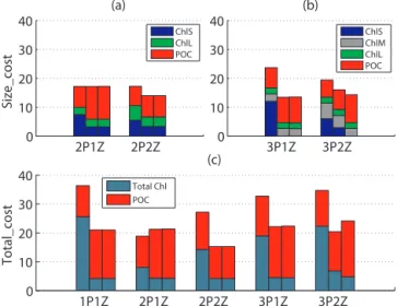
Figure 5.Cost functions at the five CV sites:(a)Size_cost for the 2P models,(b)Size_cost for the 3P models and(c)Total_cost for all five models. The three bars (from left to right) for each model represent the costs obtained for experiment 1 (a priori cost), exper-iment 2 (a posteriori cost) and experexper-iment 3 (a posteriori case with noise), respectively. Colors represent the various components (total chlorophyll, size-fractionated chlorophyll and POC) of these costs.
6.1×10⁻¹³mg Chl mg C−1 compared to a value of 0.023 generated when assimilating the actual satellite-derived data. As a result, this new set of optimal parameter values (Fig. 4b) resulted in a significantly different Size_cost (∼35 % de-crease). This decrease in the 3P2Z Size_cost was caused by
a substantial reduction in the cost components of ChlS and ChlM, whereas the contribution of ChlL and POC remained nearly unchanged (Fig. 3b).
3.3.2 Experiment 3 results at cross-validation (CV) sites The costs at the CV sites for the 1P, 2P and 3P1Z models were nearly identical for experiments 2 and 3 (Fig. 5). This was true despite some significant changes in the optimized parameter values for the 3P1Z model (Fig. 4): for example, the zooplankton basal metabolism rate was twice as high in experiment 3 compared to experiment 2. As was the case at the DA sites, the 3P2Z a posteriori costs were much more sensitive to the noise added to the data prior to assimilation. Although the a posteriori 3P2Z Size_cost decreased for the ChlS and ChlM components, the a posteriori Total_cost in-creased due to a significant deterioration in the model–data fit for POC.
In summary, the addition of noise to the assimilated data had almost no effect on the cost functions for the simpler models, but significantly affected the costs of the most com-plex (3P2Z) model. Although the 3P2Z model showed im-provement in model–data misfit at the DA sites with the ad-dition of noise prior to assimilation, it was attained at the expense of unreasonable optimized parameter values and an increase in the Total_cost at the independent cross-validation sites.
4 Discussion and conclusions
In this study, five lower-trophic-level ecosystem models with varying food web complexities were rigorously compared in order to determine how the number of phytoplankton and zooplankton compartments affects the ability of a lower-trophic-level model to reproduce observed patterns in surface chlorophyll and particulate organic carbon. All five models were embedded in a 1-D assimilative model framework with identical physics and biogeochemical formulations, and thus the differences in the model simulations were only a result of variations in the complexity of the planktonic food web structure.
This is most likely due to issues related to the physical fields obtained from the 3-D simulation used to force these models. Interestingly, the a posteriori parameters optimized for these five models were very different for the different mod-els. In particular, the models with a single zooplankton size class were only able to reproduce the assimilated data us-ing extremely low zooplankton basal metabolism rates, or extremely low maximum Chl : C ratios, whereas the mod-els with two zooplankton size classes were able to reproduce the POC and chlorophyll observations using realistic rates and ratios. Ultimately, the parameters optimized for the two-phytoplankton, two-zooplankton (2P2Z) model were most similar to our best-guess a priori initial parameter values.
The improvements in model skill for all five models were not limited to the four specific sites where the data were as-similated. Rather, a cross-validation analysis demonstrated that the parameters optimized for these four sites within the MAB improved the simulations at a number of other sites throughout the region, giving us confidence in the portabil-ity of these optimized parameter values and optimism for the potential success of using these parameters in a three-dimensional simulation of the US eastern continental shelf (McDonald et al., 2012). Although almost all models showed some degree of improvement at these other MAB sites, once again the model characterized by intermediate complexity (i.e., 2P2Z) performed best. The other models were able to fit the data at the assimilation sites equally as well as the 2P2Z model; however, they typically did so by using unreal-istic parameter values which were not portable to other areas of the MAB.
Intriguing results were also obtained when random noise was added to the satellite-derived data prior to assimilation. The addition of the noise perturbation had almost no effect on the values of the optimized parameters for the simplest four models, suggesting that the optimization process was robust for these models, even when significant noise was present in the assimilated data. However, when these per-turbed data were assimilated into the most complex model (the 3P2Z model), substantially different optimal parameter values were obtained. For certain parameters (e.g., the maxi-mum Chl : C ratio for pico-phytoplankton), the difference be-tween the optimized parameter values obtained by assimilat-ing the actual data versus those obtained by assimilatassimilat-ing the noisy data was more than 10 orders of magnitude. Although the new parameter values obtained by assimilating the noisy data improved the model–data fit at the specific sites where the data were assimilated, the unrealistic parameter values deteriorated the model performance at other sites within the MAB. In essence, unlike the simpler models, the most com-plex model had enough flexibility that it was actually able to fit the additional noise artificially added to the data. Al-though this “over-tuning” actually improved the model–data fit at the sites where the noisy data were assimilated, this is a dangerous outcome, as the model–data fit was degraded at
other locations within the MAB where data were not avail-able for assimilation.
This over-tuning issue for complex models has been al-luded to in previous studies. For example, Friedrichs et al. (2006) assimilated data during three seasons of the year, and cross-validated the resulting optimal parameters against the data in the remaining season. Their cross-validation ex-periments showed that complex models with too many un-constrained parameters might be able to fit the assimilated data extremely well (the more free parameters, the better the fit to the assimilated data), yet these complex models would have poor predictive ability (the more free parameters, the worse the fit to independent, unassimilated data).
Another difficulty with complex models is that they are usually governed by such a large number of parameters (the number of parameters that must be specified in a given ecosystem model generally increases by as much as the square of the number of state variables; Denman, 2003), that it is very difficult to identify the best-fit set of parameters. When hand-tuning such models, there are simply too many different parameters to adequately test all parameter combi-nations. When applying an automated parameter optimiza-tion method such as the variaoptimiza-tional adjoint method to com-plex models with multiple unconstrained parameters, the cost function has a tendency to get stuck in suboptimal “local minima”, and as a result the absolute global cost function minimum and the true “best-fit” set of parameters can poten-tially never be identified. In fact, this is exactly what occurred in the present study for the most complex 3P2Z model. The a posteriori cost function was highest for this model, despite the presumably increased flexibility that this model had to fit the data, because the cost function became stuck in a lo-cal minimum. However, when artificial noise was added to the data prior to assimilation, an alternate local cost function minimum was identified, which, somewhat surprisingly, was smaller than the one identified when the true data were assim-ilated. The problem of complex models becoming stuck in local cost function minima has also been discussed by other authors. For example, Ward et al. (2010) demonstrated that when too many unconstrained parameters were optimized, the cost function often became trapped in a local minimum; however, reducing the number of optimized parameters par-tially eliminated this problem.
Our conclusion that an intermediate complexity model is the most ideally suited for regional ecosystem studies is consistent with results from earlier studies using other types of models without the formal parameter optimiza-tion techniques employed here. For example, an early study by Costanza and Sklar (1985) rated 87 models in wetland and shallow water bodies in terms of 3 indices: articula-tion (the complexity of the model), accuracy (goodness of fit of the model to the data) and effectiveness (trade-off be-tween complexity and accuracy). They concluded that al-though the accuracy seemed to increase with articulation, the maximum effectiveness was found at an intermediate level of
complexity. Fulton et al. (2003) found a similar humped re-lationship between model complexity and performance when examining end-to-end (nutrient to fisheries) models, demon-strating that the best performance was produced by the model with intermediate complexity. Another model comparison study was conducted by Raick et al. (2006), in which three simplified pelagic ecosystem models with 16, 9 and 4 state variables, respectively, were assessed according to their abil-ity to reproduce simulations from performance of a complex model with 19 state variables. The study found that although the simplest model (4 state variables) was able to capture the key features demonstrated by the complex model, the model with intermediate complexity (9 state variables) most closely reproduced the output from the full 19 state-variable model.
Appendix A: Model equations
The equations for each of the five models are included be-low for reference. State variables are defined as folbe-lows: P, total phytoplankton; Z, total zooplankton; SD, small de-tritus; LD, large dede-tritus; NO3, nitrate; NH4, ammonium; Chl, chlorophyll; SP, small phytoplankton; MP, medium phy-toplankton; LP, large phyphy-toplankton; SZ, small zooplank-ton; LZ, large zooplankzooplank-ton; SChl, small chlorophyll; MChl, medium chlorophyll; and LChl, large chlorophyll. Parameter values, except for those specifically noted in text and Table 1, are provided in Fennel et al. (2006, 2008). As an example, generic functional formulations are listed below for SP and SZ, but analogous formulations hold for the medium (MP, MZ), large (LP, LZ) and single (P, Z) size classes.
Functional formulations (example for SP, SZ)
gSP_SZ=gmax_SP_SZ SP2 kP+SP2 ρSChl=
θmax_SPµSP·SP αI·SChl fSP(I )=
αI
q
µ2max_SP+α2I2
LNO3_SP=
NO3
kNO3_SP+NO3 1+ NH4 kNH4
−1
LNH4=
NH4 kNH4+NH4
µSP=µmax_SPfSP(I )(LNO3_SP+LNH4)
µSP_NO3=µmax_SPfSP(I )LNO3_SP
µSP_NH4=µmax_SPfSP(I )LNH4
1P1Z (includes P, Z) ∂P
∂t =µPP−gP_ZZ−mPP−τ (SD+P)P−wP ∂P dz ∂Z
∂t =gP_ZβZ−lBM_ZZ−lE P2
kP+P2βZ−mZZ 2
∂SD
∂t =gP_Z(1−β)Z+mZZ
2+mPP−τ (SD+P)SD
−rSDSD−wSD ∂SD
∂z ∂LD
∂t =τ (SD+P) 2−r
LDLD−wLD ∂LD
∂z ∂NO3
∂t = −µP_NO3P+nNH4 ∂NH4
∂t = −µP_NH4P−nNH4+lBM_ZZ+lE P2 kP+P2βZ +rSDSD+rLDLD
∂Chl
∂t =ρChlµPChl−gP_ZZ Chl
P −mPChl−τ (SD+P)Chl
2P1Z (includes SP, LP, Z)
∂SP
∂t =µSPSP−gSP_ZZ−mPSP−τ (SD+P)SP−wSP ∂SP
dz ∂LP
∂t =µLPLP−gLP_ZZ−mPLP−τ (SD+P)LP−wLP ∂LP
dz ∂Z
∂t =(gSP_Z+gLP_Z)βZ−lBM_ZZ−lE P2 kP+P2
βZ−mZZ2 ∂SD
∂t =(gSP_Z+gLP_Z)(1−β)Z+mZZ 2+m
PP −τ (SD+P)SD−rSDSD−wSD∂SD
∂z ∂LD
∂t =τ (SD+P) 2−r
LDLD−wLD ∂LD
∂z ∂NO3
∂t = −µSP_NO3SP−µLP_NO3LP+nNH4 ∂NH4
∂t = −µSP_NH4SP−µLP_NH4LP−nNH4+lBM_ZZ +lE
P2 kP+P2
βZ+rSDSD+rLDLD ∂SChl
∂t =ρSChlµSPSChl−gSP_ZZ SChl
SP −mPSChl −τ (SD+P)SChl
∂LChl
∂t =ρLChlµLPLChl−gLP_ZZ LChl
LP −mPLChl −τ (SD+P)LChl
2P2Z (includes SP, LP, SZ, LZ)
∂SP
∂t =µSPSP−gSP_SZSZ−gSP_LZLZ−mPSP −τ (SD+P)SP−wSP
∂SP dz ∂LP
∂t =µLPLP−gLP_SZSZ−gLP_LZLZ−mPLP −τ (SD+P)LP−wLP
∂LP dz ∂SZ
∂t =(gSP_SZ+gLP_SZ)βSZ−lBM_SZSZ−lE P2 kP+P2
βSZ
−mZSZ2 ∂LZ
∂t =(gSP_LZ+gLP_LZ)βLZ−lBM_LZLZ−lE P2 kP+P2βLZ −mZLZ2
∂SD
∂t =(gSP_SZ+gLP_SZ)(1−β)SZ
+(gSP_LZ+gLP_LZ)(1−β)LZ+mZSZ2+mZLZ2 +mPP−τ (SD+P)SD−rSDSD−wSD
∂SD ∂z
∂LD
∂t =τ (SD+P) 2−rLD
LD−wLD∂LD ∂z ∂NO3
∂t = −µSP_NO3P−µLP_NO3P+nNH4 ∂NH4
∂t = −µSP_NH4P−µLP_NH4P−nNH4+lBM_SZSZ +lBM_LZLZ+lE
P2
kP+P2βZ+rSDSD+rLDLD ∂SChl
∂t =ρSChlµSPSChl−gSP_SZSZ SChl
SP −gSP_LZLZ SChl
SP −mPSChl−τ (SD+P)SChl
∂LChl
∂t =ρLChlµLPLChl−gLP_SZSZ LChl
LP −gLP_LZLZ LChl
LP −mPLChl−τ (SD+P)LChl
3P1Z (includes SP, MP, LP, Z) ∂SP
∂t =µSPSP−gSP_ZZ−mPSP−τ (SD+P)SP −wSP
∂SP dz ∂MP
∂t =µMPMP−gMP_ZZ−mPMP−τ (SD+P)MP −wMP∂MP
dz ∂LP
∂t =µLPLP−gLP_ZZ−mPLP−τ (SD+P)LP −wLP
∂LP dz ∂Z
∂t =(gSP_Z+gMP_Z+gLP_Z)βZ−lBM_ZZ −lE P
2
kP+P2βZ−mZZ 2
∂SD
∂t =(gSP_Z+gMP_Z+gLP_Z)(1−β)Z+mZZ 2+m
PP −τ (SD+P)SD−rSDSD
−wSD∂SD ∂z ∂LD
∂t =τ (SD+P) 2−r
LDLD−wLD ∂LD
∂z ∂NO3
∂t = −µSP_NO3P−µMP_NO3P−µLP_NO3P+nNH4 ∂NH4
∂t = −µSP_NH4P−µMP_NH4P−µLP_NH4P−nNH4 +lBM_ZZ+lE
P2 kP+P2
βZ+rSDSD+rLDLD ∂SChl
∂t =ρSChlµSPSChl−gSP_ZZ SChl
SP −mPSChl −τ (SD+P)SChl
∂MChl
∂t =ρMChlµMPMChl −gMP_ZZ MChl
MP −mPMChl −τ (SD+P)MChl
∂LChl
∂t =ρLChlµLPLChl−gLP_ZZ LChl
LP −mPLChl −τ (SD+P)LChl
3P2Z (includes SP, MP, LP, SZ, LZ)
∂SP
∂t =µSPSP−gSP_SZSZ−gSP_LZLZ−mPSP −τ (SD+P)SP−wSP
∂SP dz ∂MP
∂t =µMPMP−gMP_SZSZ−gMP_LZLZ−mPMP −τ (SD+P)MP−wMP∂MP
dz ∂LP
∂t =µLPLP−gLP_SZSZ−gLP_LZLZ−mPLP −τ (SD+P)LP−wLP
∂LP dz ∂SZ
∂t =(gSP_SZ+gMP_SZ+gLP_SZ)βSZ−lBM_SZSZ −lE
P2
kP+P2βSZ−mZSZ 2
∂LZ
∂t =(gSP_LZ+gMP_LZ+gLP_LZ)βLZ−lBM_LZLZ −lE
P2
kP+P2βLZ−mZLZ 2
∂SD
∂t =(gSP_SZ+gMP_SZ+gLP_SZ)(1−β)SZ +(gSP_LZ+gMP_LZ+gLP_LZ)(1−β)LZ +mZSZ2+mZLZ2+mPP−τ (SD+P)SD −rSDSD−wSD
∂SD ∂z ∂LD
∂t =τ (SD+P) 2−r
LDLD−wLD ∂LD
∂z ∂NO3
∂t = −µSP_NO3P−µMP_NO3P−µLP_NO3P+nNH4 ∂NH4
∂t = −µSP_NH4P−µMP_NH4P−µLP_NH4P−nNH4 +lBM_SZSZ+lBM_LZLZ+lE P
2
kP+P2
βZ+rSDSD +rLDLD
∂SChl
∂t =ρSChlµSPSChl−gSP_SZSZ SChl
SP −gSP_LZLZ SChl
∂MChl
∂t =ρMChlµMPMChl−gMP_SZSZ SChl
MP −gMP_LZLZ
MChl
MP −mPMChl −τ (SD+P)MChl ∂LChl
∂t =ρLChlµLPLChl−gLP_SZSZ LChl
LP −gLP_LZLZ LChl
LP −mPLChl−τ (SD+P)LChl
Acknowledgements. This work was supported by the NASA Earth and Space Science Fellowship Program (grant NNX10AN50H) and the NASA Interdisciplinary Science Program (NNX11AD47G). The authors are grateful to the NASA US Eastern Continental Shelf Carbon Cycling (USECoS) team for their useful comments, especially Kimberly Hyde, Antonio Mannino and Xiaoju Pan for providing the satellite-derived size-fractionated chlorophyll data. The authors would like to thank the SeaWiFS Project (code 970.2) and the Distributed Active Archive Center (code 610.2) at the Goddard Space Flight Center, Greenbelt, MD 20771, for the production and distribution of these data, respectively. This is VIMS contribution no. 3342.
Edited by: K. Fennel
References
Anderson, T. R.: Plankton functional type modelling: running before we can walk?, J. Plankton Res., 27, 1073–1081, doi:10.1093/plankt/fbi076, 2005.
Baird, M. E. and Suthers, I. M.: Increasing model structural com-plexity inhibits the growth of initial condition errors, Ecol. Com-plex., 7, 478–486, doi:10.1016/j.ecocom.2009.12.001, 2010. Bagniewski, W., Fennel, K., Perry, M. J., and D’Asaro, E. A.:
Op-timizing models of the North Atlantic spring bloom using phys-ical, chemical and bio-optical observations from a Lagrangian float, Biogeosciences, 8, 1291–1307, doi:10.5194/bg-8-1291-2011, 2011.
Costanza, R. and Sklar, F. H.: Articulation, accuracy and effec-tiveness of mathematical models: A review of freshwater wet-land applications, Ecol. Model., 27, 45–68, doi:10.1016/0304-3800(85)90024-9, 1985.
Denman, K. L.: Modelling planktonic ecosystems: Parameterizing complexity, Progr. Oceanogr., 57, 429–452, 2003.
Fan, W. and Lv, X.: Data assimilation in a simple marine ecosys-tem model based on spatial biological parameterizations, Ecol. Model., 220, 1997–2008, doi:10.1016/j.ecolmodel.2009.04.050, 2009.
Fennel, K., Wilkin, J., Levin, J., Moisan, J., O’Reilly, J., and Haid-vogel, D.: Nitrogen cycling in the Middle Atlantic Bight: Results from a three-dimensional model and implications for the North Atlantic nitrogen budget, Global Biogeochem. Cy., 20, GB3007, doi:10.1029/2005gb002456, 2006.
Flynn, K. J.: Castles built on sand: dysfunctionality in plankton models and the inadequacy of dialogue between biologists and modellers, J. Plankton Res., 27, 1205–1210, 2005.
Follows, M. J., Dutkiewicz, S., Grant, S., and Chisholm, S. W.: Emergent biogeography of microbial communities in a model ocean, Science, 315, 1843–1846, doi:10.1126/science.1138544, 2007.
Friedrichs, M. A. M.: The assimilation of SeaWiFS and JGOFS Eq-Pac data into a marine ecosystem model of the central equatorial Pacific, Deep-Sea Res. Pt. II, 49, 289–319, 2002.
Friedrichs, M. A. M., Hood, R. R., and Wiggert, J. D.: Ecosystem model complexity versus physical forcing: Quantification of their relative impact with assimilated Arabian Sea data, Deep-Sea Res. Pt. II, 53, 576–600, doi:10.1016/j.dsr2.2006.01.026, 2006. Friedrichs, M. A. M., Dusenberry, J., Anderson, L., Armstrong,
R., Chai, F., Christian, J.,Doney, S. C., Dunne, J., Fujii, M.,
Hood, R., McGillicuddy, D., Moore, K., Schartau, M., Sp-tiz, Y. H., and Wiggert, J.: Assessment of skill and portabil-ity in regional marine biogeochemical models: role of mul-tiple phytoplankton groups, J. Geophys. Res., 112, C08001, doi:10.1029/2006JC003852, 2007.
Friedrichs, M. A. M., Carr, M.-E., Barber, R., Scardi, M., Antoine, D., Armstrong, R. A., Asanuma, I., Behrenfeld, M. J., Buiten-huis, E. T., Chai, F., Christian, J. R., Ciotti, A. M., Doney, S., C., Dowell, M., Dunne, J., Gentili, B., Gregg, W., Hoepffner, N., Ishizaka, J., Kameda, T., Lima, I., Marra, J., Mélin, F., Moore, J. K., Morel, A., O’Malley, R. T., O’Reilly, J., Saba, V. S., Schmeltz, M., Smyth, T. J., Tjiputra, J., Waters, K., Westberry, T. K., and Winguth, A.: Assessing the uncertainties of model estimates of primary productivity in the tropical Pacific Ocean, J. Mar. Syst., 76, 113–133, doi:10.1016/j.jmarsys.2008.05.010, 2009.
Fulton, E. A., Smith, A. D. M., and Johnson, C. R.: Effect of com-plexity on marine ecosystem models, Mar. Ecol.-Prog. Ser., 253, 1–16, doi:10.3354/meps253001, 2003.
Garcia-Gorriz, E., Hoepffner, N., and Ouberdous, M.: Assimila-tion of SeaWiFS data in a coupled physical-biological model of the Adriatic Sea, J. Mar. Syst., 40, 233–252, doi:10.1016/s0924-7963(03)00020-4, 2003.
Giering, R. and Kaminski, T.: Recipes for adjoint code construction, ACM T. Math. Software, 24, 437–474, doi:10.1145/293686.293695, 1998.
Gilbert, J. C. and Lemarechal, C.: Some numerical experiments with variable-storage quasi-newton algorithms, Math. Program., 45, 405–435, 1989.
Gregg, W., Friedrichs, M. A. M., Robinson, A. R., Rose, K., Schlitzer, R., and Thompson, K. R.: Skill assessment in ocean biological data assimilation, J. Mar. Syst., 76, 16–33, doi:10.1016/j.jmarsys.2008.05.006, 2009.
Hannah, C., Vezina, A., and St John, M.: The case for marine ecosystem models of intermediate complexity, Progr. Oceanogr., 84, 121–128, doi:10.1016/j.pocean.2009.09.015, 2010.
Hashioka, T., Vogt, M., Yamanaka, Y., Le Quéré, C., Buitenhuis, E. T., Aita, M. N., Alvain, S., Bopp, L., Hirata, T., Lima, I., Sail-ley, S., and Doney, S. C.: Phytoplankton competition during the spring bloom in four plankton functional type models, Biogeo-sciences, 10, 6833–6850, doi:10.5194/bg-10-6833-2013, 2013. Hemmings, J. C. P., Srokosz, M. A., Challenor, P., and Fasham,
M. J. R.: Split-domain calibration of an ecosystem model us-ing satellite ocean colour data, J. Mar. Syst., 50, 141–179, doi:10.1016/j.jmarsys.2004.02.003, 2004.
Hofmann, E., Druon, J.-N. Fennel, K., Friedrichs, M., Haidvogel, D., Lee, C., Mannino, A., McClain, C., Najjar, R., O’Reilly, J., Pollard, D., Previdi, M., Seitzinger, S., Siewert, J., Signorini, S., and Wilkin, J.: Eastern U.S. continental shelf carbon budget: in-tegrating models, data assimilation, and analysis, Oceanography, 21, 86–104, 2008.
Hofmann, E. E., Cahill, B., Fennel, K., Friedrichs, M. A. M., Hyde, K., Lee, C., Mannino, A., Najjar, R. G., O’Reilly, J. E., Wilkin, J., and Xue, J.: Modeling the dynamics of continental shelf carbon, Annu. Rev. Mar. Sci., 3, 93–122, doi:10.1146/annurev-marine-120709-142740, 2011.
cou-pled hydrodynamic-ecosystem model skill assessment, J. Mar. Syst., 76, 64–82, doi:10.1016/j.jmarsys.2008.05.014, 2009. Kishi, M. J., Kashiwai, M., Ware, D. M., Megrey, B. A., Eslinger,
D. L., Werner, F. E., Noguchi-Aita, F. M., Azumaya, T., Fujii, M., Hashimoto, S., Huang, D. J., Iizumi, H., Ishida, Y., Kang, S., Kantakov, G. A., Kim, H. C., Komatsu, K., Navrotsky, V. V., Smith, S. L., Tadokoro, K., Tsuda, A., Yamamura, O.,Yamanaka, Y., Yokouchi, K., Yoshie, N., Zhang, J., Zuenko, Y. I., and Zvalinsky, V. I.: NEMURO – a lower trophic level model for the North Pacific marine ecosystem, Ecol. Model., 202, 12–25, doi:10.1016/j.ecolmodel.2006.08.021, 2007.
Lawson, L. M., Spitz, Y. H., Hofmann, E. E., and Long, R. B.: A data assimilation technique applied to a predator-prey model, B. Math. Biol., 57, 593–617, doi:10.1016/S0092-8240(05)80759-1, 1995.
Lawson, L. M., Hofmann, E. E., and Spitz, Y. H.: Time series sampling and data assimilation in a simple marine ecosystem model, Deep-Sea Res. Pt. II, 43, 625–651, doi:10.1016/0967-0645(95)00096-8, 1996.
Lehmann, M. K., Fennel, K., and He, R.: Statistical validation of a 3-D bio-physical model of the western North Atlantic, Biogeo-sciences, 6, 1961–1974, doi:10.5194/bg-6-1961-2009, 2009. McDonald, C. P., Bennington, V., Urban, N. R., and
McKin-ley, G. A.: 1-D test-bed calibration of a 3-D Lake Su-perior biogeochemical model, Ecol. Model., 225, 115–126, doi:10.1016/j.ecolmodel.2011.11.021, 2012.
Pan, X., Mannino, A., Russ, M. E., Hooker, S. B., and Harding Jr., L. W.: Remote sensing of phytoplankton pigment distribution in the United States northeast coast, Remote Sens. Environ., 114, 2403–2416, doi:10.1016/j.rse.2010.05.015, 2010.
Paudel, R. and Jawitz, J. W.: Does increased model com-plexity improve description of phosphorus dynamics in a large treatment wetland?, Ecol. Eng., 42, 283–294, doi:10.1016/j.ecoleng.2012.02.014, 2012.
Raick, C., Soetaert, K., and Gregoire, M.: Model complexity and performance: How far can we simplify?, Progr. Oceanogr., 70, 27–57, doi:10.1016/j.pocean.2006.03.001, 2006.
Rykiel, E. J.: Testing ecological models: The meaning of validation, Ecol. Model., 90, 229–244, doi:10.1016/0304-3800(95)00152-2, 1996.
Salihoglu, B. and Hofmann, E. E.: Simulations of phytoplankton species and carbon production in the equatorial Pacific Ocean 1. Model configuration and ecosystem dynamics, J. Mar. Res., 65, 219–273, 2007.
Stow, C. A., Jolliff, J., McGillicuddy Jr., D. J., Doney, S. C., Allen, J. I., Friedrichs, M. A. M., Rose, K. A., and Wallhead, P.: Skill as-sessment for coupled biological/physical models of marine sys-tems, J. Mar. Syst., 76, 4–15, doi:10.1016/j.jmarsys.2008.03.011, 2009.
Stramska, M. and Stramski, D.: Variability of particulate or-ganic carbon concentration in the north polar Atlantic based on ocean color observations with Sea-viewing Wide Field-of-view Sensor (SeaWiFS), J. Geophys. Res.-Oceans, 110, C10018, doi:10.1029/2004jc002762, 2005.
Tjiputra, J. F., Polzin, D., and Winguth, A. M. E.: Assimilation of seasonal chlorophyll and nutrient data into an adjoint three-dimensional ocean carbon cycle model: Sensitivity analysis and ecosystem parameter optimization, Global Biogeochem. Cy., 21, GB1001, doi:10.1029/2006gb002745, 2007.
Ward, B. A., Friedrichs, M. A. M., Anderson, T. R., and Oschlies, A.: Parameter optimisation techniques and the problem of under-determination in marine biogeochemical models, J. Mar. Syst., 81, 34–43, doi:10.1016/j.jmarsys.2009.12.005, 2010.
Ward, B. A., Schartau, M., Oschlies, A., Martin, A. P., Fol-lows, M. J., and Anderson, T. R.: When is a biogeochemical model too complex? Objective model reduction and selection for North Atlantic time-series sites, Progr. Oceanogr., 116, 49–65, doi:10.1016/j.pocean.2013.06.002, 2013.
Xiao, Y. and Friedrichs, M. A. M.: The assimilation of satellite-derived data into a one-dimensional lower trophic level marine ecosystem model, J. Geophys. Res.-Oceans, 119, 2691–2712, doi:10.1002/2013JC009433, 2014.