Using biogeochemical data assimilation to assess the relative skill of multiple ecosystem models: effects of increasing the complexity of the planktonic food web

(1)

BGD

11, 481–520, 2014

Effects of increasing the complexity of the planktonic food web

Y. Xiao and M. A. M. Friedrichs

Title Page

Abstract Introduction

Conclusions References

Tables Figures

◭ ◮

Back Close

Full Screen / Esc

Printer-friendly Version

Interactive Discussion

Discussion

P

a

per

|

D

iscussion

P

a

per

|

Discussion

P

a

per

|

Discuss

ion

P

a

per

|

Biogeosciences Discuss., 11, 481–520, 2014 www.biogeosciences-discuss.net/11/481/2014/ doi:10.5194/bgd-11-481-2014

Open Access

Biogeosciences

Discussions

This discussion paper is/has been under review for the journal Biogeosciences (BG). Please refer to the corresponding final paper in BG if available.

Using biogeochemical data assimilation

to assess the relative skill of multiple

ecosystem models: e

_ff

ects of increasing

the complexity of the planktonic food web

Y. Xiao and M. A. M. Friedrichs

Virginia Institute of Marine Science, College of William & Mary, P.O. Box 1346, Gloucester Point, VA 23062, USA

Received: 8 December 2013 – Accepted: 20 December 2013 – Published: 8 January 2014 Correspondence to: M. A. M. Friedrichs (marjy@vims.edu)

(2)

BGD

11, 481–520, 2014

Title Page

Tables Figures

◭ ◮

Back Close

Full Screen / Esc

Discussion

P

a

per

|

D

iscussion

P

a

per

|

Discussion

P

a

per

|

Discuss

ion

P

a

per

|

Abstract

Now that regional circulation patterns can be reasonably well reproduced by ocean circulation models, significant effort is being directed toward incorporating complex food webs into these models, many of which now routinely include multiple phyto-plankton (P) and zoophyto-plankton (Z) compartments. This study quantitatively assesses

5

how the number of phytoplankton and zooplankton compartments affects the ability of a lower trophic level ecosystem model to reproduce and predict observed patterns in surface chlorophyll and particulate organic carbon. Five ecosystem model variants are implemented in a one-dimensional assimilative (variational adjoint) model testbed in the Mid-Atlantic Bight. The five models are identical except for variations in the level

10

of complexity included in the lower trophic levels, which range from a simple 1P1Z food web to a considerably more complex 3P2Z food web. The five models assimilated satellite-derived chlorophyll and particulate organic carbon concentrations at four conti-nental shelf sites, and the resulting optimal parameters were tested at five independent sites in a cross-validation experiment. Although all five models showed improvements

15

in model-data misfits after assimilation, overall the moderately complex 2P2Z model was associated with the highest model skill. Additional experiments were conducted in which 20 % random noise was added to the satellite data prior to assimilation. The 1P and 2P models successfully reproduced nearly identical optimal parameters re-gardless of whether or not noise was added to the assimilated data, suggesting that

20

random noise inherent in satellite-derived data does not pose a significant problem to the assimilation of satellite data into these models. On the contrary, the most complex model tested (3P2Z) was sensitive to the level of random noise added to the data prior to assimilation, highlighting the potential danger of overtuning inherent in such complex models.

(3)

BGD

11, 481–520, 2014

Title Page

Tables Figures

◭ ◮

Back Close

Full Screen / Esc

Discussion

P

a

per

|

D

iscussion

P

a

per

|

Discussion

P

a

per

|

Discuss

ion

P

a

per

|

1 Introduction

In spite of recent advances in marine ecosystem modeling that now allow for the incor-poration of multiple plankton functional types and/or size classes (e.g., Follows et al., 2007; Kishi et al., 2007; Salihoglu and Hofmann, 2007), it remains ambiguous whether models with additional plankton compartments necessarily perform better than

mod-5

els characterized by relatively simple structures. Although the use of a single plankton compartment may fail to resolve key processes in a given ecosystem (e.g., Ward et al., 2013), the inclusion of additional complexity in plankton structure comes with a sub-stantial cost: significant uncertainties will inevitably be associated with the additional state variables and required parameters (Anderson, 2005; Flynn, 2005). Hence these

10

trade-offs in model structure selection pose a challenging question: how does one de-termine how many phytoplankton and zooplankton compartments need to be included in a given application of a lower trophic model?

Multiple model comparison studies have helped improve our understanding of the trade-offs of increasing ecosystem model complexity, yet many of these studies have

15

not directly isolated the effects of increasing plankton complexity (e.g., Baird and Suthers, 2010; Costanza and Sklar, 1985; Fulton et al., 2003; Hannah et al., 2010; Paudel and Jawitz, 2012; Raick et al., 2006). For example, a recent community data as-similative modeling comparison exercise (Friedrichs et al., 2007) revealed that ecosys-tem models with multiple phytoplankton (P) state variables were quantitatively more

20

skillful (in terms of reproducing observations of chlorophyll, primary production, ex-port and nitrate at multiple sites) than models with single P compartments. However, the twelve models participating in the Friedrichs et al. (2007) comparison study varied in many different ways, including nutrient limitations, variable elemental compositions and zooplankton (Z) state variables, making it difficult to determine why certain

mod-25

(4)

BGD

11, 481–520, 2014

Title Page

Tables Figures

◭ ◮

Back Close

Full Screen / Esc

Discussion

P

a

per

|

D

iscussion

P

a

per

|

Discussion

P

a

per

|

Discuss

ion

P

a

per

|

it was not completely clear whether the improvement was due to the additional phy-toplankton compartment or was caused by other differences in the structures of the two models such as the variable Carbon : Nitrogen ratio included in the more com-plex model. Likewise, Hashioka et al. (2012) evaluated the role of functional groups in four global ecosystem models. Although differences in model performance were found,

5

these were largely attributed to variations in underlying governing mechanisms, and not necessarily to differences in the numbers and specific characteristics of each model’s phytoplankton functional types.

In contrast to these previous e_fforts that compared models that varied in many ways based on different assumptions made by different investigators, Bagniewski

10

et al. (2011) compared the relative skill of three models that differed only in their for-mulations for fast-sinking diatom aggregates and cysts. Although none of their models could be rejected based on misfit with available observations, the inclusion of export by diatom aggregation was found to be a process that significantly improved model-data fit. In the study presented here, the focus is on the inter-model di_fferences induced

15

solely by variations in the assumed phytoplankton and zooplankton structures. In other words, the five ecosystem models tested in this study are identical except for varia-tions in the level of complexity included in the P and Z compartments, and range from a simple 1P1Z to a considerably more complex 3P2Z food web. To further simplify the comparison, functional types or community species were not considered, but instead,

20

the multiple P and Z only account for size class di_fferences.

Here relative model skill is defined as how well the models represent truth over a specified range of conditions, or more practically, how well the models fit the data (Jolliffet al., 2009; Stow et al., 2009; Friedrichs et al., 2009). Since ecosystem model performance is very sensitive to the arbitrary choice of ecological parameter values

25

(5)

parame-BGD

11, 481–520, 2014

Title Page

Tables Figures

◭ ◮

Back Close

Full Screen / Esc

Discussion

P

a

per

|

D

iscussion

P

a

per

|

Discussion

P

a

per

|

Discuss

ion

P

a

per

|

terized in a 1-D assimilative framework, and parameters were optimized through the assimilation of satellite-derived data. In this way, all five models were compared at their optimum skill. In addition, because all models were forced with identical physics, the difference in model performance was only a function of the varying P and Z food web structures.

5

The objective of this study is not to identify a model with the highest possible skill in this particular region of the ocean, but rather the goal is to determine how varying the number of plankton variables within a given model affects model performance. In other words, this study examines how model skill, specifically skill in reproducing surface chlorophyll and particulate organic carbon concentrations, is affected by manipulating

10

the complexity of the planktonic food web without altering other underlying formulations and assumptions in the model.

2 Methods

2.1 Ecosystem models

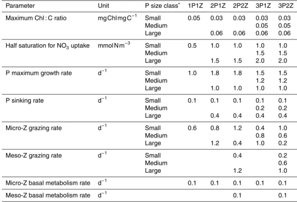
In this study five nitrogen-based marine ecosystem models were compared. All are

15

nitrogen-phytoplankton-zooplankton-detritus (NPZD) type models incorporating identi-cal biogeochemiidenti-cal processes (as described in Fennel et al., 2006), with the only dif-ference between models being the number of phytoplankton and zooplankton groups: 1P1Z, 2P1Z, 2P2Z and 3P1Z and 3P2Z food webs. The most complex 3P2Z model includes three P compartments (pico-, nano- and micro-phytoplankton) with three

cor-20

responding chlorophyll state variables and two Z compartments (micro- and meso-zooplankton). In the simplest 1P1Z model, the single P and Z compartments represent an average of three phytoplankton size classes and micro-zooplankton, respectively. In the 2P models, one phytoplankton compartment represents the micro-phytoplankton and one represents an average of pico- plus nano-phytoplankton. The key

param-25

(6)

BGD

11, 481–520, 2014

Title Page

Tables Figures

◭ ◮

Back Close

Full Screen / Esc

Discussion

P

a

per

|

D

iscussion

P

a

per

|

Discussion

P

a

per

|

Discuss

ion

P

a

per

|

nutrient half-saturation constants, maximum growth rates and sinking rates, whereas Z compartments vary in grazing rates and food preference. Both micro- and meso-zooplankton were assumed to graze on all phytoplankton size classes but with varying grazing rates. This allowed micro-zooplankton to prefer pico- and nano-phytoplankton whereas meso-zooplankton preferred micro-phytoplankton. A summarized list of

criti-5

cal parameters for the various plankton state variables is provided in Table 1 and the biological equations are provided in the Appendix.

Each of the five marine ecosystem models were embedded in a 1-D (vertical) physi-cal model that contains standard parameterizations for vertiphysi-cal advection, diffusion and sinking particles that have been thoroughly described in a number of other 1-D

mod-10

eling studies (Friedrichs et al., 2007; Ward et al., 2010; Xiao and Friedrichs, 2014). Initial and bottom boundary conditions for the model state variables were set the same as in Xiao and Friedrichs (2014), i.e., provided by a corresponding three-dimensional (3-D) 1P1Z model implementation (Hofmann et al., 2008, 2011). Models with two size classes were initialized as one half of the 3-D 1P1Z concentrations, and models with

15

three size classes were initialized as one-third of these concentrations. Sensitivity ex-periments demonstrated that the 1-D models were not sensitive to these initial size fractionation ratios. In all experiments, carbon was derived by converting nitrogen (N) to carbon (C) via a constant Redfield C : N ratio and model estimates of particulate or-ganic carbon (POC) were computed as the sum of all phytoplankton, zooplankton and

20

detritus. All five models were run from 1 January 2004 through 31 December 2004 with a time step of 1 h.

2.2 Satellite-derived data

Based on the results of Xiao and Friedrichs (2014), three types of data were derived from the Sea-viewing Wide Field-of-view Sensor (SeaWiFS) and assimilated into the

25

(7)

BGD

11, 481–520, 2014

Title Page

Tables Figures

◭ ◮

Back Close

Full Screen / Esc

Discussion

P

a

per

|

D

iscussion

P

a

per

|

Discussion

P

a

per

|

Discuss

ion

P

a

per

|

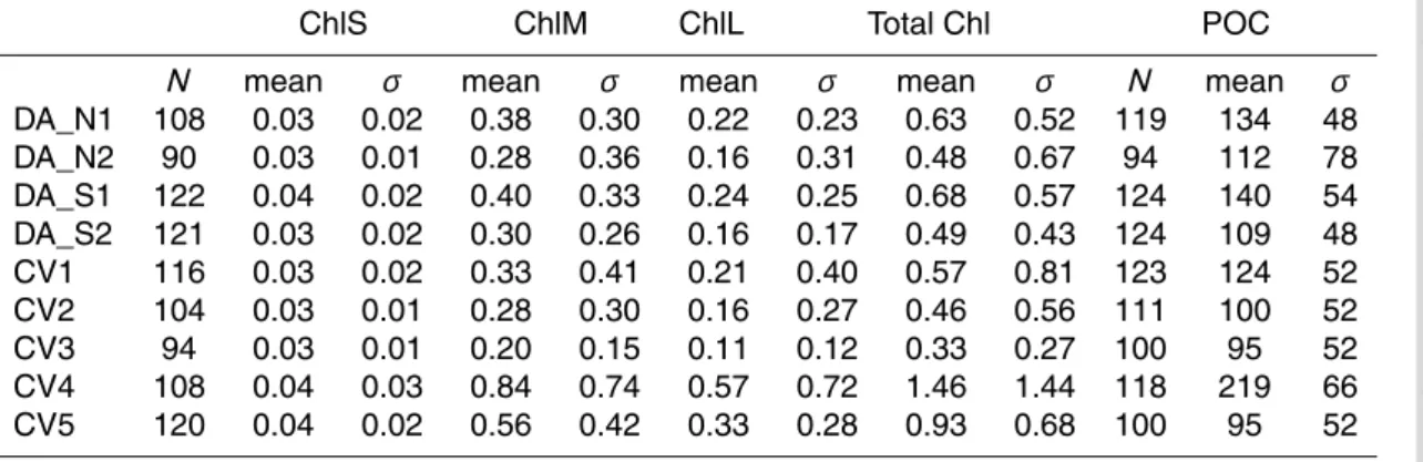
were all derived using empirical or semi-analytical algorithms, they have demonstrated considerable success in their agreement with in situ data. The uncertainty associated with these size-differentiated chlorophyll and POC concentrations have been estimated to be 35 % (Pan et al., 2010; Stramska and Stramski, 2005).

Satellite-derived fractionated chlorophyll consists of three types of

size-5

fractionated chlorophyll: large chlorophyll (ChlL), medium chlorophyll (ChlM) and small chlorophyll (ChlS), representing chlorophyll produced by micro-phytoplankton, nano-phytoplankton and pico-nano-phytoplankton, respectively. When comparing the models with two phytoplankton components to these satellite data, the chlorophyll attributed to the large phytoplankton component was compared to ChlL, and the chlorophyll attributed to

10

the small phytoplankton component was compared to the sum of ChlS+ChlM. When comparing the model with one phytoplankton component to these satellite data, the modeled chlorophyll was compared to the sum of all three types of chlorophyll. It is worth stressing that satellite measurements represent the first optical depth, which ac-counts for ∼90 % of the light exiting the ocean and towards space. In the MAB, the

15

depth range for this is from∼1 m within bay mouths/plumes to 20 m offshore, thus the

satellite data integrates the ocean’s surface layer and generally beyond the sea surface itself.

2.3 Data assimilation framework

The specifics of the optimization implementation are well documented in Xiao and

20

Friedrichs (2014), and thus only a brief description of the key properties of the vari-ational adjoint data assimilative framework are provided here.

The variational adjoint method is a nonlinear, weighted least-squares optimization method that minimizes the misfit between the model estimates and the observational data by optimizing a subset of model parameters (e.g., Lawson et al., 1995, 1996). The

25

(8)

assim-BGD

11, 481–520, 2014

Title Page

Tables Figures

◭ ◮

Back Close

Full Screen / Esc

Discussion

P

a

per

|

D

iscussion

P

a

per

|

Discussion

P

a

per

|

Discuss

ion

P

a

per

|

ilation results are obtained as long as data from multiple sites are assimilated, and the subset of parameters to be optimized include: maximum chlorophyll : carbon (Chl : C) ratios, maximum phytoplankton growth rates and zooplankton basal metabolism rates. Because each optimized parameter is size specific, i.e. each phytoplankton size class has a distinct Chl : C ratio and growth rate, and each zooplankton size class has a

dis-5

tinct basal metabolism rate (Table 1), the number of optimized parameters increases with increasing model complexity. For the five models tested here, 3, 5, 6, 7, and 8 parameters are optimized, respectively.

In this methodology the model-data misfit, otherwise known as the “cost function” (J), is minimized, where:

10

J₌ 1

M

K X

k=1

M X

m=1

1

Nkm·σ_km2 N_km X

j=1

(a_{j km}−aˆj km)2 (1)

wherearepresent the modeled equivalents to the observations ( ˆa),M is the number of data types whereM=2, 3, or 4 depending on the number of P size classes resolved by the model,K is the number of sites, N_km is the number of observations at site k 15

for data typem, andσkm is the standard deviation of theNkm observations (Table 2). In this way, the cost function provides an estimate of the ratio between the model-data differences and the differences between the data and the mean of the data, i.e.σ_km2 .

After the cost function is computed from an a priori forward model run, the adjoint code (Giering and Kaminski, 1998) computes the gradients of the cost function and

20

passes the information to an optimization procedure (Gilbert and Lemaréchal, 1989), which determines how each optimized parameter value should be modified in order to reduce the magnitude of the cost function. The new parameter values are then used in another forward model run, the new cost function is computed, and the optimiza-tion procedure is repeated. These iteraoptimiza-tions continue until the specified convergence

25

criterion is satisfied.

(9)

previ-BGD

11, 481–520, 2014

Title Page

Tables Figures

◭ ◮

Back Close

Full Screen / Esc

Discussion

P

a

per

|

D

iscussion

P

a

per

|

Discussion

P

a

per

|

Discuss

ion

P

a

per

|

ous study found that POC estimates were not significantly improved as a result of the assimilation, the POC assimilation played a critical role in preventing significant deteri-oration of other state variables (zooplankton, detritus) that are included as components of POC. Thus the cost that was minimized by the optimization routine consists of the sum of these two components:

5

Size_cost₌SizeChl_cost₊POC_cost (2)

where SizeChl_cost represents that portion of the cost due to the model-data misfits of size differentiated chlorophyll, and POC_cost represents the portion of the cost due to the POC model-data misfits. For the 1P model, SizeChl_cost is computed for total

10

chlorophyll (ChlS₊ChlM₊ChlL) and thus M₌2 in Eq. (1) (i.e. one data type is total ChlS+ChlM+ChlL and one is POC.) For the 2P models, SizeChl_cost is computed as the sum of two separate components: ChlS+ChlM and ChlL. In this case M=3 (data types are ChlS₊ChlM, ChlL and POC.) Finally, for the 3P models, SizeChl_cost includes misfits for ChlS, ChlM and ChlL separately, and four data types are assimilated

15

(M=4; ChlS, ChlM, ChlL, and POC.)

As a result of the nonlinearities in the cost function formulation (Eq. 1), SizeChl_cost is not comparable across models with different numbers of phytoplankton variables, and thus Size_cost is not an appropriate metric for comparing the relative skill of all five models. Thus it is also critical to compute and compare the total cost (Total_cost)

20

from the misfits in total chlorophyll and POC for the five models:

Total_cost=TotChl_cost+POC_cost (3)

where TotChl_cost represents the model-data misfits in total chlorophyll concentration. (Note that for the model with a single phytoplankton size class Total_cost=Size_cost,

25

since in this case the size fractionated chlorophyll is identically equal to the total chloro-phyll.) In this way, although for four of the five models Total_cost does not precisely correspond to the cost that is minimized through the optimization process, it provides a standard metric that can be used to rigorously compare the relative skill of all five ecosystem models.

(10)

BGD

11, 481–520, 2014

Title Page

Tables Figures

◭ ◮

Back Close

Full Screen / Esc

Discussion

P

a

per

|

D

iscussion

P

a

per

|

Discussion

P

a

per

|

Discuss

ion

P

a

per

|

2.4 Model implementation and assimilation experiments

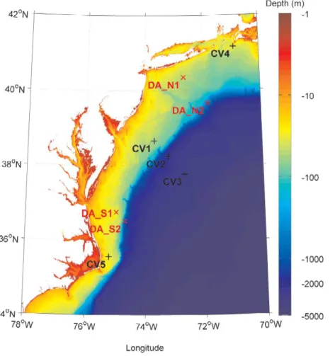
The five ecosystem models were implemented in the framework described above at nine locations in the Mid-Atlantic Bight (Fig. 1). Four of these sites were designated as “Data Assimilation” (DA) sites, since these are the locations at which data were assimilated. The remaining five sites were designated as “Cross Validation” (CV) sites,

5

since these were sites where the optimal parameters derived from assimilating data at the DA sites were independently tested. Three experiments were conducted at these nine sites, and are described in more detail below.

Expt. 1. Each model was implemented in a forward model run at all nine sites, and a priori cost functions (both Size_cost and Total_cost) from these pre-assimilation

sim-10

ulations were computed.

Expt. 2. POC data and size fractionated chlorophyll data from the four DA sites were assimilated into each of the five models to determine a single best-fit set of parameter values for these four sites. The resulting cost functions (both Size_cost and Total_cost) were computed both at the four DA sites, as well as at the five CV sites.

15

Expt. 3. To determine the robustness of the optimal parameters determined in Expt. 2 and the sensitivity of these parameter values to uncertainties associated with the satellite-derived products, normally distributed random noise with a maximum ampli-tude of 20 % was added to the size fractionated chlorophyll and POC data from the four DA sites prior to assimilation. The resulting optimal parameter values were

com-20

(11)

BGD

11, 481–520, 2014

Title Page

Tables Figures

◭ ◮

Back Close

Full Screen / Esc

Discussion

P

a

per

|

D

iscussion

P

a

per

|

Discussion

P

a

per

|

Discuss

ion

P

a

per

|

3 Results

3.1 Expt. 1: a priori simulation

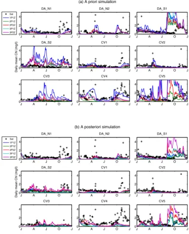
All five a priori surface chlorophyll simulations from the five di_fferent models were com-parable at most of the nine sites, in particular at the northern sites such as N1, N2, CV1 and CV2 (Fig. 2a). More variability between models was found at the southern

5

sites and o_ffshore sites. For example, the model estimates of the peak chlorophyll dur-ing the Fall bloom ranged from 2 mg Chl m−3_{(the 2P1Z model) to}_>_{5 mg Chl m}−3 _(the 3P2Z model) at the CV5 site. The 1P1Z model stood out from the other four models in that it tended to produce slightly higher chlorophyll concentrations at most of the sites, while it still gave similar estimates on the bloom timing as the other models (Fig. 2a).

10

In terms of size-fractions (not shown), the simulations generated by the 2P and the 3P models also resembled one another at most sites. For example, at all nine sites ChlL concentrations remained low (<10 % of total chlorophyll) for most of the year except during the spring and fall blooms. For the 3P models, model estimates of ChlM were also considerably lower than ChlS throughout the year at all nine sites. For all 2P

15

and 3P models, ChlS was the dominant chlorophyll component throughout most of the year.

Although all models failed to capture some key features of the surface chlorophyll dis-tributions (Fig. 2a) such as bloom timing (e.g. at site DA_S1) and magnitude (e.g. at site DA_N2), in general, all five models fit the satellite-derived surface total chlorophyll and

20

POC distributions similarly well. The general consistency in the five model simulations resulted in the a priori cost functions of the five models being relatively comparable. At both the DA sites (Table 3) and the CV sites (Table 4) the a priori Total_cost was highest for the simplest 1P1Z model, primarily as a result of an overestimate of surface chlorophyll at the DA_S2 site and the offshore CV3 site (Fig. 2a). The 3P models

per-25

(12)

BGD

11, 481–520, 2014

Title Page

Tables Figures

◭ ◮

Back Close

Full Screen / Esc

Discussion

P

a

per

|

D

iscussion

P

a

per

|

Discussion

P

a

per

|

Discuss

ion

P

a

per

|

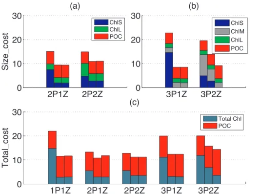
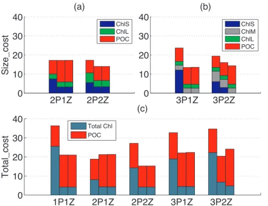
a second zooplankton component (Tables 3, 4). In terms of the 3P models, the model with the second zooplankton component produced slightly lower a priori Size_costs.

3.2 Expt. 2: assimilation of satellite-derived data

3.2.1 Expt. 2 results at Data Assimilation (DA) sites

The assimilation of size differentiated chlorophyll and POC data at the four DA sites

5

resulted in significant reductions in Size_cost (Table 3) indicating successful optimiza-tions for all five models. Improvements in model-data misfit were most substantial at the two southern stations (DA_S1 and DA_S2) (Fig. 2b). As expected from the previ-ous results of Xiao and Friedrichs (2014) this reduction in Size_cost was accomplished primarily through improvements in chlorophyll model-data fit (Fig. 3a and b). The

assim-10

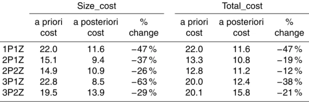
ilation particularly improved model-data misfit for the smallest size class of chlorophyll for all five models. The 2Z models also produced improved model-data fits for other size classes of chlorophyll, but this was not the case for the 1Z models.

Although Size_cost cannot be used to quantitatively compare the skill of all five mod-els (see Sect. 2.3), it is still a useful metric for comparison of modmod-els with the same

15

numbers of phytoplankton variables. Somewhat surprisingly, Size_cost was lower (and percent reduction in cost much greater) for models with only one zooplankton size class, than for those with two zooplankton size classes. This effect was stronger for the more complex 3P models than for the 2P models (Table 3).

In order to compare models with different phytoplankton structures, Total_cost was

20

computed to represent the model-data misfits of total chlorophyll and POC (Table 3; Fig. 3c). After assimilation, Total_cost decreased for all models (mean decrease of

∼30 %), which was only slightly smaller than the analogous decrease of Size_cost

(mean decrease of∼40 %). The lowest a posteriori costs were found with the simplest

1P and 2P models, and the highest cost was obtained using the most complex 3P2Z

25

(13)

BGD

11, 481–520, 2014

Title Page

Tables Figures

◭ ◮

Back Close

Full Screen / Esc

Discussion

P

a

per

|

D

iscussion

P

a

per

|

Discussion

P

a

per

|

Discuss

ion

P

a

per

|

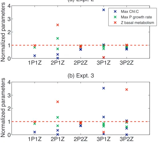
Optimal parameters generated by the five models were all well constrained (Fig. 4a). Out of the 29 optimized parameters for the five models, only seven of these represented a change of greater than 50 %. Both 2Z models showed only minor changes in param-eter values, whereas the three 1Z models all had at least one paramparam-eter that changed by more than 50 %. The large changes in parameter values for these 1Z models are

5

consistent with the largest reductions in costs for these models, as discussed above. However, the 2P2Z model fit the total chlorophyll data (Total_cost=11.2) nearly as well as the 2P1Z model (Total_cost=10.8), despite much smaller changes to the a priori parameter values. Specifically, the superior fit of the 2P1Z model was obtained only when the maximum Chl : C ratio for micro-phytoplankton was unrealistically reduced

10

by an order of magnitude.

Among the three types of optimized parameters, the maximum phytoplankton growth rate was adjusted the least by the optimization, suggesting that these parameters were initialized near their optimal values. Greater variations in optimal values were found with the other parameters, without any clear patterns forming as a function of model

15

structure.

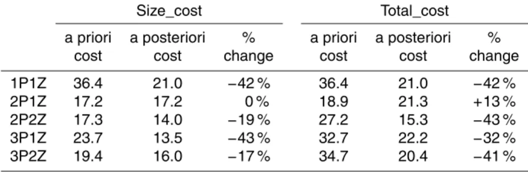
3.2.2 Expt. 2 results at Cross Validation (CV) sites

By definition, the data assimilation improved model skill at the DA sites (Table 3) where the data were assimilated; however a more robust test of the optimization is to evaluate the optimized models against data at the CV sites (Table 4) where no data were

assimi-20

lated (Gregg et al., 2009). When the optimal parameter sets obtained from assimilating the data at the DA sites were applied to another five nearby sites (CV sites in Fig. 1), Size_cost was reduced for all models except the 2P1Z model (Table 4, Fig. 5a and b). The greatest reductions in Size_cost at the CV sites occurred for the 3P1Z and 1P1Z models (∼40 %), which was equivalent to the reductions in Size_cost generated by

25

these models at the DA sites. Significant, but smaller, reductions also occurred for the 2P2Z and 3P2Z models (∼20 %; Table 4). All five models showed an increase in

(14)

chloro-BGD

11, 481–520, 2014

Title Page

Tables Figures

◭ ◮

Back Close

Full Screen / Esc

Discussion

P

a

per

|

D

iscussion

P

a

per

|

Discussion

P

a

per

|

Discuss

ion

P

a

per

|

phyll, particularly for the smallest chlorophyll size class, more than compensated for the deterioration in POC model-data misfit in all cases except for the 2P1Z model (Fig. 5a and b).

Applying the optimal parameters from the DA sites to simulations at the CV sites also generated significant improvements in the total chlorophyll cost for each of the

5

five models (Fig. 5c). This decrease in total chlorophyll cost was again substantially larger than the increase in POC cost for all models except the 2P1Z model, and thus the overall Total_cost also decreased for four of the five models (Table 4). The lack of improvement for the 2P1Z model is at least partially due to the fact that using the a priori parameter values with the 2P1Z model generated an a priori simulation that

10

fit the data at the five CV sites very well (Fig. 5c). In fact the a priori Total_cost for the 2P1Z model was lower than the a posteriori Total_cost of the 1P and 3P models (Table 4, Fig. 5c). Overall, the intermediately complex 2P2Z model produced the lowest Total_cost when using the parameters optimized for the DA sites at the CV sites.

3.3 Expt. 3: assimilation of perturbed data

15

3.3.1 Expt. 3 results at Data Assimilation (DA) sites

The a priori costs for Expt. 3 were computed as the difference between the a priori simulations and the noisy data, and were only very slightly different (<1 %) from the a priori costs for Expt. 2, which were computed as the difference between the a priori simulations and the actual data.

20

When the noisy data were assimilated into the models at the four DA sites in Expt. 3, the optimization process generated very similar parameters to those generated in Expt. 2 for the 1P, 2P and 3P1Z models (Fig. 4). Thus the addition of random noise did not significantly affect the optimization process for these simpler models, and as a result the a posteriori Size_costs resulting from the assimilation of the noisy data were almost

25

(15)

BGD

11, 481–520, 2014

Title Page

Tables Figures

◭ ◮

Back Close

Full Screen / Esc

Discussion

P

a

per

|

D

iscussion

P

a

per

|

Discussion

P

a

per

|

Discuss

ion

P

a

per

|

In contrast, the optimal parameters generated in Expt. 3 for the most complex 3P2Z model were significantly different from those in Expt. 2 (Fig. 4b). For example, the op-timal value for the maximum Chl : C ratio for pico-phytoplankton in the 3P2Z model was 6.1×10−13mg Chl mg C−1 compared to a value of 0.023 generated when

assim-ilating the actual satellite-derived data. As a result, this new set of optimal parameter

5

values (Fig. 4b) resulted in a significantly different Size_cost (∼35 % decrease). This

decrease in the 3P2Z Size_cost was caused by a substantial reduction in the cost com-ponents of ChlS and ChlM, whereas the contribution of ChlL and POC remained nearly unchanged (Fig. 3b).

3.3.2 Expt. 3 results at Cross Validation (CV) sites

10

The costs at the CV sites for the 1P, 2P and 3P1Z models were nearly identical for Expt. 2 and 3 (Fig. 5). This was true despite some significant changes in the optimized parameter values for the 3P1Z model (Fig. 4), e.g., the zooplankton basal metabolism rate was twice as high in Expt. 3 compared to Expt 2. As was the case at the DA sites, the 3P2Z a posteriori costs were much more sensitive to the noise added to the

15

data prior to assimilation. Although the a posteriori 3P2Z Size_cost decreased for the ChlS and ChlM components, the a posteriori Total_cost increased due to a significant deterioration in the model-data fit for POC.

In summary, the addition of noise to the assimilated data had almost no effect on the cost functions for the simpler models, but significantly affected the costs of the most

20

(16)

BGD

11, 481–520, 2014

Title Page

Tables Figures

◭ ◮

Back Close

Full Screen / Esc

Discussion

P

a

per

|

D

iscussion

P

a

per

|

Discussion

P

a

per

|

Discuss

ion

P

a

per

|

4 Discussion and conclusions

In this study, five lower trophic level ecosystem models with varying food web complex-ities were rigorously compared, in order to determine how the number of phytoplank-ton and zooplankphytoplank-ton compartments a_ffects the ability of a lower trophic level model to reproduce observed patterns in surface chlorophyll and particulate organic carbon.

5

All five models were embedded in a 1-D assimilative model framework with identical physics and biogeochemical formulations, and thus the differences in the model sim-ulations were only a result of variations in the complexity of the planktonic food web structure.

As expected based on previous studies assimilating satellite-derived data fields into

10

marine ecosystem models (Fan and Lv, 2009; Friedrichs, 2002; Garcia-Gorriz et al., 2003; Hemmings et al., 2004; Tjiputra et al., 2007), all models tested here showed improvement in model skill after the assimilation of the satellite-derived fields and re-sulting optimization of the plankton-related parameters. Whereas prior to assimilation the five models varied somewhat in their ability to fit the satellite-derived data fields,

15

after assimilation the models produced total chlorophyll and POC fields at the assimi-lation sites that matched the satellite data nearly equally well.

Interestingly, the a posteriori parameters optimized for these five models were very different for the different models. In particular, the models with a single zooplankton size class were only able to reproduce the assimilated data using extremely low zooplankton

20

basal metabolism rates, or extremely low maximum Chl : C ratios, whereas the models with two zooplankton size classes were able to reproduce the POC and chlorophyll observations using realistic rates and ratios. Ultimately, the parameters optimized for the two phytoplankton, two zooplankton (2P2Z) model were most similar to our best-guess a priori initial parameter values.

25

(17)

BGD

11, 481–520, 2014

Title Page

Tables Figures

◭ ◮

Back Close

Full Screen / Esc

Discussion

P

a

per

|

D

iscussion

P

a

per

|

Discussion

P

a

per

|

Discuss

ion

P

a

per

|

improved the simulations at a number of other sites throughout the region, giving us confidence in the portability of these optimized parameter values, and optimism for the potential success of using these parameters in a three-dimensional simulation of the US eastern continental shelf (McDonald et al., 2012). Although almost all models showed some degree of improvement at these other MAB sites, once again the model

5

characterized by intermediate complexity, i.e. 2P2Z, performed best. The other models were able to fit the data at the assimilation sites equally as well as the 2P2Z model; however, they typically did so by using unrealistic parameter values which were not portable to other areas of the Mid-Atlantic Bight.

Intriguing results were also obtained when random noise was added to the

satellite-10

derived data prior to assimilation. The addition of the noise perturbation had almost no effect on the values of the optimized parameters for the simplest four models, suggest-ing that the optimization process was robust for these models, even when significant noise was present in the assimilated data. On the contrary, when these perturbed data were assimilated into the most complex model (the 3P2Z model), substantially different

15

optimal parameter values were obtained. For certain parameters (e.g., the maximum Chl : C ratio for pico-phytoplankton), the di_fference between the optimized parameter values obtained by assimilating the actual data vs. those obtained by assimilating the noisy data was more than ten orders of magnitude. Although the new parameter val-ues obtained by assimilating the noisy data improved the model-data fit at the specific

20

sites where the data were assimilated, the unrealistic parameter values deteriorated the model performance at other sites within the MAB. In essence, unlike the simpler models, the most complex model had enough flexibility that it was actually able to fit the additional noise artificially added to the data. Although this “over-tuning” actually improved the model-data fit at the sites where the noisy data were assimilated, this is

25

a dangerous outcome, as the model-data fit was degraded at other locations within the MAB where data were not available for assimilation.

(18)

BGD

11, 481–520, 2014

Title Page

Tables Figures

◭ ◮

Back Close

Full Screen / Esc

Discussion

P

a

per

|

D

iscussion

P

a

per

|

Discussion

P

a

per

|

Discuss

ion

P

a

per

|

and cross-validated the resulting optimal parameters against the data in the remaining season. Their cross-validation experiments showed that complex models with too many unconstrained parameters might be able to fit the assimilated data extremely well (the more free parameters the better the fit to the assimilated data), yet these complex models would have poor predictive ability (the more free parameters the worse the fit

5

to independent, unassimilated data).

Another difficulty with complex models is that they are usually governed by such a large number of parameters (the number of parameters that must be specified in a given ecosystem model generally increases by as much as the square of the number of state variables, Denman, 2003), that it is very difficult to identify the best-fit set of

pa-10

rameters. When hand-tuning such models, there are just too many different parameters to adequately test all parameter combinations. When applying an automated parame-ter optimization method such as the variational adjoint method to complex models with multiple unconstrained parameters, the cost function has a tendency to get stuck in suboptimal “local minima” and as a result the absolute global cost function minimum

15

and the true “best-fit” set of parameters potentially can never be identified. In fact, this is exactly what occurred in the present study for the most complex 3P2Z model. The a posteriori cost function was highest for this model, despite the presumably increased flexibility that this model had to fit the data, because the cost function became stuck in a local minimum. However, when artificial noise was added to the data prior to

as-20

similation, an alternate local cost function minimum was identified, which, somewhat surprisingly, was smaller than the one identified when the true data were assimilated. The problem of complex models becoming stuck in local cost function minima has also been discussed by others. For example, Ward et al. (2010) demonstrated that when too many unconstrained parameters were optimized, the cost function often became

25

trapped in a local minimum; however, reducing the number of optimized parameters partially eliminated this problem.

(19)

BGD

11, 481–520, 2014

Title Page

Tables Figures

◭ ◮

Back Close

Full Screen / Esc

Discussion

P

a

per

|

D

iscussion

P

a

per

|

Discussion

P

a

per

|

Discuss

ion

P

a

per

|

types of models without the formal parameter optimization techniques employed here. For example, an early study by Costanza and Sklar (1985) rated eighty-seven models in wetland and shallow water bodies in terms of three indices: articulation (the complex-ity of the model), accuracy (goodness-of-fit of the model to the data) and effectiveness (trade-offbetween complexity and accuracy). They concluded that although the

accu-5

racy seemed to increase with articulation, the maximum effectiveness was found at an intermediate level of complexity. Fulton et al. (2003) found a similar humped relation-ship between model complexity and performance when examining end-to-end (nutrient to fisheries) models, demonstrating that the best performance was produced by the model with intermediate complexity. Another model comparison study was conducted

10

by Raick et al. (2006), in which three simplified pelagic ecosystem models with sixteen, nine and four state variables, respectively, were assessed according to their ability to reproduce simulations from performance of a complex model with nineteen state vari-ables. The study found that although the simplest model (four state variables) was able to capture the key features demonstrated by the complex model, the model with

inter-15

mediate complexity (nine state variables) most closely reproduced the output from the full 19 state-variable model.

In summary, the study presented here provides additional evidence that lower trophic level food web models of intermediate complexity (e.g. containing two phytoplankton and two zooplankton compartments) are most likely to be able to provide best

esti-20

mates of chlorophyll and carbon concentrations on regional scales such as the US eastern continental shelf. Simple models with only a single zooplankton size class may be able to reproduce observed data fields, but typically can only do so using unrealistic parameters that are not portable throughout the region. On the contrary, more complex models have difficulty finding cost minima and have issues with over-tuning and

artifi-25

(20)

BGD

11, 481–520, 2014

Title Page

Tables Figures

◭ ◮

Back Close

Full Screen / Esc

Discussion

P

a

per

|

D

iscussion

P

a

per

|

Discussion

P

a

per

|

Discuss

ion

P

a

per

|

Appendix A

Model equations

The equations for each of the five models are included below for reference. In each case, the specific equations for phytoplankton growth rate (µ), zooplankton grazing rate (g), nitrification rate (n) and the variable ratio of chlorophyll to

phy-5

toplankton biomass (Chl) are provided in Fennel et al. (2006). State variables are defined as: P=total phytoplankton, Z=total zooplankton, SD=small detritus, LD=large detritus, NO3=nitrate, NH4=ammonium, Chl=chlorophyll, SP=small phy-toplankton, MP=medium phytoplankton, LP=large phytoplankton, SZ=small zoo-plankton, MZ=medium zooplankton, LZ=large zooplankton, ChlS=small chlorophyll,

10

(21)

BGD

11, 481–520, 2014

Title Page

Tables Figures

◭ ◮

Back Close

Full Screen / Esc

Discussion

P

a

per

|

D

iscussion

P

a

per

|

Discussion

P

a

per

|

Discuss

ion

P

a

per

|

Functional formulations (example for SP, SZ)

g_{SP_SZ}₌g_{max_SP_SZ} SP

2

kP+SP

2

ρChlS=

θmax_SPµSP·SP

αI·ChlS

fSP(I)=

αI

q

µ2_{max_SP}₊α2_I2

LNO3_SP=

NO3

kNO3_SP+NO3

1+NH4

kNH4

−1

5

L_NH4= NH4

k_NH4+NH4

µSP=µmax_SPfSP(I)(LNO3_SP+LNH4)

µ_{SP_NO3}=µ_{max_SP}f_SP(I)L_{NO3_SP} µSP_NH4=µmax_SPfSP(I)LNH4

(22)

BGD

11, 481–520, 2014

Title Page

Tables Figures

◭ ◮

Back Close

Full Screen / Esc

Discussion

P

a

per

|

D

iscussion

P

a

per

|

Discussion

P

a

per

|

Discuss

ion

P

a

per

|

1P1Z (includes P, Z)

∂P

∂t =µPP−gP_ZZ−mPP−τ(SD+P)P−wP

∂P

dz

∂Z

∂t =gP_ZβZ−lBM_ZZ−lE

P2

kP+P2

βZ−mZZ2

∂SD

∂t =gP_Z(1−β)Z+mZZ

2

+m_PP−τ(SD+P)SD−rSDSD−wSD

∂SD

∂z

∂LD

∂t =τ(SD+P)

2

−rLDLD−wLD

∂LD

∂z 5

∂NO3

∂t =−µP_NO3P+nNH4

∂NH4

∂t =−µP_NH4P−nNH4+lBM_ZZ+lE

P2

k_P₊P2βZ+rSDSD+rLDLD

∂Chl

∂t =ρChlµPChl−gP_ZZ

Chl

(23)

BGD

11, 481–520, 2014

Title Page

Tables Figures

◭ ◮

Back Close

Full Screen / Esc

Discussion

P

a

per

|

D

iscussion

P

a

per

|

Discussion

P

a

per

|

Discuss

ion

P

a

per

|

2P1Z (includes SP, LP, Z)

∂SP

∂t =µSPSP−gSP_ZZ−mPSP−τ(SD+P)SP−wSP

∂SP

dz

∂LP

∂t =µLPLP−gLP_ZZ−mPLP−τ(SD+P)LP−wLP

∂LP

dz

∂Z

∂t =(gSP_Z+gLP_Z)βZ−lBM_ZZ−lE

P2

k_P+P2βZ−mZZ 2

∂SD

∂t =(gSP_Z+gLP_Z)(1−β)Z+mZZ

2

+mPP−τ(SD+P)SD−rSDSD−wSD

∂SD

∂z 5

∂LD

∂t =τ(SD+P)

2

−rLDLD−wLD

∂LD

∂z

∂NO3

∂t =−µSP_NO3SP−µLP_NO3LP+nNH4

∂NH4

∂t =−µSP_NH4SP−µLP_NH4LP−nNH4+lBM_ZZ+lE

P2

kP+P2

βZ+r_SDSD+r_LDLD

∂ChlS

∂t =ρChlSµSPChlS−gSP_ZZ

ChlS

SP −mPChlS−τ(SD+P)ChlS

∂ChlL

∂t =ρChlLµLPChlL−gLP_ZZ

ChlL

(24)

BGD

11, 481–520, 2014

Title Page

Tables Figures

◭ ◮

Back Close

Full Screen / Esc

Discussion

P

a

per

|

D

iscussion

P

a

per

|

Discussion

P

a

per

|

Discuss

ion

P

a

per

|

2P2Z (includes SP, LP, SZ, LZ)

∂SP

∂t =µSPSP−gSP_SZSZ−gSP_LZLZ−mPSP−τ(SD+P)SP−wSP

∂SP

dz

∂LP

∂t =µLPLP−gLP_SZSZ−gLP_LZLZ−mPLP−τ(SD+P)LP−wLP

∂LP

dz

∂SZ

∂t =(gSP_SZ+gLP_SZ)βSZ−lBM_SZSZ−lE

P2

k_P+P2βSZ−mZSZ

2

∂LZ

∂t =(gSP_LZ+gLP_LZ)βLZ−lBM_LZLZ−lE

P2

k_P₊P2βLZ−mZLZ 2

5

∂SD

∂t =(gSP_SZ+gLP_SZ)(1−β)SZ+(gSP_LZ+gLP_LZ)(1−β)LZ+mZSZ

2

+mZLZ2

+mPP−τ(SD+P)SD−rSDSD−wSD

∂SD

∂z

∂LD

∂t =τ(SD+P)

2

−rLDLD−wLD

∂LD

∂z

∂NO3

∂t =−µSP_NO3P−µLP_NO3P+nNH4

∂NH4

∂t =−µSP_NH4P−µLP_NH4P−nNH4+lBM_SZSZ+lBM_LZLZ+lE

P2

kP+P2

βZ

10

+r_SDSD+r_LDLD

∂ChlS

∂t =ρChlSµSPChlS−gSP_SZSZ

ChlS

SP −gSP_LZLZ

ChlS

∂ChlL

∂t =ρChlLµLPChlL−gLP_SZSZ

ChlL

LP −gLP_LZLZ

ChlL

(25)

BGD

11, 481–520, 2014

Title Page

Tables Figures

◭ ◮

Back Close

Full Screen / Esc

Discussion

P

a

per

|

D

iscussion

P

a

per

|

Discussion

P

a

per

|

Discuss

ion

P

a

per

|

3P1Z (includes SP, MP, LP, Z)

∂SP

∂t =µSPSP−gSP_ZZ−mPSP−τ(SD+P)SP−wSP

∂SP

dz

∂MP

∂t =µMPMP−gMP_ZZ−mPMP−τ(SD+P)MP−wMP

∂MP

dz

∂LP

∂t =µLPLP−gLP_ZZ−mPLP−τ(SD+P)LP−wLP

∂LP

dz

∂Z

∂t =(gSP_Z+gMP_Z+gLP_Z)βZ−lBM_ZZ−lE

P2

kP+P2

βZ−mZZ2

5

∂SD

∂t =(gSP_Z+gMP_Z+gLP_Z)(1−β)Z+mZZ

2

+mPP−τ(SD+P)SD−rSDSD

−wSD

∂SD

∂z

∂LD

∂t =τ(SD+P)

2

−rLDLD−wLD

∂LD

∂z

∂NO3

∂t =−µSP_NO3P−µMP_NO3P−µLP_NO3P+nNH4

∂NH4

∂t =−µSP_NH4P−µMP_NH4P−µLP_NH4P−nNH4+lBM_ZZ 10

+lE

P2

k_P+P2βZ+rSDSD+rLDLD

∂ChlS

∂t =ρChlSµSPChlS−gSP_ZZ

ChlS

∂ChlM

∂t =ρChlMµMPChlM −gMP_ZZ

ChlM

MP −mPChlM −τ(SD+P)ChlM

∂ChlL

∂t =ρChlLµLPChlL−gLP_ZZ

ChlL

LP −mPChlL−τ(SD+P)ChlL

(26)

BGD

11, 481–520, 2014

Title Page

Tables Figures

◭ ◮

Back Close

Full Screen / Esc

Discussion

P

a

per

|

D

iscussion

P

a

per

|

Discussion

P

a

per

|

Discuss

ion

P

a

per

|

3P2Z (includes SP, MP, LP, SZ, LZ)

∂SP

∂t =µSPSP−gSP_SZSZ−gSP_LZLZ−mPSP−τ(SD+P)SP−wSP

∂SP

dz

∂MP

∂t =µMPMP−gMP_SZSZ−gMP_LZLZ−mPMP−τ(SD+P)MP−wMP

∂MP

dz

∂LP

∂t =µLPLP−gLP_SZSZ−gLP_LZLZ−mPLP−τ(SD+P)LP−wLP

∂LP

dz

∂SZ

∂t =(gSP_SZ+gMP_SZ+gLP_SZ)βSZ−lBM_SZSZ−lE

P2

k_P₊P2βSZ−mZSZ

2

5

∂LZ

∂t =(gSP_LZ+gMP_LZ+gLP_LZ)βLZ−lBM_LZLZ−lE

P2

kP+P2

βLZ−mZLZ2

∂SD

∂t =(gSP_SZ+gMP_SZ+gLP_SZ)(1−β)SZ+(gSP_LZ+gMP_LZ+gLP_LZ)(1−β)LZ

+mZSZ2+mZLZ2+mPP−τ(SD+P)SD−rSDSD−wSD

∂SD

∂z

∂LD

∂t =τ(SD+P)

2

−rLDLD−wLD

∂LD

∂z

∂NO3

∂t =−µSP_NO3P−µMP_NO3P−µLP_NO3P+nNH4 10

∂NH4

∂t =−µSP_NH4P−µMP_NH4P−µLP_NH4P−nNH4+lBM_SZSZ+lBM_LZLZ

+lE

P2

kP+P2

βZ+rSDSD+rLDLD

∂ChlS

∂t =ρChlSµSPChlS−gSP_SZSZ

ChlS

SP −gSP_LZLZ ChlS

SP

−mPChlS−τ(SD+P)ChlS

(27)

BGD

11, 481–520, 2014

Title Page

Tables Figures

◭ ◮

Back Close

Full Screen / Esc

Discussion

P

a

per

|

D

iscussion

P

a

per

|

Discussion

P

a

per

|

Discuss

ion

P

a

per

|

∂ChlM

∂t =ρChlMµMPChlM−gMP_SZSZ

ChlS

MP −gMP_LZLZ ChlM

MP

−mPChlM −τ(SD+P)ChlM

∂ChlL

∂t =ρChlLµLPChlL−gLP_SZSZ

ChlL

LP −gLP_LZLZ ChlL

LP −mPChlL−τ(SD+P)ChlL

Acknowledgements. This work was supported by the NASA Earth and Space Science

Fel-5

lowship Program (Grant NNX10AN50H) and the NASA Interdisciplinary Science Program (NNX11AD47G). The authors are grateful to the NASA US Eastern Continental Shelf Carbon Cycling (USECoS) team for their useful comments, especially Kimberly Hyde, Antonio Mannino and Xiaoju Pan for providing the satellite-derived size-fractionated chlorophyll data. The authors would like to thank the SeaWiFS Project (Code 970.2) and the Distributed Active Archive

Cen-10

ter (Code 610.2) at the Goddard Space Flight Center, Greenbelt, MD 20771, for the production and distribution of these data, respectively. This is VIMS contribution # 3342.

References

Anderson, T. R.: Plankton functional type modelling: running before we can walk?, J. Plankton Res., 27, 1073–1081, doi:10.1093/plankt/fbi076, 2005.

15

Baird, M. E. and Suthers, I. M.: Increasing model structural complexity inhibits the growth of ini-tial condition errors, Ecol. Complex., 7, 478–486, doi:10.1016/j.ecocom.2009.12.001, 2010. Bagniewski, W., Fennel, K., Perry, M. J., and D’Asaro, E. A.: Optimizing models of the North

At-lantic spring bloom using physical, chemical and bio-optical observations from a Lagrangian float, Biogeosciences, 8, 1291–1307, doi:10.5194/bg-8-1291-2011, 2011.

20

Costanza, R. and Sklar, F. H.: Articulation, accuracy and effectiveness of mathematical mod-els: a review of freshwater wetland applications, Ecol. Model., 27, 45–68, doi:10.1016/0304-3800(85)90024-9, 1985.

Denman, K. L.: Modelling planktonic ecosystems: parameterizing complexity, Prog. Oceanogr., 57, 429–452, 2003.

25

(28)

BGD

11, 481–520, 2014

Title Page

Tables Figures

◭ ◮

Back Close

Full Screen / Esc

Discussion

P

a

per

|

D

iscussion

P

a

per

|

Discussion

P

a

per

|

Discuss

ion

P

a

per

|

Fennel, K., Wilkin, J., Levin, J., Moisan, J., O’Reilly, J., and Haidvogel, D.: Nitrogen cycling in the Middle Atlantic Bight: results from a three-dimensional model and implications for the North Atlantic nitrogen budget, Global Biogeochem. Cy., 20, GB3007, doi:10.1029/2005gb002456, 2006.

Fennel, K., Wilkin, J., Previdi, M., and Najjar, R.: Denitrification effects on air-sea CO₂flux in

5

the coastal ocean: Simulations for the northwest North Atlantic, Geophys. Res. Lett., 35, L24608, doi:10.1029/2008gl036147, 2008.

Flynn, K. J.: Castles built on sand: dysfunctionality in plankton models and the inadequacy of dialogue between biologists and modellers, J. Plankton Res., 27, 1205–1210, 2005.

Follows, M. J., Dutkiewicz, S., Grant, S., and Chisholm, S. W.: Emergent

bio-10

geography of microbial communities in a model ocean, Science, 315, 1843–1846, doi:10.1126/science.1138544, 2007.

Friedrichs, M. A. M.: The assimilation of SeaWiFS and JGOFS EqPac data into a marine ecosystem model of the central equatorial Pacific, Deep-Sea Res. Pt. II, 49, 289–319, 2002. Friedrichs, M. A. M., Dusenberry, J., Anderson, L., Armstrong, R., Chai, F., Christian, J.,

15

Doney, S. C., Dunne, J., Fujii, M., Hood, R., McGillicuddy, D., Moore, K., Schartau, M., Spitz, Y. H., and Wiggert, J.: Assessment of skill and portability in regional marine biogeo-chemical models: role of multiple phytoplankton groups, J. Geophys. Res., 112, C08001, doi:10.1029/2006JC003852, 2007.

Friedrichs, M. A. M., Hood, R. R., and Wiggert, J. D.: Ecosystem model complexity vs. physical

20

forcing: Quantification of their relative impact with assimilated Arabian Sea data, Deep-Sea Res. Pt. II, 53, 576–600, doi:10.1016/j.dsr2.2006.01.026, 2006.

Friedrichs, M. A. M., Carr, M.-E., Barber, R., Scardi, M., Antoine, D., Armstrong, R. A., Asanuma, I., Behrenfeld, M. J., Buitenhuis, E. T., Chai, F., Christian, J. R., Ciotti, A. M., Doney, S., C., Dowell, M., Dunne, J., Gentili, B., Gregg, W., Hoepffner, N., Ishizaka, J.,

25

Kameda, T., Lima, I., Marra, J., Mélin, F., Moore, J. K., Morel, A., O’Malley, R. T., O’Reilly, J., Saba, V. S., Schmeltz, M., Smyth, T. J., Tjiputra, J., Waters, K., Westberry, T. K., and Winguth, A.: Assessing the uncertainties of model estimates of primary productivity in the tropical Pacific Ocean, J. Marine Syst., 76, 113–133, doi:10.1016/j.jmarsys.2008.05.010, 2009.

30

(29)

BGD

11, 481–520, 2014

Title Page

Tables Figures

◭ ◮

Back Close

Full Screen / Esc

Discussion

P

a

per

|

D

iscussion

P

a

per

|

Discussion

P

a

per

|

Discuss

ion

P

a

per

|

Garcia-Gorriz, E., Hoepffner, N., and Ouberdous, M.: Assimilation of SeaWiFS data in a coupled physical-biological model of the Adriatic Sea, J. Marine Syst., 40, 233–252, doi:10.1016/s0924-7963(03)00020-4, 2003.

Giering, R. and Kaminski, T.: Recipes for adjoint code construction, ACM T. Math. Software, 24, 437–474, doi:10.1145/293686.293695, 1998.

5

Gilbert, J. C. and Lemarechal, C.: Some numerical experiments with variable-storage quasi-newton algorithms, Math. Program., 45, 405–435, 1989.

Gregg, W., Friedrichs, M. A. M., Robinson, A. R., Rose, K., Schlitzer, R., and Thomp-son, K. R.: Skill assessment in ocean biological data assimilation, J. Marine Syst., 76, 16–33, doi:10.1016/j.jmarsys.2008.05.006, 2009.

10

Hannah, C., Vezina, A., and St John, M.: The case for marine ecosystem models of intermediate complexity, Prog. Oceanogr., 84, 121–128, doi:10.1016/j.pocean.2009.09.015, 2010. Hashioka, T., Vogt, M., Yamanaka, Y., Le Quéré, C., Buitenhuis, E. T., Aita, M. N., Alvain, S.,

Bopp, L., Hirata, T., Lima, I., Sailley, S., and Doney, S. C.: Phytoplankton competition during the spring bloom in four plankton functional type models, Biogeosciences, 10, 6833–6850,

15

doi:10.5194/bg-10-6833-2013, 2013.

Hemmings, J. C. P., Srokosz, M. A., Challenor, P., and Fasham, M. J. R.: Split-domain calibration of an ecosystem model using satellite ocean colour data, J. Marine Syst., 50, 141–179, doi:10.1016/j.jmarsys.2004.02.003, 2004.

Hofmann, E., Druon, J. N., Fennel, K., Friedrichs, M., Haidvogel, D., Lee, C., Mannino, A.,

Mc-20

Clain, C., Najjar, R., O’Reilly, J., Pollard, D., Previdi, M., Seitzinger, S., Siewert, J., Signorini, S., and Wilkin, J: Eastern US continental shelf carbon budget: integrating models, data as-similation, and analysis, Oceanography, 21, 86–104, 2008.

Hofmann, E. E., Cahill, B., Fennel, K., Friedrichs, M. A. M., Hyde, K., Lee, C., Mannino, A., Najjar, R. G., O’Reilly, J. E., Wilkin, J., and Xue, J.: Modeling the dynamics of continental

25

shelf carbon, Annu. Rev. Mar. Sci., 3, 93–122, doi:10.1146/annurev-marine-120709-142740, 2011.

Jolli_ff, J. K., Kindle, J. C., Shulman, I., Penta, B., Friedrichs, M. A. M., Helber, R., and Arnone, R. A: Summary diagrams for coupled hydrodynamic-ecosystem model skill assessment, J. Ma-rine Syst., 76, 64–82, doi:10.1016/j.jmarsys.2008.05.014, 2009.

30