www.clim-past.net/12/1979/2016/ doi:10.5194/cp-12-1979-2016
© Author(s) 2016. CC Attribution 3.0 License.
Climatic and insolation control on the high-resolution total air
content in the NGRIP ice core
Olivier Eicher, Matthias Baumgartner, Adrian Schilt, Jochen Schmitt, Jakob Schwander, Thomas F. Stocker, and Hubertus Fischer
Climate and Environmental Physics, Physics Institute and Oeschger Centre for Climate Change Research, University of Bern, 3012 Bern, Switzerland
Correspondence to:Olivier Eicher ([email protected])
Received: 9 October 2015 – Published in Clim. Past Discuss.: 20 November 2015 Revised: 14 April 2016 – Accepted: 9 September 2016 – Published: 14 October 2016
Abstract.Because the total air content (TAC) of polar ice
is directly affected by the atmospheric pressure and temper-ature, its record in polar ice cores was initially considered as a proxy for past ice sheet elevation changes. However, the Antarctic ice core TAC record is known to also contain an insolation signature, although the underlying physical mech-anisms are still a matter of debate. Here we present a high-resolution TAC record over the whole North Greenland Ice Core Project ice core, covering the last 120 000 years, which independently supports an insolation signature in Greenland. Wavelet analysis reveals a clear precession and obliquity sig-nal similar to previous findings on Antarctic TAC, with a different insolation history. In our high-resolution record we also find a decrease of 4–6 % (4–5 mL kg−1) in TAC as a response to Dansgaard–Oeschger events (DO events). TAC starts to decrease in parallel to increasing Greenland sur-face temperature and slightly before CH4reacts to the warm-ing but also shows a two-step decline that lasts for several centuries into the warm interstadial. The TAC response is larger than expected considering only changes in air density by local temperature and atmospheric pressure as a driver, pointing to a transient firnification response caused by the accumulation-induced increase in the load on the firn at bub-ble close-off, while temperature changes deeper in the firn are still small.
1 Introduction
The total air content (TAC) in ice cores from polar regions is one of the many parameters that inform us about past en-vironmental conditions. TAC was initially developed to
More recently Raynaud et al. (2007), Parrenin et al. (2007) and Lipenkov et al. (2011) reported an apparent anti-correlated local summer insolation imprint in TAC and used it to constrain the timescale of Antarctic ice core records. This orbital synchronization is further supported by vari-ations in the O2/N2 ratio, which is also correlated with summer insolation (Bender, 2002). The latter relation was shown to hold for the Greenland record GISP2 (Greenland Ice Sheet Project) as well (Suwa and Bender, 2008). Further, Suwa and Bender (2008) showed increasing O2/N2 ratios for DO events in the GISP2 ice core. Local summer insola-tion changes apparently affect snow surface properties like structure or grain size that remain preserved through firni-fication down to the pore close-off depth. Grain size in the uppermost 3 m is influenced (increased) by summer insola-tion (measurements from EPICA Dronning Maud Land drill site, Antarctica; J. Freitag, personal communication, 2016) but also by daily weather events. Hutterli et al. (2009) state that the total temperature gradient metamorphism (tTGM) in-fluences the physical properties of the snowpack. tTGM is not necessarily synchronous with insolation, leading to a lag between the orbital parameters and the proxies depending on snow structure. Lipenkov et al. (2011) suggest how the sum-mer insolation signal in the firn at Vostok, Antarctica, a low accumulation area, might influence the TAC at bubble close-off. However, in the light of the observed faster densification of winter layers with higher Ca2+concentrations in Green-land firn (Hörhold et al., 2012), it is unclear how surface snow structure in Greenland (high-accumulation sites) might survive the recrystallization process in the firn. In view of this ongoing discussion and of the fact that a clear insolation effect has so far only been documented in Antarctic ice cores, an independent validation based on Greenland ice, which has a different insolation history, is of great importance.
In this paper we present a high-resolution TAC record from the North Greenland Ice Core Project (NGRIP) ice core with 1688 new data points from 134 to 3082 m depth. The aim of this work is twofold: first, to test known influences on TAC, such as the orbital insolation effect observed in Antarctica, for the first time in Greenland; second, to document transient effects on TAC due to rapid temperature changes known as Dansgaard–Oeschger events (DO events). Note that the in-solation effects on pore volume represent a signal imprinted on the firn structure during densification and thus are a signal imprinted in the ice matrix. In contrast, variations in TAC due to direct temperature changes, as expected during DO events, reflect changes in air density at bubble close-off and thus are imprinted in the gas record itself.
This paper is organized as follows. Section 2 explains the method to determine TAC and discusses uncertainties. The new NGRIP record of TAC is presented in Sect. 3. In Sect. 4 we investigate the time characteristics of the TAC record and its signature during DO events. Conclusions are given in Sect. 5.
2 Methods
Following Martinerie et al. (1992), the TAC (sometimes also denotedV in the literature) results are expressed in mL kg−1
standard temperature and pressure (STP) and are related to temperature, pore volume and pressure via (Martinerie et al., 1992):
TAC=VcPc
·T0
Tc·P0, (1)
withVcbeing the pore volume,Pc the pressure andTc the temperature at bubble close-off, P0 the standard pressure (1013 hPa), andT0the standard temperature (273 K).
2.1 Measurement and calibration
The TAC data presented here stem from two different in-struments with different procedures. Neither method delivers absolute values and had to be calibrated. In the method by Schmitt et al. (2011), the samples were melted after evacua-tion using infrared radiaevacua-tion. TAC was determined by pres-sure and temperature meapres-surements of the released air un-der well-controlled conditions. These data are referred to as vacuum-melt data. Schmitt et al. (2014) gauged their instru-ment in an intercalibration exercise with the Laboratoire de Glaciologie et Géophysique de l’Environnement (LGGE) in Grenoble on EPICA Dome C (EDC) ice. In short, two time intervals of the EDC ice core, which were previously mea-sured at the LGGE (Raynaud et al., 2007), were remeamea-sured with the vacuum-melt device. Using 54 overlapping sam-ples derived from the LGGE device and 59 samsam-ples from the vacuum-melt device constrained the uncertainty of the cal-ibration to 0.5 mL kg−1. Using this vacuum-melt technique 62 NGRIP samples of 160 g were also measured and are pre-sented in this study.
Ac-cordingly, the vacuum-melt data and the melt–refreeze data match within error and were therefore not corrected.
2.1.1 Extraction technique for the melt–refreeze data The melt–refreeze data of 2010, 2011 and 2012, in total 1339 data points, were measured as a by-product of CH4and N2O concentration measurements. To extract the air from the ice samples, the samples are melted in an evacuated vessel. We then refreeze the meltwater slowly from below to expel dis-solved gases (see, e.g., Flückiger et al., 2004). The extracted gas is then expanded into the sampling loop,V2(Fig. 1). In the apparatus the mole number of extracted gasnis split
be-tween two different volumes,V1andV2, and therefore using the ideal gas law and the gas constantR, we define
TAC=V0
m =
n·R·T0
m·p0
= R·T0
m·p0
·(n1+n2). (2)
In the sample extraction device, we consider three volumes (Fig. 1), the head space over the ice sampleVh, the tube vol-umeVt and the expansion volumeV2. We combineVhand
Vt toV1=Vh+Vt. The mole fractionsn1andn2in Eq. (2) refer to the volumesV1andV2, respectively.Vhis dependent on the size of each individual vessel and on the volume of refrozen meltwater in the vessel, soV1 is corrected for the small vessel-specific differences and assuming an ice den-sity ofρice=917 kg m−3. The temperature in the headspace VhandVtis not homogeneous, sinceVhis cooled below the freezing point, while the tubing Vt is exposed to ambient, stabilized lab temperature.T1is therefore close to the freez-ing point but could not be measured directly. Instead it is determined to be 275.15 K on average through a calibration with NEEM ice and LGGE data, as described in the supple-mentary information of NEEM community members (2013). The temperature T2 in the sampling loop is held constant at−60±0.5◦C. The expanded gas stabilizes in the volume V1+V2 at the expansion pressurepexp, measured with the pressure gauge denotedP in Fig. 1. With
pexp=n1·R·T1 V1
=n2·R·T2
V2 . (3)
Substituting this in Eq. (2) we get
TAC=T0·pexp m·p0
·
V
1
T1
+V2
T2
. (4)
Note that the parameterT1 may slightly vary with lab tem-perature and also with different extraction vessels. Assuming errors of 0.5◦C forT
1andT2, 0.2 mL forV1andV2, 0.01 g for the massmof the ice sample (Baumgartner, 2013), and
50 Pa forpexp (at an averagepexpof 4000 Pa for a sample), the resulting uncertainty in TAC is 1.3 mL kg−1, which cor-responds to about 1.5 % of the TAC value in NGRIP ice.
The error used for the 2010, 2011 and 2012 data in the plots and for the interpretation was also determined by
repro-Vice Vh
Vt
V2 P
T2 = - 60 °C
Figure 1.Scheme of the volumes involved in the TAC
measure-ments. The gas from the refrozen meltwater in the vessel on the left
is confined in the headspace volumeVh. It is then expanded in the
volumeVexp=V1+V2=Vh+Vt+V2. The temperatureT2inV2
is held at−60◦C.
ducibility measurements. Five adjacent samples were sured at 15 depth levels. At each of the 15 depths, we mea-sured TAC randomly distributed over the different extrac-tion vessels and duraextrac-tion of the measurement series. The pooled standard deviation of the residuals of the 75 sam-ples is 2.2±0.8 mL kg−1(about 2.5 % of the TAC value in
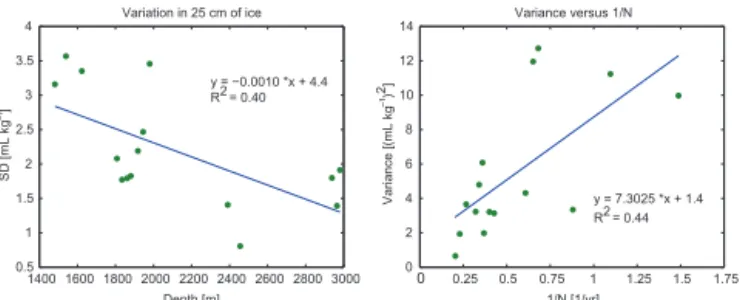
NGRIP ice), which is higher than the calculated analytical er-ror of 1.3 mL kg−1. This is expected due to natural variations of TAC in the ice along the 25 cm of ice core used for the reproducibility measurements (see also Sect. 3 below) and variations in the number and size of the air bubbles opened on the sides of the ice cube during cutting. In order to min-imize the latter effect, we cut all samples the same way, in pieces of∼40 g.
cov-Figure 2.The NGRIP TAC record of this study on the AICC2012
gas age scale (Veres et al., 2013), using two different methods. Blue: the melt–refreeze data; turquoise: the vacuum-melt TAC. The red line represents a spline with a 750-year cutoff period, according to
Enting (1987). At the bottom, theδ18Oicefor the NGRIP ice core
(NGRIP Project Members, 2004) is given.
1400 1600 1800 2000 2200 2400 2600 2800 3000 0.5
1 1.5 2 2.5 3 3.5
4 Variation in 25 cm of ice
Depth [m]
SD [mL kg ]
y = −0.0010 *x + 4.4
R2 = 0.40
0 0.25 0.5 0.75 1 1.25 1.5 1.75 0
2 4 6 8 10 12
14 Variance versus 1/N
1/N [1/yr]
Var
iance [(
mL kg )
2]
y = 7.3025 *x + 1.4
R2 = 0.44
–1
–1
Figure 3.Left: standard deviation of reproducibility measurements
in the TAC dependent on depth. Each point represents the mean over five adjacent samples. As expected, the variations get smaller with the smoothing due to thinner annual layers. Right: the variation of
the reproducibility measurements vs. 1/N, whereNis the number
of annual cycles in the sample.
ered in the 25 cm of the adjacent reproducibility samples. The measured variation should therefore decrease with 1/N,N
being the number of years contained in one sample, and the five samples in each 25 cm interval provide us with informa-tion on the analytical error according to
σmeasured2 =σ
2 ice
N +σ
2
analytical. (5)
IfN approaches infinity we get an independent estimate of
our analytical error. In Fig. 3 in the right panel we display the variation in the reproducibility samples vs. 1/Nwith the best
linear fit. We get ay intersect (corresponding toN= ∞) of
1.4 mL2kg−2. If the square root is taken, this independent es-timate leads to an analytical error of 1.2 mL kg−1, very close to the 1.3 mL kg−1we calculated in Sect. 2.1.1.
Most of our TAC data (years 2010–2012) were measured using the above described method, while data obtained be-tween 2002 and 2004, 287 samples in total, were measured with a slightly different procedure, as described in Flückiger et al. (2004). The main difference is that at that time the evac-uation step after loading the ice into the vessel lasted for 2 h
Table 1.List of abbreviations in the order in which they are first
used.
Abbreviation(s) Denotation
TAC Total air content (in literature also calledV) Vc,Pc,Tc Volume, pressure and temperature at close-off P0,T0 Standard pressure and temperature
m Mass of the ice sample n Mole number
V2 Volume of the sampling loop
V1,Vh,Vt Volumes in the apparatus, withV1=Vh+Vt and h for headspace, t for transition
T1,T2 The temperature in the abovementioned volumes V1andV2
ISI, sISI Integrated summer insolation, standardized ISI Vcr Non-thermal residual term of the pore volume TAC∗ −TAC−TAC
σ(TAC) Vcr∗ −Vcr−Vcr
σ(Vcr)
Vmol The volume of one mol at STP
instead of about 30 min, and the released air was expanded three times in sequence into a smaller, unchilled sampling loop for analysis. For those measurements the TAC was de-termined three times per sample and the analytical error of TAC was estimated as the standard deviation of the three measurements, leading to individual error bars for each data point with an average error of 2.86 mL kg−1.
2.1.2 Offset correction in the melt–refreeze data
The 2002–2004 and 2010–2012 data are slightly offset from each other, so a method to intercalibrate the two data sets was developed. Also, between the measurement periods of 2010, 2011 and 2012, minor changes in the instrument could lead to small offsets which have to be accounted for. Data pairs of corresponding sample depths in the NGRIP ice core from the different measuring periods were identified, the measur-ing period of 2012 was taken as a reference. Reference data points are compared with interpolated values of the other dataset. Only the data from 2010 could not be compared di-rectly to 2012 because they cover different sections of the ice core, and hence the 2010 data set was compared to the 2011 data. The mean of the offset values is displayed in Ta-ble 1 together with its standard error. The age differences to the closest points of the reference values are also shown in Table 2, with the interpolations providing better results if the data points are closer to each other, as expected from the natural variability of TAC in the ice. Based on this com-parison, the data from 2002 were shifted by 3.4 mL kg−1, those from 2004 by 6.1 mL kg−1 and those from 2011 by
−2 mL kg−1. The 2010 data are not significantly different
(1.2±1.4 mL kg−1) from 2012, so no correction was made.
0 5 10 15 20 25 30 35 40 45 Age [kyr BP]
75 80 85 90 95 100 105 110 115 120
TAC [mL kg ]
-8 -6 -4 -2 0 2 4 6
Difference [mL kg ]
NGRIP-GRIP comparison NGRIP melt-refreeze GRIP
NGRIP vacuum-melt
–1
–1
Figure 4.GRIP TAC data (Raynaud et al., 1997) in brown, vacuum-melt TAC data in yellow and vacuum-melt–refreeze TAC data in blue. All data on the synchronized ice age scale for GRIP and NGRIP are according to Seierstad et al. (2014). The black curve at the bottom represents the difference between GRIP and NGRIP TAC data in 2 kyr intervals.
3 The NGRIP TAC record
Our new NGRIP record contains 1688 TAC data points and is shown in Fig. 2 on the AICC2012 gas age scale (Veres et al., 2013), along withδ18Oice. The depth range is 133.81 to 3082.23 m, which corresponds to 294 to 119 555 years in gas age on the AICC2012 timescale.
3.1 Comparison with GRIP TAC
Raynaud et al. (1997) presented a lower-resolution Green-land TAC data set from the GRIP ice core. GRIP is located 316 km south-southeast of NGRIP, at an altitude of 3232 m, compared to 2919 m at NGRIP (Dahl-Jensen et al., 1997). Today there is essentially no temperature difference between NGRIP and GRIP as the altitude effect is compensated for by the higher latitude of the former. Therefore, and because insolation differences are insignificant between the two sites due to their geographic proximity, we do not expect any dif-ference either in pore volume Vc (Martinerie et al. (1992). Accordingly, assuming the temperature consistency did also not change in the past, the only factor influencing the TAC difference between the two sites is altitude (and possibly wind (Martinerie et al., 1994), which is ignored here). The GRIP data mainly cover the Holocene with measurements back to 40.6 ka BP. In Fig. 4 we show the TAC from Ray-naud et al. (1997), along with our two TAC records (melt– refreeze and vacuum-melt) in the time interval 0.2 to 45 ka BP on gas age. The GRIP and NGRIP data are given on a synchronized ice age scale for the Greenland records (Seier-stad et al., 2014). The data show good agreement; the GRIP
Table 2.Table with the offsets between the data from different
mea-suring periods. The second number in the intervals column is the reference period. Offset values are the median of all data points
compared. The given error is the standard error.n is the number
of points compared. Av. age offset denotes the average difference to the closer endpoint of the interpolation interval. The 2010 data could not be compared directly to 2012, so the offset values in the table are calculated from the other offsets.
Intervals Offset n Av. age
(yr) (mL kg−1) (offset yr)
2004 and 2012 −6.1±0.6 33 196
2002 and 2012 −3.4±2.1 24 348
2010 and 2011 3.16±0.9 37 47
2012 and 2011 −2.0±1.1 24 344
2010 and 2012 1.2±1.4 – –
TAC air content is on average slightly lower. To quantify the difference, each point from GRIP was compared with at most the two nearest neighbors of the NGRIP data in each time di-rection if they lay within 250 years of the GRIP data point. Up to 11.5 ka (Holocene) GRIP data were only compared to vacuum-melt data since no melt–refreeze data were avail-able. The Holocene GRIP TAC is about 1.7±0.3 mL kg−1
lower than NGRIP, and glacial GRIP in the interval 11.5 to 45 ka is 2.4±0.3 mL kg−1lower, where the error is the
stan-dard error of the mean. This is generally in line with the ex-pectations: a higher altitude at the deposition site should lead to lower TAC. Our results are different by 1σ, which is
al-most a non-significant difference, but they leave room for small relative altitude changes from the Last Glacial Max-imum (LGM) to the Holocene between the two sites, al-though other studies (e.g. NGRIP Project Members, 2004) state that the relative altitude changes are believed to be small. Assuming a mean annual temperature of −46◦C
(−31.5◦C) for stadial (Holocene) conditions (Kindler et al.,
2014) at NGRIP and using the barometric formula leads to a pressure–elevation gradient ofδP /δZ=10.5 hPa/100 m
4 Discussion
4.1 Low-frequency variations in TAC
TAC in Antarctica is known to show an anti-correlation with the integrated local summer insolation (ISI) as shown by Raynaud et al. (2007) for approximately the last 400 000 years in the EPICA Dome C record. We define ISI as
ISI=
365
X
i=1
wi·θ(wi−w0), (6)
where wi is the daily insolation in W m−2, θ is the
Heav-iside step function and w0 denotes a threshold insolation. This threshold had been defined by tuning the correlation be-tween ISI and TAC. A similar dependency emerges for our Greenland ice core when calculating a local summer inso-lation for the NGRIP drill site. A maximum correinso-lation be-tween TAC and ISI is found forw0=390 W m−2, compared
to 380 W m−2used by Raynaud et al. (2007) for the Antarc-tic EPICA Dome C (EDC) ice core. The correlation differ-ence between 380 and 390 W m−2 is, however, small, and the threshold does not alter the shape of the ISI much.
Martinerie et al. (1992) found an empirical relationship be-tween the pore volumeVcat bubble close-off and the temper-ature for recent equilibrium densification conditions with
Vc=0.76·
mL
K·kg
·Ts−57·
mL
kg
, (7)
whereTs is the snow temperature in Kelvin, here assumed to be the same as the temperature at bubble close-off depth,
Tc, when the firn column is in thermal equilibrium. Like in Raynaud et al. (2007), we defined the non-thermal residual termVcras
Vcr=TAC·Tc
Pc· P0
T0−Vc(Ts), (8)
whereTc andPcare the temperature and pressure at bubble close-off depth. For the temperature at bubble close-off we used values by Kindler et al. (2014) which are derived from a heat conduction model and surface temperature variations us-ing theδ15N thermo-diffusion technique (Severinghaus and
Brook, 1999; Lang et al., 1999; Kindler et al., 2014), provid-ing data from 10 to 120 ka. For the pressure at bubble close-off, we use a constant value of 699 hPa.T0 andP0 are the
standard temperature (273 K) and standard atmospheric pres-sure (1013 hPa), respectively. Analogous to Raynaud et al. (2007) and Lipenkov et al. (2011), we define a standardized version of TAC andVcr:
TAC∗= −TAC−TAC
σ(TAC) (9)
and
Vcr∗= −Vcr−Vcr
σ(Vcr) . (10)
10 20 30 40 50 60 70 80 90 100 110 120
Age [kyr BP]
-2 0 2
Standarized data
Figure 5.Red: the standardized 75.1◦N integrated summer
insola-tion sISI on days with more than 390 W m−2, splined with a 3 kyr
cutoff period. Blue: a standardized spline with a 750-year cutoff of
the TAC∗ record. Green: analogous to Raynaud et al. (2007) the
TAC∗data after correcting for the temperature effect on pore
vol-umeVcr(Martinerie et al., 1992). Note that the ice core data are
given on the glaciological AICC2012 ice age scale (as solar insola-tion acts on the snow matrix and therefore on changes in TAC on the ice age scale), while ISI is on the absolute astronomical age scale.
Splines with a 750-year cutoff period (Enting, 1987) through TAC∗andV∗
cr are shown together with the standardized ISI (sISI), splined with a 3 kyr cutoff period, in Fig. 5.
Ther2 between TAC∗ andVcr∗ for the spline is 0.95, so
the temperature effect on firnification processes quantified according to Martinerie et al. (1992) is responsible for only 5 % of the TAC variance, in accordance with Raynaud et al. (2007). These authors derived anr2 of 0.86 and estimated
the temperature-induced TAC variations to 10% of the total signal. The strong covariance of TAC∗and local insolation for both Greenland and Antarctic ice cores provide indepen-dent evidence of an ISI effect on pore volume as the temporal evolution of ISI in both hemispheres differs significantly. As can be seen in Fig. 5, the shape of the sISI is highly covari-ant with the low-frequency variations of TAC∗andV∗
cr, while higher-frequency variations seem to correlate with tempera-ture on the ice sheet (see Fig. 2). Note that during the glacial, temperature changes in Greenland are dominated by fast DO events, and a spline through the data filters out some of the variations.
Investigations on the higher frequency variations and TAC relation to climate changes during DO events are dis-cussed in Sect. 4.3.2. In Table 3 the correlations between the sISI, Vcr∗, Tc and TAC∗ are shown. For the best lin-ear fit we estimate a sensitivity of TAC on the local inte-grated summer insolation’s energy input above 390 W m−2 of−5.7×10⁻⁹mL kg−1J−1with anr2of 0.3.
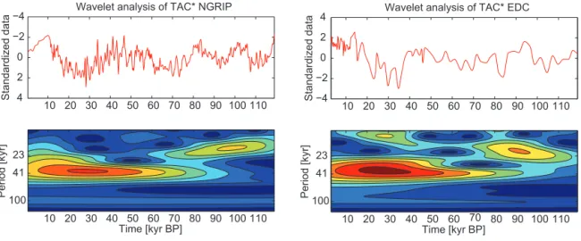
10 20 30 40 50 60 70 80 90 100 110
−4 −2
0
2
4
Wavelet analysis of TAC* NGRIP
Standardized data
Time [kyr BP]
Period [kyr]
10 20 30 40 50 60 70 80 90 100 110 23
41
100
10 20 30 40 50 60 70 80 90 100 110
−4 −2
0 2
4 Wavelet analysis of TAC* EDC
Standardized data
Time [kyr BP]
Period [kyr]
10 20 30 40 50 60 70 80 90 100 110 23
41
100
Figure 6.Left: the TAC∗data in red, resampled at an age step of 0.2 kyr and wavelet analysis of this spline. Right: EDC TAC∗data (Raynaud
et al., 2007), resampled at 0.2 kyr and its wavelet analysis in the same time window.
are also related to ice sheet changes. Models for Greenland ice sheet coverage and surface height in the Eemian show little difference to the present. Using on ice sheet modeling, Born and Nisancioglu (2012) estimate at NGRIP a maximum lowering of 200 m in the LGM compared to the Holocene. Using the same calculations as in Sect. 3.1, this would ac-count for a TAC change of 2.4 mL kg−1, while the observed TAC changes at the very end of the TAC record are in the order of 10 mL kg−1.
Note that the correlation breakdown between TAC and ISI before 109 ka mainly results from only two data points (see Fig. 2), at 118.8 and 119.4 ka with very low TAC, and the robustness of the TAC/ISI decoupling can therefore be ques-tioned. If we exclude these two points and correlate the sISI with the TAC∗from the top only until 109 ka,r2increases to 0.45, while the absolute changes in TAC are still larger than expected from altitude changes in models.
It has to be taken into account that the timescale of ISI is absolute, while the AICC2012 age scale used in this study is fundamentally based on an ice-flow model and in partic-ular shows younger ages for the lowest part of the ice core, compared to other timescales (Veres et al., 2013), with an uncertainty of around 5000 years in the lowest part of the ice core. Accordingly, if the older part of the TAC record were shifted to somewhat older ages, the correlation would increase. This would imply that the lowest part of the NGRIP ice core contains not the end of the Eemian but its maxi-mum. The comparison of the NGRIP and NEEM ice and gas records over the Eemian compiled by Landais et al. (2016) shows that such a stretching of the NGRIP record’s lowest part would then lead to consistency problems between the NEEM gas records and their Antarctic counterparts, which were used as a template to date the bottommost ice at NEEM. Accordingly, a simple shift of the AICC2012 age scale used for the NGRIP ice core in Fig. 5 seems incompatible with the
Table 3.Table with the squared correlation coefficients between
data and calculated parameters TAC∗, sISI, V∗
crandTc.
TAC∗ sISI V∗
cr Tc
TAC∗ – 0.31 0.95 0.26
sISI 0.31 – 0.24 0.01
NEEM ice core. We therefore refrain from providing a new orbitally tuned age scale for the oldest part of the NGRIP record. Instead, other factors than the age scale appear to be responsible for the deviation of TAC from ISI at that time.
4.2 Spectral analysis
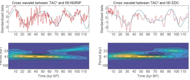
Following Raynaud et al. (2007), we performed a wavelet analysis on the TAC data (Fig. 6). Between 20 and 70 ka the obliquity effect on TAC is dominant, while for 80–110 ka the precession cycle dominates. This is in agreement with the findings for EDC, displayed in the right panel of Fig. 6. Since both Antarctic EDC and Greenland NGRIP TAC show the same pattern of either obliquity or precession dominance, we performed a cross-wavelet analysis between the TAC and the respective local ISIs. This analysis allows us to find common spectral signals in the time series (see, e.g., Grinsted et al., 2004; Fig. 7).
Figure 7.Left: the TAC∗data, resampled at 0.2 kyr in red; sISI with a threshold of 390 W m−2in blue, splined with a 3 kyr cutoff period
and cross-wavelet analysis thereof. Both records show coherence in the obliquity and precession bands. Right: EDC TAC∗(Raynaud et al.,
2007) resampled at 0.2 kyr, sISI (75.1◦S) with a threshold of 380 W m−2and cross-wavelet analysis of the EDC and sISI.
1860 1870 1880 1890 1900 1910 1920 90
95 100 105 110
TAC [mL kg ]
0 2 4 6 8
Dust [mg kg ]
-46 -44 -42 -40 -38
d
18
350 400 450 500 550
CH
4
[ppbv]
2100 2110 2120 2130 2140 2150 Depth [m]
2510 2520 2530 2540 2550 2560 0 0.2 0.4 0.6 0.8
Ca
[mg kg ]
2+
3 3 3
4 4 4
9 9 9
10 10
10
19 19 19
–1
–1
–1
Figure 8.Zoom into DO events 3, 4, 9, 10 and 19 on depth scale. Blue: the TAC, including a spline with a 120 m cutoff (thick red
line). Black: the dust; grey: the Ca2+concentration (Ruth, 2007).
Green: CH4; red: theδ18Oice. Grey lines indicate the beginning
of the DO events in CH4. More on the timing of TAC changes in
Sect. 4.3.2 and in Figs. 9 and 10
4.3 Higher-frequency TAC variations and DO events 4.3.1 Relation to Ca2+/dust
Based on recent studies (Freitag et al., 2013), small-scale firn density is known to correlate with Ca2+ tions in the ice representative of mineral dust concentra-tion. Accordingly, a firnification effect of dust on pore vol-ume has been proposed (Hörhold et al., 2012), which should be most pronounced for stadial–interstadial variations when dust concentrations in Greenland changed by a factor of about 15 (Fischer et al., 2007). As the TAC is a result of the competing process of densification and water vapor trans-port/recrystallization, an influence of Ca2+concentration on
TAC could also be hypothesized. In Fig. 8 the NGRIP TAC, dust and Ca2+ (Ruth, 2007), CH
4, andδ18Oice records are shown on the depth scale for selected DO events. No sim-ple relation from TAC with the dust concentration can be ob-served. Moreover, the TAC variations on their depth scale are not in phase with dust and Ca2+concentrations, as would be expected from a direct firnification effect of dust concentra-tions in the ice matrix on pore volume at bubble close-off. In-stead, the high-frequency variations in TAC seem to change in parallel with CH4and therefore on the gas age scale, sug-gesting a direct influence of temperature on the number of moles of air enclosed in the pore volume during bubble close-off. We will discuss this anti-correlation in the next section.
4.3.2 Relation to climate changes during DO events The TAC data (Fig. 2) not only show low-frequency vari-ations as discussed in Sect. 4.1 but reveal a strong high-frequency signal. Making use of the unprecedented resolu-tion of our record, we investigate the high-frequency vari-ations and take a closer look at what happens to the TAC during DO events.
The temperature effect (Eq. 7) on the pore volume created during steady-state densification would lead to a very small increase in pore volume with rising temperatures. Using the ideal gas law, we obtain
TAC=Vmol·n=Vmol·Pc·Vc(Ts) R·Ts
=Pc·Vmol
R ·(0.76−
57 K
Ts ), (11)
whereVmolis the volume of one mol at STP,Vc(T) the pore
Figure 9.The significant minima in the TAC spline with 750-year
cutoff from 10 to 120 ka BP. The measured TAC on AICC2012 gas age scale is blue; the spline is green. Minima marked by ruby lines are considered significant by the algorithm described in the text, while significant minima without a close-by DO event are indicated
by grey dashed lines. Red: theδ18Oiceon the AICC2012 ice age
scale.
enclosed in the bubbles. Therefore, a slight increase in TAC with increasing temperature is expected from the pore vol-ume effect. However, the formula for pore volvol-ume changes, derived in Martinerie et al. (1992) based on steady-state Holocene conditions, is most likely not applicable during DO events where a transient change in densification occurs. It is reasonable to assume that the pore volume in the firn does not follow this temperature relationship (Eq. 7) directly at the onsets of DO events. If we assume that the pore volume remains constant during the very first stage of a DO event, the first-order effect of slowly increasing temperatures in the firn would lead to a decrease in TAC, as supported by our data (Fig. 2). To test objectively whether there is a coherent pattern of decreasing TAC at the onset DO events, we devel-oped a method to find significant TAC decreases. To remove noise in the TAC raw data, 1000 Monte Carlo splines (vary-ing the data points randomly within their error before calcu-lating each spline fit) with a cutoff period of 750 years were calculated on the AICC2012 gas age scale, and the mean of the 1000 splines was taken as our best-guess representation of true TAC variations (Monte Carlo average, MCA). This MCA spline is then searched for maxima and minima. A detected minimum is considered significant if the difference between the last maximum and the minimum is larger than 1.5 times the added standard deviation of the spline at both points. The result is shown in Fig. 9. With these criteria and parameters, the routine finds 23 significant minima, of which 17 are related to a DO event inδ18Oice. The significant
min-ima unassociated with a DO event occur at the onset of the Younger Dryas, two in the LGM and one during DO event 25. There is another one before DO event 24, which is due to a wiggle in the spline fit, leading to two significant minima in the descent preceding DO event 24 (see Fig. 9). Using the abovementioned parameters, the routine fails to find signif-icant minima related to DO events 8, 9, 16–18, 20, 22, 23 and 25, although for many of these cases a decline in TAC exists, which, however, did not satisfy our significance cri-terion. For DO events 9, 18 (and the event p18, in Fig. 9 regarded as a precursor event of DO event 18), 20, 23 and 25, this is due to the threshold of 1.5σbeing too high, while
16–17 follow each other very closely so the TAC response signal is not visible. For DO event 22 the detected minimum is more than 1000 years before theδ18Oicemaximum, so we considered this not to be related to the warming. DO event 22 has a small amplitude inδ18Oice compared to the back-ground and the other DOs; thus, only a small TAC response is expected.
Apparently, TAC shows an anti-correlation not only to ISI but also to rapid DO warmings. Again a comparison to the O2/N2ratios is of interest, since Suwa and Bender (2008) found not only a correlation of O2/N2to insolation but also a correlation of O2/N2ratios with DO warmings. We specu-late that both proxies are influenced by the same not yet fully understood firnification processes. The phasing of the TAC compared to the δ18Oice is also of interest. In Table 4 the timing of the TAC minima on the AICC2012 gas age scale and the maxima in the rises of δ18Oice on the AICC2012 ice age scale are shown. On average, the TAC minimum is synchronous with theδ18Oice maximum within the error (12±290 years) on the AICC2012 age scale. However, as
stated by Baumgartner et al. (2014), the AICC2012 gas age scale suffers from inconsistency with the AICC2012 ice age scale for several DO events as gas and ice have been synchro-nized between different ice cores to some extent indepen-dently. This leads to a dephasing of CH4andδ18Oicerecords in some cores on the AICC2012 age scale, which is absent in the original age scales, where gas age scale has been deter-mined by adding the gas-age–ice-age difference to the ice age scale. For this reason Kindler et al. (2014) published a new gas age scale for NGRIP, based on the ss09sea06bm (NGRIP Project Members, 2004) ice age scale, defined from 10 to 120 ka. Being aware of this inconsistency, we also derived the correspondingδ18Oicemaxima on ss09sea06bm ice age and the TAC spline minima on the gas age scale by Kindler et al. (2014). On those age scales theδ18Oicemaximum is reached on average 111±232 years earlier than the minimum in TAC
and only two DO events show the TAC minimum earlier than theδ18Oicemaximum. Neglecting DO 13, theδ18Oice
maxi-mum leads TAC by 162±108 years (37±217 years on the
-800 -600 -400 -200 0 200 Age [yrs]
-6 -4 -2 0 2 4 6
Relative temp [K]
-3 -2 -1 0 1 2 3
Relative TAC [mL kg ]
-1000 -800 -600 -400 -200 0 200 400
Age [yrs] -60
-40 -20 0 20 40
Relative CH
4
[ppbv]
-2 -1 0 1 2 3
Relative TAC [mL kg ]
-0.04 0 0.04 0.08
d
15
–1
–1
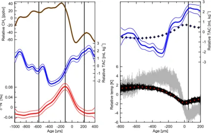
Figure 10.Stacked data over the onsets of all DO events except DO events 2 and 25 (Table 4). Left: red – the stackedδ15N model data
(Kindler et al., 2014); blue – the TAC; brown – CH4. Full lines represent the spline; thin lines the 1σ error range. Note that the variability
in the stacked concentration only refers to the analytical error and not the variability between different DO events. Grey lines indicate the
start, the maximum and the end of theδ15N signal. All three are given on AICC2012 gas age scale. Right: running mean over the modeled
bubble close-off temperature (Kindler et al., 2014) in black; red squares indicate a 50-year mean. Grey: the modeled surface temperature. Blue crosses represent the calculated TAC values dependent on bubble close-off temperature only. The blue lines represent the measured TAC on ice age scale. Note that the amplitude of the TAC response differs for the left and right plot, since the stack was established on a different age scale and thus not over the same time windows and with different starting points. The grey line indicates the onset of the surface temperature warming.
-800 -600 -400 -200 0 200 Relative age [yrs]
-48 -46 -44 -42 -40 -38 -36 -34
Temperature (°C)
-6 -5 -4 -3 -2 -1 0 1 2 3 4
TAC anomaly (mL/kg)
?
Figure 11.Modeled behavior of TAC for an idealized DO event
with a 10◦C linear surface warming during 100 years after the
on-set of the event. At the bottom, in grey, the assumed surface tem-perature and in black the temtem-perature at bubble close-off depth. At the top, in turquoise, the TAC model output for steady-state firni-fication conditions (Eq. 11). Blue: the transient firnifirni-fication model (Schwander et al., 1997) TAC output for a constant bubble close-off time. Dashed lines indicate the range of measured TAC anomalies.
DO events. Moreover, when comparingδ18Oicein the ice
ma-trix and a direct temperature-related signal in TAC, the uncer-tainty in the ice-age–gas-age difference has to be taken into account. Therefore, in the following we compare the TAC behavior to other proxies only on the same age scales.
To figure out how the TAC reacts in general to DO event warmings, we calculated a stack of TAC variations during
DO events and compared it to other gas phase parameters. Since the TAC seems to react in the time window where CH4 also shows changes, we stacked the TAC around the CH4 onsets. For this we defined a criterion for the rise in CH4. The analytical error in the CH4data is 5.9 ppbv (Baumgart-ner et al., 2014). The start of the CH4 increase was defined by Baumgartner et al. (2014) in the middle between the first two data points during the onset of stadial–interstadial tran-sitions which did not agree within their 3σ uncertainty
any-more. We used the same definition and translated the depth values on the AICC2012 gas age scale. Additionally, we de-fined the onset for DO 3 and 22 by applying only a 2σ
crite-rion, since with 3σ, no onset could be defined. These criteria
give the onsets given in Table 4, except for DO 2 and 25, for which the onset could not be defined. The same stacking analysis was performed forδ15N (Kindler et al., 2014),
in-dicating temperature gradients across the firn column caused by rapid warming at the surface. The TAC (this study) and the δ15N time series from Kindler et al. (2014) were then
cut out in age windows+400 and−1000 years around the
Table 4. Timing of the DO events and related features. The time value inδ18Oice denotes the maximum of the rise inδ18Oice on the
AICC2012 ice age scale, determined visually. The time point in TAC is the time of the minimum, found with the method described in
Sect. 4.3.2. On average theδ18Oice rise is younger by−12±290 years with a median of−10 years on the AICC2012 age scale. The
corresponding values on the sso9sea06bm ice age scale and the gas age scale published by Kindler et al. (2014) are also shown in the second
block of the table. On average theδ18Oicerise is older by 111±233 years with a median of 140 years on these age scales. The third block
shows the timing of the onset in CH4used for the stacking in Fig. 10a on the AICC2012 gas age scale (Veres et al., 2013). In the forth block,
the onsets in bubble close-off temperatureTcodused for the stacking in Fig. 10b on the AICC2012 ice age scale are displayed.
DO δ18Oice TAC Diff. δ18Oice TAC Diff. CH4 Tcod (AICC2012 ice) (AICC2012 gas) (yr) ss09sea06bm (Kindler gas) (yr) (AICC2012 gas) (AICC2012 ice)
PB 11 570 11 580 −10 11 464 11 390 74 – –
BA 14 551 14 560 −9 14 534 14 439 95 14 904 15 780
2 23 251 23 600 −349 22 669 22 569 100 – 22 100
3 27 691 27 820 −129 27 364 27 264 100 28 117 29 060
4 28 751 28 790 −39 28 462 28 303 158 29 280 30 440
5 32 410 32 660 −250 32 217 32 064 153 33 062 33 740
6 33 630 33 810 −180 33 519 33 384 134 34 246 34 960
7 35 390 35 480 −90 35 335 35 199 136 35 918 36 880
8 – – – – – – 38 303 40 120
9 – – – – – – 40 273 41 120
10 41 391 41 220 171 41 728 41 560 168 41 521 42 580 11 43 270 43 140 130 43 657 43 459 198 43 445 44 560 12 46 789 46 610 179 47 355 47 215 140 46 851 47 960 13 49 210 50 020 −810 49 782 50 504 −722 49 341 50 120
14 54 151 53 880 271 55 056 54 745 311 54 294 55 200 15 55 651 55 440 211 56 516 56 314 202 55 837 56 740
16 – – – – – – 58 106 58 980
17 – – – – – – 59 086 –
18 – – – – – – 64 059 65 520
19 72 087 71 940 147 72 957 72 815 142 72 095 73 320
20 – – – – – – 75 860 76 820
21 84 130 83 570 560 85 421 84 925 496 84 101 84 780
22 – – – – – – 89 402 90 040
23 – – – – – – 101 844 102 320
24 105 747 105 760 −13 108 882 108 886 −4 106 065 10 660
25 – – – – – – – 113 240
Average −12±290 Average 111±233
Median −10 Median 140
were then stacked and for each of them – the CH4, the TAC, andδ15N data – a spline with a cutoff period of 200 years
was calculated. The result is displayed in the left panel of Fig. 10. Relative to CH4, the measured TAC decrease starts around 100 years earlier. Within the error,δ15N starts to
in-crease synchronously with TAC. This 100-year lag of CH4 to temperature is somewhat more than the 25–70±25 years
calculated for DO events in Marine Isotope Stage 3 in pre-vious studies (Huber et al., 2006) and clearly more than the 4.5+21
−24years for the Bølling–Allerød interstadial (BA) calcu-lated in Rosen et al. (2014). This difference may partly be attributed to the different methods used in the various pub-lications to detect the onset in the CH4 rise and/or may be specific to the BA warming. Note that the stacked TAC data show a two-step decrease that lasts for several hundred years. When theδ15N signal reaches its maximum, TAC is still
de-creasing; shortly before theδ15N stabilizes, the TAC slightly
rises and then drops in a second step to lower values than before the event.
The total amplitude of the TAC response in Fig. 10a is
−4.7±0.7 mL kg−1. Using Eq. (1) with all parameters but
the temperature fixed, we can calculate the expected physi-cal TAC response according to the ideal gas law (Fig. 10b). The temperature influencing the TAC is the bubble close-off temperature, as derived by Kindler et al. (2014) using a heat transport model with the surface temperature determined by
δ15N thermodiffusion thermometry. To get an average
be-havior of bubble close-off temperature, we also stacked this modeled firn temperature at bubble close-off for the DO events in windows of+200 to−800 years relative to the
on-set in close-off temperature (see Table 4). We then calculated the mean over 50-year intervals from +175 to −775 year
provided by Kindler et al. (2014) on a depth scale, trans-lated to the AICC2012 ice age scale. With a starting tem-perature and TAC of 227.15 K and 90 mL kg−1, respectively, we computed the expected TAC response (blue crosses in Fig. 10b). Also shown in Fig. 10b are the measured TAC val-ues on ice age scale for comparison with the modeled TAC and the temperature at the surface. The calculated amplitude of the direct temperature effect through the ideal gas law (number density of molecules per volume) at bubble close-off is 1.4 mL kg−1, which is only about a third of the mea-sured one. The amplitude difference indicates that other ef-fects than the temperature at bubble close-off influence TAC on short timescales and especially during the second step of the TAC decrease, where in situ gas temperature changes are already quite small.
One possibility of explaining the larger TAC amplitude than expected from the direct temperature effect could be co-occurring changes in surface pressure, for example related to synoptic pressure pattern changes related to DO events. To explain the full amplitude in DO event TAC changes, how-ever, a pressure decrease at the NGRIP site of around 17 hPa would be required during interstadial warmings, potentially related to a northward shift of North Atlantic storm tracks (Kageyama et al., 2009) connected to a drastic reduction of sea ice during DO events which would also lead to a lower-ing of synoptic pressure over Greenland (Zhang et al., 2014). However, compared to currently observed spatial gradients in mean annual sea level pressure over the North Atlantic, the size of this effect appears too large and, moreover, should oc-cur synchronously with the onset of the DO events and thus is unlikely to explain the TAC changes in later stages of the DO events. In contrast, a transient effect of changes in firni-fication, hence pore volume, during Greenland interstadials appears more likely to explain our observations. We suggest that such an effect can be induced by the rapidly increasing accumulation rate at the onset of the DO event. This leads to a higher load and thus enhanced deformation of the snow grains at depth at a time when the temperature in the firn col-umn is still cold. A simple transient firnification model ex-periment (Sect. 4.3.3) supports this hypothesis by reducing TAC by several milliliters per kilogram as in our observa-tions. In the following we attempt to quantify an upper limit of this transient firnification effect using a standard firnifica-tion model (Schwander et al., 1997).
4.3.3 Transient firnification model experiment
Empirical equations for estimating bubble close-off densities and bubble close-off depths have been derived for steady-state conditions (Martinerie et al., 1992, 1994). However, es-pecially at the beginning of a DO event the firn layer is far from being in a steady state condition. Fast artificial den-sification experiments of snow by applying high pressures resulted in very low TAC compared to natural firnification (B. Stauffer, personal communication, 2015). The reason for
low TAC in artificially densified ice is most likely that, due to the extremely high densification rate, there is not enough time to form spherical cavities, which are a result of min-imizing surface energy by slow mass redeposition through vapor diffusion. At the beginning of a DO event, accumula-tion increases in a step-like fashion, causing (less drastically but analogous to the artificial experiments) additional pres-sure in the bubble close-off zone by the increasing load of snow. We therefore expect a pore volume reduction and ex-pulsion of air from the firn, yielding to lower TAC compared to steady-state conditions.
We estimate the upper limit of this effect by assuming that for some 140 annual layers above the firn–ice transition in the firnification model, the time required to reach bubble close-off remains unchanged after a transition to a DO event. This assumption is based on the fact that the temperature at the depth of bubble close-off remains near the cold state during the first 140 years of a DO event (less than 20 % temper-ature response compared to the surface tempertemper-ature change; Fig. 10) and on the hypothesis that time is more important for finalizing the bubble close-off than the additional hydrostatic pressure.
We have used a standard dynamic firn densification model (Schwander et al., 1997) to calculate this upper limit for a typical DO event. In addition to computing the time and depth where the steady-state close-off density is reached (as in the normal usage of the model) the model provides the density that a firn layer reaches after a certain number of years. This number of years was set to the duration needed to reach close-off under interstadial conditions. Under the abovementioned assumption of an initially constant duration to reach close-off, this density reflects the true close-off den-sity and corresponding TAC better than values obtained for steady-state stadial conditions. Stadial temperature is set to
−46◦C and the ice accumulation rate to 0.05 m a−1. At the
beginning of the simulated DO event, we increase the tem-perature from−46 to−36◦C and the ice accumulation rate
from 0.05 to 0.1 m yr−1within 100 years, based on the model data by Kindler et al. (2014). The resulting TAC of the simu-lation is shown in Fig. 11. We interpret the resulting decrease in TAC as the upper limit scenario for the first 140-years of a DO event. The real effect might be smaller. Later, when the temperature at the firn–ice transition increases further, TAC will slowly approach the new equilibrium value. As there ex-ists no physical model describing this dynamic behavior of densification and bubble close-off to date, we cannot provide a more precise modeled evolution of TAC during a DO event, but the decrease in TAC as observed in the NGRIP ice core seems to be compatible with the simulation.
5 Conclusions
with previous studies in Antarctica (Raynaud et al., 2007; Lipenkov et al., 2011), we find the low-frequency variations to depend on local summer insolation and thus the orbital pa-rameters. Those effects act on the firn matrix controlling the pore volume during bubble close-off and, thus, operate on the ice age scale, (e.g. Raynaud et al., 2007; Bender, 2002), al-though the underlying processes are not yet understood. Ad-ditionally, in steady state, the pore volume is known to cor-relate with firn temperature (Martinerie et al., 1992), which is also an ice property leading to TAC changes. Our study shows that this temperature effect imprinted on pore volume during densification in steady state is small compared to the insolation effect operating at the surface and also small com-pared to a direct temperature effect on TAC imposed by the change in density of the gas during bubble enclosure that we clearly observe during DO events.
Comparison of δ15N, CH4 and TAC, all on the gas age scale, provides evidence that surface temperature warming, or an effect synchronous with surface warming, has a direct imprint on the TAC. The immediate decrease in TAC at an onset of a DO event could have two possible sources ac-cording to the ideal gas law: decreasing air pressure or less amount of substance per volume due to rising temperature. However, both effects appear to be too small to explain the measured TAC decline. Large changes in the height of the ice sheet are ruled out for such very short-term variations as the TAC change occurs immediately with the DO event warming, while the ice sheet response would be slow and delayed. However, the increasing accumulation rate during DO events leads to an increase in firn thickness of several tens of meters, which, through the additional weight on the firn column, leads to a temporarily enhanced densification. This could reduce TAC for several centuries after the on-set of the DO event. After 500–1000 years, the firn column reaches a new equilibrium with ambient temperature, accu-mulation and pore volume, and TAC reaches its steady-state value again.
With the TAC signal being influenced by effects on the ice age and gas age scale, this also limits the precision of de-riving orbital timescales from TAC for Greenland ice cores, which experience the rapid millennial scale DO variability which is absent for Antarctic ice cores.
6 Data availability
The NGRIP TAC data are available at https://www.ncdc. noaa.gov/paleo/study/20569.
Acknowledgements. Continuing support by the Swiss National Science Foundation for ice core research at the University of Bern is gratefully acknowledged. NGRIP is coordinated by the Depart-ment of Geophysics at the Niels Bohr Institute for Astronomy, Physics and Geophysics, University of Copenhagen. It is supported by Funding Agencies in Denmark (SHF), Belgium (FNRS-CFB),
France (IPEV and INSU/CNRS), Germany (AWI), Iceland (Ran-nIs), Japan (MEXT), Sweden (SPRS), Switzerland (SNF) and the United States of America (NSF, Office of Polar Programs). We thank J. Freitag for fruitful discussion on firnification and bubble enclosure processes.
Edited by: C. Barbante
Reviewed by: two anonymous referees
References
Baumgartner, M.: Bipolar reconstructions of atmospheric methane and nitrous oxide during the las glacial-interglaccial cycle, PhD thesis, Physics Institute, University of Bern, Switzerland, 194 pp., 2013.
Baumgartner, M., Schilt, A., Eicher, O., Schmitt, J., Schwander, J., Spahni, R., Fischer, H., and Stocker, T. F.: High-resolution inter-polar difference of atmospheric methane around the Last Glacial Maximum, Biogeosciences, 9, 3961–3977, doi:10.5194/bg-9-3961-2012, 2012.
Baumgartner, M., Kindler, P., Eicher, O., Floch, G., Schilt, A., Schwander, J., Spahni, R., Capron, E., Chappellaz, J.,
Leuen-berger, M., Fischer, H., and Stocker, T. F.: NGRIP CH4
con-centration from 120 to 10 kyr before present and its relation to
aδ15N temperature reconstruction from the same ice core, Clim.
Past, 10, 903–920, doi:10.5194/cp-10-903-2014, 2014.
Bender, M. L.: Orbital tuning chronology for the Vostok climate record supported by trapped gas composition, Earth Planet. Sc. Lett., 204, 275–289, 2002.
Born, A. and Nisancioglu, K. H.: Melting of Northern Greenland during the last interglaciation, The Cryosphere, 6, 1239–1250, doi:10.5194/tc-6-1239-2012, 2012.
Dahl-Jensen, D., Gundestrup, N., Keller, K., Johnsen, S., Gogineni, S., Allen, C., Chuah, C., Miller, H., Kipfstuhl, S., and Wassing-ton, E.: A search in north Greenland for a new ice-core drill site, J. Glaciol., 43, 300–306, 1997.
Enting, I. G.: On the Use of Smoothing Splines to Filter CO2Data,
J. Geophys. Res.-Atmos., 92, 10977–10984, 1987.
Fischer, H., Siggaard-Andersen, M.-L., Ruth, U., Röthlisberger, R., and Wolff, E.: Glacial/interglacial changes in mineral dust and sea-salt records in polar ice cores: Sources, transport, and depo-sition, Rev. Geophys., 45, rG1002, doi:10.1029/2005RG000192, 2007.
Flückiger, J., Blunier, T., Stauffer, B., Chappellaz, J., Spahni, R., Kawamura, K., Schwander, J., Stocker, T., and Dahl-Jensen,
D.: N2O and CH4 variations during the last glacial epoch:
Insight into global processes, Global Biogeochem. Cy., 18, doi:10.1029/2003GB002122, 2004.
Freitag, J., Kipfstuhl, S., Laepple, T., and Wilhelms, F.: Impurity-controlled densification: a new model for stratified polar firn, J. Glaciol., 59, 1163–1169, doi:10.3189/2013JoG13J042, 2013. Grinsted, A., Moore, J. C., and Jevrejeva, S.: Application of the
cross wavelet transform and wavelet coherence to geophys-ical time series, Nonlin. Processes Geophys., 11, 561–566, doi:10.5194/npg-11-561-2004, 2004.
Iso-tope Stage 3 and its relation to CH4, Earth Planet. Sc. Lett., 243,
504–519, 2006.
Hutterli, M., Schneebeli, M., Freitag, J., Kipfstuhl, J., and Röthlis-berger, R.: Impact of local insolation on snow metamorphism and ice core records, Low Temperature Science, 68, 223–232, 2009. Hörhold, M., Laepple, T., Freitag, J., Bigler, M., Fischer, H.,
and Kipfstuhl, S.: On the impact of impurities on the densi-fication of polar firn, Earth Planet. Sc. Lett., 325–326, 93–99, doi:10.1016/j.epsl.2011.12.022, 2012.
Kageyama, M., Mignot, J., Swingedouw, D., Marzin, C., Alkama, R., and Marti, O.: Glacial climate sensitivity to different states of the Atlantic Meridional Overturning Circulation: results from the IPSL model, Clim. Past, 5, 551–570, doi:10.5194/cp-5-551-2009, 2009.
Kindler, P., Guillevic, M., Baumgartner, M., Schwander, J., Landais, A., and Leuenberger, M.: Temperature reconstruction from 10 to 120 kyr b2k from the NGRIP ice core, Clim. Past, 10, 887–902, doi:10.5194/cp-10-887-2014, 2014.
Krinner, G., Raynaud, D., Doutriaux, C., and Dang, H.: Simulations of the Last Glacial Maximum ice sheet surface climate: Implica-tions for the interpretation of ice core air content, J. Geophys. Res.-Atmos., 105, 2059–2070, 2000.
Landais, A., Masson-Delmotte, V., Capron, E., Langebroek, P. M., Bakker, P., Stone, E. J., Merz, N., Raible, C. C., Fischer, H., Orsi, A., Prié, F., Vinther, B., and Dahl-Jensen, D.: How warm was Greenland during the last interglacial period?, Clim. Past Dis-cuss., doi:10.5194/cp-2016-28, in review, 2016.
Lang, C., Leuenberger, M., Schwander, J., and Johnsen, S.: 16◦C
Rapid Temperature Variation in Central Greenland 70,000 Years Ago, Science, 286, 934–937, doi:10.1126/science.286.5441.934, 1999.
Lipenkov, V., Raynaud, D., Loutre, M., and Duval, P.: On the
poten-tial of coupling air content and O2/N2from trapped air for
es-tablishing an ice core chronology tuned on local insolation, Qua-ternary Sci. Rev., 30, 3280–3289, 2011.
Lorius, C., Raynaud, D., and Dolle, L.: Densité de la glace et Étude des gaz en profondeur dans un glacier antarctique, Tellus, 20, 449–460, 1968.
Martinerie, P., Raynaud, D., Etheridge, D. M., Barnola, J. M., and Mazaudier, D.: Physical and climatic parameters which influence the air content in polar ice, Earth Planet. Sc. Lett., 112, 1–13, 1992.
Martinerie, P., Lipenkov, V. Y., Raynaud, D., Chappellaz, J., Barkov, N. I., and Lorius, C.: Air content paleo record in the Vostok ice core (Antarctica): A mixed record of climatic and glaciological parameters, J. Geophys. Res., 99, 10565–10576, 1994.
NEEM community members: Eemian interglacial reconstructed from a Greenland folded ice core, Nature, 493, 489–494, doi:10.1038/nature11789, 2013.
NGRIP Project Members: High-resolution record of Northern Hemisphere climate extending into the last interglacial period, Nature, 431, 147–151, doi:10.1038/nature02805, 2004. Parrenin, F., Barnola, J.-M., Beer, J., Blunier, T., Castellano, E.,
Chappellaz, J., Dreyfus, G., Fischer, H., Fujita, S., Jouzel, J., Kawamura, K., Lemieux-Dudon, B., Loulergue, L., Masson-Delmotte, V., Narcisi, B., Petit, J.-R., Raisbeck, G., Raynaud, D., Ruth, U., Schwander, J., Severi, M., Spahni, R., Steffensen, J. P., Svensson, A., Udisti, R., Waelbroeck, C., and Wolff, E.: The
EDC3 chronology for the EPICA Dome C ice core, Clim. Past, 3, 485–497, doi:10.5194/cp-3-485-2007, 2007.
Raynaud, D. and Lebel, B.: Total gas content and surface elevation of polar ice sheets, Nature, 281, 289–291, 1979.
Raynaud, D. and Lorius, C.: Climatic implications of Total Gas Content in Ice at Camp Century, Nature, 243, 283–284, 1973. Raynaud, D., Chappellaz, J., Ritz, C., and Martinerie, P.: Air content
along the Greenland Ice Core Project core: A record of surface climatic parameters and elevation in Central Greenland, J. Geo-phys. Res., 102, 26607–26613, 1997.
Raynaud, D., Lipenkov, V., Lemieux-Dudon, B., Duval, P., Loutre, M.-F., and Lhomme, N.: The local insolation signature of air content in Antarctic ice. A new step toward an absolute dating of ice records, Earth Planet. Sc. Lett., 261, 337–349, doi:10.1016/j.epsl.2007.06.025, 2007.
Rosen, J. L., Brook, E. J., Severinghaus, J. P., Blunier, T., Mitchell, L. E., Lee, J. E., Edwards, J. S., and Gkinis, V.: An ice core record of near-synchronous global climate changes at the Bolling tran-sition, Nat. Geosci., 7, 459–463, doi:10.1038/ngeo2147, 2014. Ruth, U.: Dust concentration in the NGRIP ice core,
doi:10.1594/PANGAEA.587836, 2007.
Schilt, A., Baumgartner, M., Schwander, J., Buiron, D., Capron, E., Chappellaz, J., Loulergue, L., Schüpbach, S., Spahni, R., Fischer, H., and Stocker, T. F.: Atmospheric nitrous oxide during the last 140,000 years, Earth Planet. Sc. Lett., 300, 33–43, 2010. Schilt, A., Baumgartner, M., Eicher, O., Chappellaz, J., Schwander,
J., Fischer, H., and Stocker, T.: The response of atmospheric ni-trous oxide to climate variations during the last glacial period, Geophys. Res. Lett., 40, 1888–1893, doi:10.1002/grl.50380, 2013.
Schmitt, J., Schneider, R., and Fischer, H.: A sublimation technique
for high-precision measurements ofδ13CO2and mixing ratios of
CO2and N2O from air trapped in ice cores, Atmos. Meas. Tech.,
4, 1445–1461, doi:10.5194/amt-4-1445-2011, 2011.
Schmitt, J., Seth, B., Bock, M., and Fischer, H.: Online technique
for isotope and mixing ratios of CH4, N2O, Xe and mixing ratios
of organic trace gases on a single ice core sample, Atmos. Meas. Tech., 7, 2645–2665, doi:10.5194/amt-7-2645-2014, 2014. Schwander, J., Sowers, T., Barnola, J. M., Blunier, T., Malaizé, B.,
and Fuchs, A.: Age scale of the air in the Summit ice: Impli-cation for glacial-interglacial temperature change, J. Geophys. Res., 102, 19483–19494, 1997.
Seierstad, I. K., Abbott, P. M., Bigler, M., Blunier, T., Bourne, A. J., Brook, E., Buchardt, S. L., Buizert, C., Clausen, H. B., Cook, E., Dahl-Jensen, D., Davies, S. M., Guillevic, M., Johnsen, S. J., Pedersen, D. S., Popp, T. J., Rasmussen, S. O., Severing-haus, J. P., Svensson, A., and Vinther, B. M.: Consistently dated records from the Greenland GRIP, GISP2 and NGRIP ice cores
for the past 104 ka reveal regional millennial-scale delta18O
gradients with possible Heinrich event imprint, Quaternary Sci. Rev., 106, 29–46, doi:10.1016/j.quascirev.2014.10.032, 2014. Severinghaus, J. P. and Brook, E. J.: Abrupt Climate Change at the
End of the Last Glacial Period Inferred from Trapped Air in Polar Ice, Science, 286, 930–934, doi:10.1126/science.286.5441.930, 1999.
Suwa, M. and Bender, M. L.: O2/N2 ratios of occluded air in
Veres, D., Bazin, L., Landais, A., Toyé Mahamadou Kele, H., Lemieux-Dudon, B., Parrenin, F., Martinerie, P., Blayo, E., Blu-nier, T., Capron, E., Chappellaz, J., Rasmussen, S. O., Severi, M., Svensson, A., Vinther, B., and Wolff, E. W.: The Antarctic ice core chronology (AICC2012): an optimized multi-parameter and multi-site dating approach for the last 120 thousand years, Clim. Past, 9, 1733–1748, doi:10.5194/cp-9-1733-2013, 2013.