FINITE VOLUME METHODS AND ADAPTIVE REFINEMENT FOR GLOBAL TSUNAMI PROPAGATION AND LOCAL INUNDATION.
David L. George and Randall J. LeVeque Department of Applied Mathematics
University of Washington
Seattle, WA 98195 U.S.A.
ABSTRACT
The shallow water equations are a commonly accepted approximation governing tsunami propagation. Numerically capturing certain features of local tsunami inundation requires solving these equations in their physically relevant conservative form, as integral con-servation laws for depth and momentum. This form of the equations presents challenges when trying to numerically model global tsunami propagation, so often the best numerical methods for the local inundation regime are not suitable for the global propagation regime. The different regimes of tsunami flow belong to different spatial scales as well, and re-quire correspondingly different grid resolutions. The long wavelength of deep ocean tsunamis requires a large global scale computing domain, yet near the shore the propa-gating energy is compressed and focused by bathymetry in unpredictable ways. This can lead to large variations in energy and run-up even over small localized regions.
We have developed a finite volume method to deal with the diverse flow regimes of tsunamis. These methods are well suited for the inundation regime—they are robust in the presence of bores and steep gradients, or drying regions, and can capture the inundating shoreline and run-up features. Additionally, these methods are well-balanced, meaning that they can appropriately model global propagation.
INTRODUCTION
We will describe a type of finite volume numerical method that is useful for solving a class of hyperbolic equations, specifically the nonlinear shallow water equations. These equa-tions are one of the commonly accepted approximaequa-tions governing tsunami propagation and inundation. They can present various difficulties for numerical methods depending on the flow regimes of the solution—which can vary greatly. For instance, the shallow wa-ter equations can often accurately describe global propagation of tsunami waves as well as general features of inundating waves at the shoreline or flooding onto dry land. These equations even admit solutions with propagating bores or discontinuities that approximate breaking waves, which may exist in the runup regions depending on local bathymetry. Although the validity of the shallow water approximation becomes more tenuous in the inundation and flooding regimes, these equations still perform surprisingly well at de-scribing basic features of these flows, and are often the most efficient and least expensive practical model [11, 12].
Many methods have been developed for the shallow water equations; however, nu-merical methods differ in their utility for different flow regimes—often a method that works well for one regime may fail to be useful for other regimes. Our goal has been to develop a method that is robust and accurate for solving these equations in any of the diverse regimes.
THE SHALLOW WATER EQUATIONS
The shallow water equations can be derived in a number of ways and in a variety of forms, all of which rely on the basic assumption that the flow is vertically hydrostatic, or equivalently, that the vertical acceleration of water particles is negligible. The validity of this assumption can be demonstrated for flows with long wavelengths compared to depth. It may be a reasonable approximation for other flows as well, at least for the depth averaged horizontal velocities. Once this approximation is accepted, the most physically relevant and generally valid form of the equations is as an integral conservation law for mass and momentum, which in one dimension is
d dt
Rx2
x1 h dx+ (hu)
xr xl =0
d dt
Rx2
x1 hu dx+ 1 2gh
2+hu2xr
xl =− Rx2
x1 ghbxdx,
(1)
where h is the water depth, u is the horizontal velocity, g is the gravitational constant and bis the bottom surface elevation. The integral conservation law (1) is often used to deduce a set of PDEs for mass and momentum
h hu t + hu 1
2gh2+hu2
x =
0
−ghbx
where the subscripts imply differentiation. This set of PDEs can be manipulated further to yield the most common form of the shallow water equations
ηt+u(η−b)x=0
ut+u(u)x+gηx=0,
(3)
where η is the elevation of the water surface, η =h+b. The system (3) is the most
commonly used form for modeling tsunamis since it is the least problematic for global propagation, however, it is not always valid in the near shore region as will be described below.
HYPERBOLIC SYSTEMS OF CONSERVATION LAWS
The system (2) belongs to a broader class of conservation laws of the form
d dt
Rx2
x1 q(x,t)dx+f(q(x2,t))−f(q(x1,t)) =
Rx2
x1 ψ(q,x)dx, ∀(x1,x2), (4)
whereq∈lRmis a vector of conserved quantities, f(q)∈lRmis the flux of these quantities, andψ is a source term. If the solutionq(x,t)is differentiable, then (4) can be manipulated
into the form
Rx2
x1 [qt(x,t) +f(q(x,t))x−ψ(q,t)]dx=0, ∀(x1,x2), (5)
which implies the PDEs
qt(x,t) +f(q(x,t))x=ψ(q,t). (6)
Ifψ is nonzero, (4) is sometimes referred to as abalance lawdue to the contribution from
the source term. However, we will refer to (4) as a conservation law, and in the special case thatψ ≡0
qt(x,t) +f(q(x,t))x=0, (7)
ahomogeneousconservation law. The systems (6) and (7) are hyperbolic if the Jacobian f′(q) has real eigenvalues and a full set of eigenvectors. Physical systems exhibiting wave propagation are often described by hyperbolic systems, and the wave speeds are generally the eigenvalues of the Jacobian. The shallow water equations are hyperbolic with eigenvaluesu±√gh.
possibly discontinuous, solution to the conservation law, it must be consistent with (4) and additional entropy conditions (see for example [9, 6]).
For modeling global tsunami propagation, (3) is the most convenient and least prob-lematic form of the shallow water equations. The steady state—a pool of motionless water—will be preserved by any standard finite difference method since u and η are
identically zero. However, in the near shore and inundation regions, steep gradients or turbulent bores may develop rendering (3) problematic. A numerical method for the inte-gral conservation law (1) is therefore preferable for modeling flows in the near shore and inundation region. However, this presents a new set of numerical challenges for accurate global propagation.
FINITE VOLUME METHODS
Various classes of numerical methods have been developed to deal with the difficulties of solving hyperbolic systems of the form (4), most of which are finite volume methods. A finite volume numerical solution consists of a piecewise constant functionQni that approx-imates the average value of the solution q(x,tn)in each grid cellCi= [x
i−1/2,xi+1/2]. A conservative finite volume method updates the solution by differencing numerical fluxes at the grid cell boundaries
Qni+1=Qni −∆t ∆x
h
Fin+1/2−Fin−1/2i, (8)
where
Fin−1/2≈ 1 ∆t
Z tn+1 tn
f(q(xi−1/2,t))dt, (9)
and
Qni ≈ 1 ∆x
Z xi+1/2 xi−1/2
q(x,tn)dx, (10)
where we have assumed the grid cells are of fixed length ∆x. Note that (8) is a direct discrete representation of the integral conservation law (4) over each grid cell (neglecting source terms), using approximations to the time averaged fluxes at the boundaries. The essential properties of the finite volume method then, come from the approximation for the numerical fluxes (9).
Much research has been devoted to establishing stable and accurate numerical fluxes, and fluxes that allow convergence to smooth solutions as well as physically admissible discontinuities such as shocks or bores (see [9]). One of the most successful strategies is to solveRiemann problems, which consist of the original conservation law and constant initial data with a single jump discontinuity. These problems are solved at each grid cell interface with the numerical solution data to determine the numerical flux at each timetn. The fluxFin−1/2is then the solution to the Riemann problem atxi−1/2, with initial dataQni
Riemann solutions to homogeneous conservation laws often have a simple structure that can be solved exactly or approximated. For solutions to conservation laws with a source term (4), the standard approach is to usefractional stepping, which splits the prob-lem at each timestep into an update for the homogeneous part, followed by an integration of the source term
Qni∗=Qni − ∆t ∆x
h
Fin+1/2−Fin−1/2i (11)
Qni+1=∆tΨ(Qni∗,xi), (12)
whereΨis some numerical approximation to the source termψ(q,t). Fractional stepping
works well for many applications, however, it is well known [2, 8] that it fails to numeri-cally preservenontrivialsteady states or small perturbations to those steady states, which exist when a large nonzero flux gradient nearly balances the source term
f(q(x,t))x≈ψ(q,x), (13)
implying qt(x,t)≈0 in (4). The failure of fractional stepping for this situation is not
surprising, considering that (11) and (12) must precisely cancel in order to preserve Qni, and these two terms come from unrelated types of numerical approximations.
This eliminates fractional stepping as a viable technique for solving (1), when mod-eling tsunami propagation. Deep ocean tsunamis have small amplitudes, often less than a meter, while the depth of the ocean can approach 4000 meters. This means that tsunamis in the deep ocean are tiny perturbations to the steady state, which arises from the balance of the hydrostatic pressure gradient and the source term
(1
2gh 2
)x= −ghbx. (14)
Tsunami propagation results from tiny deviations to (14), and would be completely lost in the numerical noise of fractional stepping.
WAVE PROPAGATION METHODS
An alternative implementation of (8) comes from considering the structure of the Rie-mann solution, rather than simply using the RieRie-mann solution to determine a numerical flux. Riemann solutions for hyperbolic systems typically consist of a set of m waves propagating away from the initial discontinuity. These waves carry jumps in the solution vector, and therefore the solution can be numerically updated directly by averaging the effect of the waves onto the grid cells. Thiswave propagationupdate onQican be written
Qni+1=Qni −∆t ∆x
A+∆Qi
−1/2+A−∆Qi+1/2
, (15)
where A−∆Q
i+1/2 is the net effect of the waves moving to the left from xi+1/2, and
A+∆Q
(15) is more general than (8), since it also applies to hyperbolic systems other than con-servation laws (see [9] for a description of wave propagation methods). For concon-servation laws thefluctuationsmust satisfy
f(Qi)−f(Qi−1) =A−∆Qi−1/2+A+∆Qi−1/2. (16)
The wave propagation algorithm (15) uses Riemann solutions to directly update the solution rather than determine interface fluxes. This methodology suggests an alternative treatment of source terms as well; rather than treating source and flux terms separately, the effect of the source term can be added directly to the updating waves in the fluctuations
A±∆Q. In this case (15) is still the form of the numerical method for a system with a
source term, and
f(Qi)−f(Qi−1)−∆xΨ˜(Qi−1,Qi,xi−1/2) =A−∆Qi−1/2+A+∆Qi−1/2, (17)
where ˜Ψ(Qi−1,Qi,xi−1/2)is some consistent approximation to the source term. Consis-tency requires that (17) be satisfied, however it does not guarantee that steady states will be preserved. A method is sometimes termed well balanced, if it maintains exactly cer-tain discrete data that result from the discretization of a true steady state solution. This requires the updating fluctuations in (15) bedeviations from the steady state. When near a steady state this implies
f(Qi)− f(Qi−1)−∆xΨ˜(Qi−1,Qi,xi−1/2)≈A−∆Qi−1/2≈A+∆Qi−1/2≈0. (18)
A RIEMANN SOLVER FOR TSUNAMI MODELING
Ensuring (18) requires appropriate Riemann solvers that incorporate the source term cor-rectly. We accomplish this for the shallow water equations by using approximate Riemann solutions based on an augmented homogeneous hyperbolic system
˜
qt+A(q˜)q˜x=0, (19)
where ˜q= ( h, hu, 12gh2+hu2, b )T andA∈lR4×4. The system (19) is derived such that its solutions are also solutions to the shallow water equations with a source term, yet (19) is homogeneous. By using certain approximate Riemann solutions to (19) to de-termine updating fluctuations (A±∆Q) the method (15) is well balanced, and is able to
accurately resolve small perturbations to steady states and model global tsunami propa-gation on the deep ocean.
TWO DIMENSIONAL GRIDS AND SHORELINES
In two dimensions finite volume grid cells are typically rectangles,Ci j= [x
i−1/2,xi+1/2]×
[yj−1/2,yj+1/2], though more complex shapes are possible. For tsunami modeling we use uniform Cartesian grids in computational space, using latitude and longitude coordinates, that map to the sphere. The algorithms described for one dimension can be be logically extended to two dimensions by solving Riemann problems normal to cell interfaces (for details see [9, 5]). Since the algorithms are robust to the existence of dry states, there is no special reference to the shoreline, grid cells in dry regions simply have h=0. Addi-tionally, the Riemann problem between a cell with water and a dry cell, or the dambreak problem, is automatically solved by (19), so grid cells simply fill-up or drain out of water as waves move onto shore. This simplifies calculations near the shore for a couple of reasons: first, no special grid fitting to the shoreline is needed—simple rectangular grids are used; and second, no special shoreline tracking is needed—inundation is calculated as cheaply and automatically as any part of the grid.
ADAPTIVE MESH REFINEMENT
The numerical difficulties associated with simultaneously modeling global propagation and inundation described so far are due to diverse flow regimes. An additional diffi-culty arises due to the diverse spatial scales of these flows. On the deep ocean, tsunami wavelengths are often on the order of several hundred kilometers requiring a large com-putational domain. In the near shore region tsunami energy is compressed and focused by bathymetry in often unpredictable ways, requiring grid spacing that is orders of magni-tude smaller. A standard approach to such a difficulty is to use fixed telescoping grids at the shoreline. This may be satisfactory for certain case studies of particular regions of in-terest, however, for global or large scale modeling it is less than ideal for several reasons. First, it requires some a priori knowledge or assumptions about the level of refinement that will be needed in certain areas. Second, refined grids must be integrated through-out the computation, even when there are no waves present in the region—these trivial steady state calculations on fine grids increase the computational cost and can decrease the length of timesteps. Finally, a fixed resolution for the offshore or deep ocean reduces the efficiency, and hence the resolution, with which propagating waves can be resolved.
moving subgrids may appear at any time, or disappear, depending on the level of refine-ment needed in a specific area. Adaptive mesh refinerefine-ment allows a very coarse grid to cover parts of the domain where no waves are present, allowing higher refinement levels to track moving waves in the deep ocean. As waves approach the shoreline and compress, still higher refinement level grids can appear capturing the inundation and run-up. The adaptive refinement methods described in [3] have been modified for this application, for proper treatment of shorelines and steady states associated with tsunami modeling.
MODELING THE INDIAN OCEAN TSUNAMI
Our numerical methods are implemented in TSUNAMICLAW part of the freely available
CLAWPACK[7] software package. We used our single grid algorithms to model
bench-mark problems in the 2004 International Long Wave Workshop [10]. These benchbench-mark problems involved near-shore features, such as comparisons to analytical run-up solutions (see [4]), and wave tank scale models of the 1993 Okushiri Island tsunami in Japan.
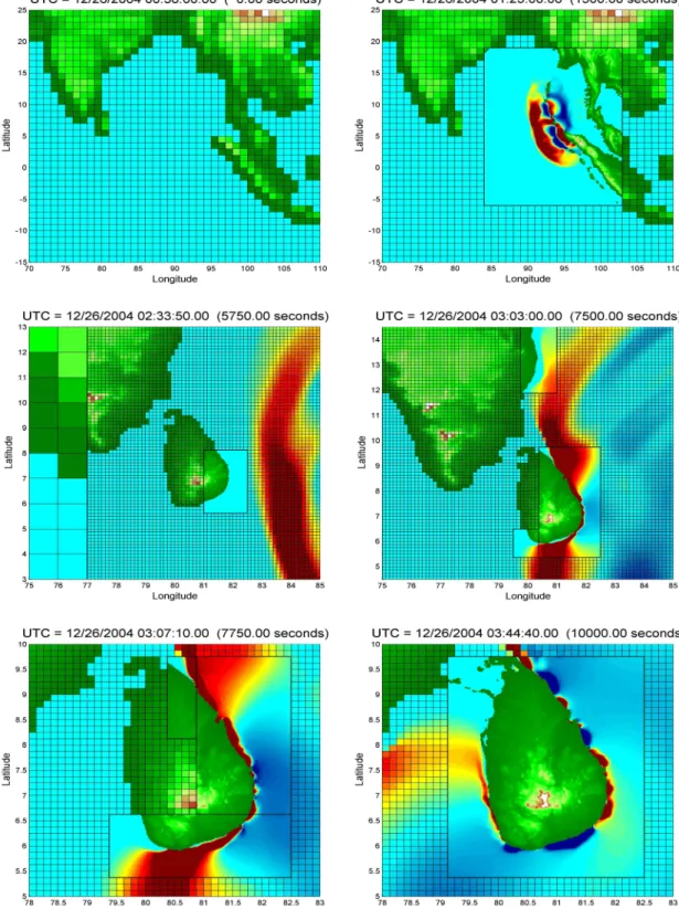
We are currently using our adaptive code to model the Indian Ocean tsunami of 2004. The tsunami is numerically generated by dynamically moving the seafloor according to a temporal-spatial model of the Sumatra-Andaman fault rupture, provided by the Seismolab at Caltech [1]. An example simulation is shown in Figure 1. This simulation used 40×40, 1◦×1◦grid cells on the coarsest grid (top left). A second level refined by a factor of 8, was used to track the deep ocean tsunami propagation (top right). Third level grids, allowed near Sri Lanka and the eastern coast of India, were again refined by a factor of 8, resulting in approximately 1 minute grid cells. Grid lines are omitted from these levels for clarity. This calculation ran in 28 minutes of computing time on a personal single processor Dell desktop.
We have used higher level grids in some regions allowing resolution onto 25 me-ter grid cells for inundation modeling. Because of the limited availability of digital bathymetry in the Indian Ocean region, we have had to manually digitize nautical charts in these regions—a process that is time consuming and labor intensive.
ACKNOWLEDGEMENTS
References
[1] C.J. Ammon et al. Rupture process of the 2004 Sumatra-Andaman earthquake. Science, 308:1133–1139, 2005.
[2] D. Bale, R. J. LeVeque, S. Mitran, and J. A. Rossmanith. A wave-propagation method for conservation laws and balance laws with spatially varying flux functions. SIAM J. Sci. Comput., 24:955–978, 2002.
[3] M. J. Berger and R. J. LeVeque. Adaptive mesh refinement using wave-propagation algorithms for hyperbolic systems. SIAM J. Numer. Anal., 35:2298–2316, 1998.
[4] G. Carrier, T. Wu, and H. Yeh. Tsunami run-up and draw-down on a plane beach. Journal of Fluid Mech., 475:79–99, 2003.
[5] D.L. George. Finite volume methods and adaptive refinement for tsunami propaga-tion and inundapropaga-tion. PhD thesis, University of Washington, 2006.
[6] T. Hou and P. LeFloch. Why non-conservative schemes converge to the wrong so-lutions: Error analysis. Math. of Comput., 62:497–530, 1994.
[7] R. J. LeVeque. The CLAWPACK software package.
http://www.amath.washington.edu/ claw.
[8] R. J. LeVeque. Balancing source terms and flux gradients in high-resolution Go-dunov methods: The quasi-steady wave propagation algorithm. Journal of Compu-tational Physics, 146:346–365, 1998.
[9] R. J. LeVeque. Finite Volume Methods For Hyperbolic Problems. Cambridge Uni-versity Press, 2002.
[10] R. J. LeVeque and D. L. George. High-resolution finite volume methods for the shal-low water equations with bathymetry and dry states. In P. Liu, editor, Proceedings of Long-Wave Workshop, Catalina, page to appear, 2004.
[11] Charles L. Mader. Numerical Modeling of Water Waves. CRC Press, 2004.