Abstract
This paper shows and discusses a generic implementation of the global-local analysis toward generalized finite element method (GFEMgl). This implementation, performed into an academic computational platform, follows the object-oriented approach presented by the authors in a previous work for the standard version of GFEM in which the shape functions of finite elements are hierarchically enriched by analytical functions, according to the problem behavior. In global-local GFEM, however, the en-richment functions are constructed numerically from the solution of a local problem. This strategy allows the use of a coarse mesh even when the problem produces complex stress distributions. On the other hand, a local problem is defined where the stress field presents high gradients and it is discretized using a large number of elements. The results of the local problem are used to enrich the global problem which improves the approximate solution. The great advantage is allowing a well-refined description of the local problem, when necessary, avoiding an overburden for the compu-tation of the global solution. Details of the implemencompu-tation are presented and important aspects of using this strategy are high-lighted in the numerical examples.
Keywords
Generalized finite element method, eXtended finite element meth-od, Object-oriented programming, Global-local, Enrichment func-tion
An Object-Oriented Class Organization for Global-Local
Generalized Finite Element Method
1 INTRODUCTION
Finite element method (FEM) is a powerful method to solve various physical problems. This meth-od is robust and has been thoroughly developed to solve engineering and applied science problems such as linear and non-linear stress analysis of solid and structures, electromagnetism, fluid flows
Mohammad Malekan a Felício B. Barros b Roque L. S. Pitangueira c Phillipe D. Alves d
a Graduate Program in Structural
Engineering (PROPEEs), School of Engineering, Federal University of Minas Gerais (UFMG), Belo Horizonte, MG, Brazil, [email protected]
d Department of Civil and Environmental
Engineering, University of Illinois at Urbana-Champaign, 205 North Mathews Avenue, Urbana, IL, USA,
http://dx.doi.org/10.1590/1679-78252832
and similar fields. In generalized finite element method (GFEM), Melenk and Babuška (1996), Strouboulis et al. (2000a), Duarte et al. (2000), Strouboulis et al. (2001), as in FEM, the approxi-mation is built over a mesh of elements using interpolation functions. However, the approxiapproxi-mation is associated with nodal points as in the Meshless methods, and it is enriched in the same fashion as in the hp-cloud method, Duarte et el. (1995), Duarte (1996), Liszka et al. (1996), Oden et al. (1998). Special functions multiply the original FEM functions and smooth and non-smooth solutions can be modeled independently of the mesh. The enrichment strategy of GFEM is similar to the one used in the extended finite element method (XFEM), introduced in Belytschko and Black (1999).
Global-local FEM was proposed by Noor (1986) in order to solve non-linear problems. This method was presented after proposing zooming method by Hirai et al. (1985). A local problem is defined where a local phenomenon happens. The global-local FEM approach has two steps. The first step is done with a coarse FEM mesh that ignores the effect of the local phenomena. This is fol-lowed by the second step which includes an analysis of the local region using refined finite element meshes. The key parameter for the local analyses is the application of field state variables as bound-ary conditions on the local boundaries. Once the solution of local problem is obtained, the global-local FEM analysis can be finished. In global-global-local GFEM (GFEMgl), Duarte et al. (2007), a varia-tion of the standard GFEM, enrichment funcvaria-tions are constructed numerically from the soluvaria-tion of a local problem. GFEMgl approach has three steps, its first and second steps are the same as the global-local FEM. In the third step, the results of the local problem are used to enrich the global problem which improves the approximate solution. In the case of fracture mechanic problems, the stress field around the crack tip presents high gradients and it is discretized using a large number of elements. The great advantage is providing a well-refined description of the local problem. More information on global-local GFEM, considering its various aspects can be found in Duarte and Kim (2008), Kim et al. (2008), Kim et al. (2009), Kim et al. (2010), Pereira et al. (2011), Gupta et al. (2012), Kim et al. (2012), Gupta et al. (2013), Evangelista et al. (2013), Plews and Duarte (2015).
formulations of global-local GFEM is presented. The INSANE class organization and its expansion to include GFEMgl method are discussed in section 4. In the section 5, numerical examples are pre-sented, and final section is devoted to concluding remarks and discussion.
2 THE GENERALIZED FINITE ELEMENT METHOD
A brief explanation of GFEM is described in this section. Further details can be found in Melenk and Babuška (1995), Babuška and Melenk (1997), Oden et al. (1998), Duarte et al. (2000), Strou-boulis et al. (2001), Pereira et al. (2011). The GFEM was developed for modeling structural prob-lems with discontinuities. The origins of this method can be summarized as:
• Research done by Babuška and co-workers – initially named as special finite element method by Babuška et al. (1994) and later as partition of unity method (PUM) by Melenk and Ba-buška (1996).
• Then, as a meshless formulation in the hp-cloud method, Duarte et al. (1995), and later as a hybrid approach with the FEM, Oden et al. (1998).
Furthermore, it can be considered an instance of the PUM, in the sense that it employs a set of PU functions to guarantee interelement continuity. Such strategy creates conforming approxima-tions which are improved by a nodal enrichment scheme. This basic idea shares the same character-istics from XFEM proposed by Belytschko and Black (1999), as it is observed in Fries and Be-lytschko (2010).
Here this procedure is summarized following Barros et al. (2004, 2013) and considering two-dimensional space. A conventional finite elements mesh can be considered for which is a set of NE elements, defined by N nodes, .
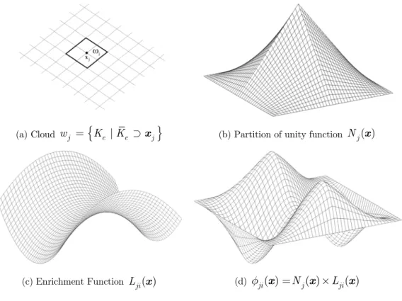
A generic patch of elements or cloud wj Î W is obtained by the union of finite elements sharing
the vertex node xj, Fig. 1(a). The assemblage of the interpolation functions, built at each element
e j
K Îw and associated with node xj, composes the function Nj( )x defined over the support
cloud wj. As
1 ( ) 1
N j
j= N =
å
x at every point x in the domainW, the set of functionsconstitutes a partition of unity (PU). A set of q linearly independent functions is defined at each cloud wj as:
1 2 1 1
{ ( ), ( ),..., ( )} { ( )}q ( ) 1
j j j jq ji i j
I = L x L x L x = L x = L x = (1)
The generalized finite element shape functions are determined by the enrichment of the PU functions, which is obtained by the product of such functions by each one of the components of the set Ij at the generic cloud wj:
1 1
{ }q ( ) { ( )}q ji i Nj Lji i
f = = x ´ x = (2)
approximation (also called enrichment function). The resulting shape function, fji( )x , Fig. 1(d), inherits characteristics of both functions, i.e., the compact support and continuity of the PU and the approximate character of the local function.
(a) Cloud wj =
{
Ke |Ke Éxj}
(b) Partition of unity function ( )j
N x
(c) Enrichment Function Lji( )x (d) fji( )x =Nj( )x ´Lji( )x
Figure 1: Enrichment scheme for a cloud wj, from Barros et al. (2007).
As a consequence, the generalized global approximation, denoted by u( )x , can be described as a linear combination of the shape functions associated with each node:
= =
é ù
= ê + ú
ë û
å
å
( ) Nj 1Nj( ) j qi 2Lij( ) ji
u x x u x b (3)
where uj and
ji
b are nodal parameters associated with standard – ( )
j
N x – and GFEM –
( ) ( )
j ji
N x ´L x – shape functions, respectively. Aiming to minimize round-off errors, Duarte et al. (2000) suggest that a transformation should be performed over the Lji( )x functions, if they are of polynomial type. In such case, the coordinate x is replaced as follows:
j
j
h -x x
x (4)
3 GLOBAL-LOCAL GENERALIZED FINITE ELEMENT METHOD
This method, originally proposed by Duarte and Babuška (2005), combines the standard GFEM with the global-local strategy proposed by Noor (1986). GFEMgl is suitable for problems with local phenomena, such as stress field next to the crack tip. The analysis is divided in three steps: initial global problem (step 1), local problem (step 2) and final global problem (step 3). These steps are described in the following sub-sections.
3.1 Initial Global Problem (Step 1)
Following Kim et al. (2010), consider a domain W = W È ¶WG G G of an elastic problem inRn. The
boundary is decomposed in u
G G G
s
¶W = ¶W È ¶W with ¶W Ç ¶W = Æu
G G
s , where indices u and s
refer to the Dirichlet and Neumann boundary conditions. 0 0( )
G Î G WG
u X represents the solution of
the approximate space 0( )
G WG
X (built by FEM or GFEM functions) for the initial global problem in its weak form, shown in:
0 0 0
( ) : ( ) .
G G
G G d s Gd
W ¶W
ò
su ev x =ò
t v s (5)where , , 0 0( )
G Î G WG
v X
s e , and t are stress tensor, strain tensor, test functions, and prescribed traction vector, respectively.
3.2 Local Problem (Step 2)
L
W is a sub-domain from WG. This sub-domain may contain cracks, holes or other special features, as suggested by Duarte and Kim (2008). The corresponding local solution E( )
L Î L WL
u X is
ob-tained from: s s s \( ) 0 0 \( ) ( ) : ( ) . . . . ( ( ) ). u u
L L G L L G L G
u
L G L L G
L L L L L L L
L G G L
d d d d
d d
s
h k
h k
W ¶W ǶW ¶W ¶W ǶW ¶W ǶW
¶W ǶW ¶W ¶W ǶW
+
+ +
ò
ò
ò
ò
ò
ò
su ev x + u v s + u v s = t v
u v t u u v
(6)
where E( )
L Î L WL
v X represents the test functions, E( )
L WL
X is the space generated by FEM or
GFEM functions, h is the penalty parameter and k is the stiffness parameter both used to impose Dirichlet and Cauchy boundary conditions, respectively. Additionally, t is the prescribed traction, u is the prescribed displacement, t u( G0) is the traction vector obtained from the first step. ¶WL \ (¶W Ç ¶WL G) is the part of the local problem boundary that doesn't coincide with the global problem boundary and on which the numerical solution that comes from the step 1 is im-posed as boundary condition. The last integrals on the left and right side of Eq. (6) correspond to the Cauchy or spring boundary condition, imposing the displacements as well as the stress calculat-ed in the global problem. The E( )
L WL
1
ˆ
( ) ( ) ( ) ( ) ( ) ( )
L
N
E E E E
L L j j j j
j N H = ì ü ï ï ï ï
ï é ùï
W =íï = êë + + úûýï
ï ï
ï ï
î
å
þ
X u x x u x u x u x (7)
functions uˆ ( ),Ej x HuEj ( )x and E( ) j
u x are continuous, discontinuous and singular components of the
approximate solution and Nj is the partition of unity function used in global problem. The number
of nodes of the local domain is given by NL.
3.3 Final Global Problem (Step 3)
The global problem is enriched by solution uL (from step 2). The new solution E E( )
G Î G WG
u X is
obtained from:
( ) : ( ) .
G G
E E E
G G d s Gd
W ¶W
ò
su ev x =ò
t v s (8)where E G
v represents the test functions and E( )
G WG
X is the initial space increased by gl( )
k
u x from
local problem uL:
1 ˆ
( ) ( ) ( ) ( ) ( ) ( )
gl
N gl
E E
G G j j j k k
k I N N = Î ì ü ï ï ï ï ï ï
W =íï = + ýï
ï ï
ï ï
î
å
å
þ
X u x x u x x u x (9)
and k ÎIgl represent the set of nodes enriched by the local solution uL.
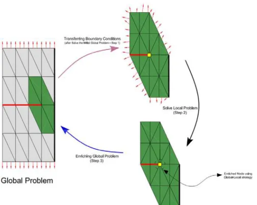
Figure 2 illustrates a simplified global-local strategy. First the initial global problem is solved using a coarse mesh. After defining the local domain, the results of the initial global problem is transferred as a boundary condition to the local problem. Finally, the solutions of the local problem are transferred to the final global problem as a numeric enrichment function in order to enrich the predefined nodes of the global problem.
4 INTERACTIVE STRUCTURAL ANALYSIS ENVIRONMENT
Figure 2: Three steps of the Global-Local strategy.
The INSANE numerical core is composed by the interfaces Assembler, Model and Persistence and the abstract class Solution. Figure 3 shows the unified modeling language (UML) diagram from numerical core of INSANE.
The observation strategy is determined by the observer-observable design pattern, which is a change propagation mechanism. When an object of type observer (which implements the interface
java.util.observer) is instantiated, it is added to a list of observers of other objects of type
observa-bles (which extends the class java.util.observable). Any modification in the state of an observed object notifies the corresponding observer object that updated itself.
Detailed of GFEM implementation can be found in Alves et al. (2013), section 4. Here, the fo-cus is on the main modifications in order to expand the computational system to comprise GFEMgl. Following sub-sections explain various INSANE classes and approaches in order to perform GFEM analysis as well as GFEMgl analysis.
4.1 Persistence Interface
Persistence treats the input data and persists the output data. For GFEMgl, this class was extended
to deal with more than one model. In that case, the data is separated in a global model and several local models, corresponding to the global and the several local problems respectively.
4.2 Assembler Interface
Assembler interface is responsible for assembling the linear equation system provided by the
dis-cretization of the initial value problem. This class is implemented following the generic representa-tion:
+ + =
AX BX CX D (10)
where X is the solution vector; the single dot represent its first time derivative and the double dots its second time derivative; A, B and C are matrices with the properties of the problem and D is a vector that represents the system excitation.
The Assembler interface has the necessary methods for assembling the matrix system. It is
im-plemented by an object of the class GFemAssembler that was modified in order to transfer bounda-ry condition from the global model to the several local models. A Cauchy boundabounda-ry condition was implemented following Kim et al. (2010) (here represented by Eq. (6)).
In static analysis, Eq. (10) is simplified by eliminating the two first terms. The resulting matrix system is:
uu up u p
pu pp p u
é ù ìïï üïï ìïï üïï ê úí ý=í ý
ê ú ï ï ï ï
ê ú ï ï ï ï
ë û î þ î þ
C C X D
C C X D (11)
4.3 Solution
Solution abstract class starts the solution process and has the necessary resources for solving the
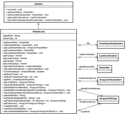
matrix system. GFEMgl process is implemented by GlobalLocal class, as shown in Fig. 4. Since GFEMgl is composed by more than one model (one global model and several local models), the problem has more than one assembler, each one responsible to build the corresponding equation in the form of (11). This is the main difference from standard GFEM solution class. Figure 4 shows in details the UML diagram for this class.
Figure 4: UML diagram for Solution class.
The main attributes of this class are:
− globalPath: contains the path of the file responsible for storing the global model description.
− solverType: contains information about the type of solver of the linear equation system.
− leq: LinearEquationSystem object which is responsible to solve the linear equation system.
− loadCombination: load combination of the problem.
− globalAssembler: handles information about the global model.
− localAssemblerList: list of Assembler objects that handles information about the several local
models.
− globalEnrichedNodes: handles the pointer to the global nodes that will be enriched by
− localEnrichedList: list that relates each global node, that will be enriched by the global-local enrichment strategy, with the corresponding local model. This is a very important infor-mation because it is in the local model that the function ukgl( )x will be built and used to en-rich the PU of the global node.
− localPath: contains the list of paths of each file responsible for storing each local model
de-scription.
4.4 Model Interface
The Model interface contains the data of the discrete model and provides to Assembler information
to assemble the final matrix system. Both Model and Solution communicate with the Persistence interface, which treats the input data and persists the output data to the other applications, when-ever it observes a modification of the discrete model state. This interface consisted of the following classes:
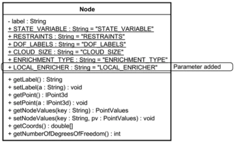
4.4.1 Node
This class is designed to manage the geometric representation of a node entity as well as the infor-mation from the discrete model. In addition to inforinfor-mation about the node coordinates, this class holds lists of identifiers such as type of degrees of freedom, state variables and type of nodal con-straint. This list of identifiers are based on HashMap strategy provided by JAVA API Collection Horstmann and Cornell (2008). This type of Java storing strategy allows an indirect communication between variables associated to the Node, named keys, and the variables stored in the Model. In spite of degrading performance of the framework, such strategy creates a generic and friendly im-plementation because it simplifies how new information is added to the class. Furthermore, methods from JAVA API Collection allows using the keys like conventional attributes which preserves the readability of the code. “LOCAL_ENRICHER” is added in order to indicate which local domain will provide the global-local enrichment function, as shown in Fig. 5. This new attribute is defined in the Node class as an instance of GFEM using the enrichment strategy.
4.4.2 Element
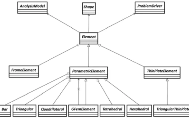
In Alves et al. (2013), this class was not modified for standard GFEM. On the other hand, the spe-cial characteristics of GFEMgl, such as the relationship between the global and the local elements, requires a new extension of the Element class. Note that this new GFemElement class is not only derived from the superclass Element but also contains on object of Element type, Fig. 6.
Figure 6: UML diagram for Element class.
Indeed this strategy takes advantage of parametric element library, with bar, triangular, quadri-lateral, tetrahedral and hexahedral elements, without having to use simple inheritance from each one of those types of elements. Figure 7 shows the new parameters added in GFemElement class in order to add the ability to solve problems using the global-local scheme. Similar to the Node class,
the HashMap strategy is used to include new parameters. The parameters of this class are:
− LOCAL_NAME: if the element belongs to a local problem, this parameter indicates in which
local model it is inserted.
− GLOBAL_ELEMENT: if the element belongs to a local problem, this parameter indicates
which element from the global model contains the current element. This relationship allows to obtain from the global element the necessary data to apply the boundary conditions on the edge, if it is the case, of the current element.
− LOCAL_ELEMENTS: if the element belongs to a global problem, this parameter indicates
the elements of the local problem that discretize the domain of this global element. In this implementation the local mesh is nested in the global mesh. As a consequence each global el-ement exactly contains a set of local elel-ements.
− BOUNDARY_INFORMATION: informs which kind of boundary conditions is transferred
from step 1 to step 2.
− STEP_GL: informs in which step of the problem the solution is being processed.
− LOCAL_TWINS: if the element belongs to a local problem, this parameter indicates which
Figure 7: UML diagram for GFemElement class.
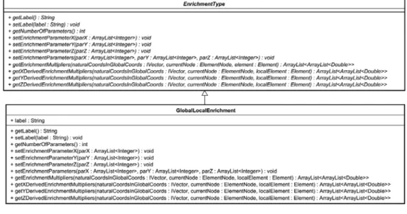
4.4.3 EnrichmentType
GlobalLocalEnrichment extends EnrichmentType and provides specific methods to build the
en-riched functions from the solution of the local problem and applied in the third step of the global-local problem. Figure 8 shows the class diagram of this class. EnrichmentType is an abstract class and its methods are abstract. Thus, GlobalLocalEnrichment class contains the same method as the
EnrichmentType class.
Figure 8: UML diagram for GlobalLocalEnrichment.
4.4.4 Problem Driver
Figure 9: Sequence diagram for stiffness calculation.
4.5 Generic Boundary Condition
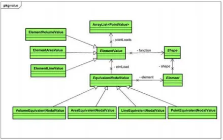
Figure 10 shows the relationship between the types of objects found in the package Value, which is used to define a generic boundary condition of the problem (e.g., conditions of Dirichlet, Neumann or Cauchy required by Eq. (6)). The definition of these boundary conditions in different geometric entities is performed through an ElementValue object, which is derived for the specific types
Ele-mentVolumeValue (boundary conditions applied in a volume), ElementAreaValue (boundary
condi-tions applied to a area) and ElementLineValue (boundary conditions imposed on a line).
Ele-mentValue consists of the following attributes:
− An array of objects of type PointValue, responsible for storing the coordinates of a point and information that defines the boundary condition at this point.
− An object of type Shape, responsible for the interpolation of PointValue.
The class Shape is responsible for providing the approximation function that interpolates the different PointValue applied in a region of the element that can be a line, area or a volume, depend-ing on the element type. The responsible for combindepend-ing this information and providdepend-ing the equiva-lent nodal value is EquivalentNodalValue class, whose attributes are objects of Element and
Ele-mentValue classes.
4.6 Information Transferring from the Global to the Local Problem
One of the actions performed during the process of generalization of the imposition of boundary conditions on INSANE environment is to add the ability to obtain boundary conditions of an ele-ment of the local problem from an eleele-ment of the global problem. This is required in the global-local analysis process in which, it is necessary to impose boundary conditions for the global-local problem provided by the global mesh solution. There are basically three types of boundary conditions that can be used:
– Dirichlet boundary conditions – Neumann boundary conditions – Cauchy boundary conditions
The class responsible for the transfer of boundary conditions between domains is the
Equiva-lentNodalValue class that is part of the Value package. The EquivalentNodalValue class has
meth-ods that fall into those capable of modifying the matrix C (stiffness) and those able to modify the vector D (force) of the system in Eq. (10), as can be seen in Fig. 11.
Figure 11: EquivalentNodalValue class.
5 NUMERICAL EXAMPLES
are very simple, since the goal is not demonstrate the capabilities of the methods, but the general approach proposed to enclose the GFEMgl formulation in INSANE environment.
Among the three aforementioned boundary conditions in section 4.6, according to Kim et al. (2010), the Dirichlet boundary conditions (a limiting case of Cauchy boundary condition) lead to worse results than Cauchy boundary conditions. Thus, for all two examples, the Dirichlet boundary conditions are applied on the local problem boundaries in order to demonstrate the robustness of the methodology in the worst case scenario.
Numerical integration for the first and second steps of the global-local analysis is done based on standard Gaussian quadrature procedure. In the third step, the numerical integration for those global elements that contain local elements is done over the Gauss points of local elements, as pro-posed by Kim et al. (2010). Consider that a global element contains nLe local elements and number of Gauss points for each local elements be equal to GP. Thus, the number of integration points for this global element is obtained by:
1 Le
n i i= GP
å
. In other words, the global numerical integration is done over Gauss points of each local element that represent a part of the global element.5.1 Linear Bending-Moment Problem
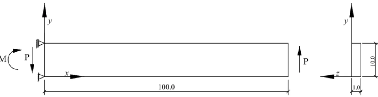
Figure 12 illustrates a beam subjected to a set of loads that produce a linear-bending moment. In Lee and Bathe (1993), this problem is used to evaluate numerically the effects of element distortions in FEM. Here, this problem exemplifies and validates the GFEMgl implementation within INSANE environment.
Figure 12: Linear bending-moment problem - geometry and loading.
The data for solving this two-dimensional plane stress problem are (using consistent units):
− Modulus of elasticity E = 1.0 × 10⁷;
− Poisson ratio ν = 0.3;
− Load P = 20 distributed as the load function fy = 0.12y2+ 1.2y. − Moment M = 2000 distributed as the load function fx = 24y–120.
2 3 2 2
1
(0.12 0.092 y 0.6 24 1.38 120 4.6 )
u x x xy y x y
E
= - - - + + - (12)
3 2 2 2
1
( 0.04 0.036 y 12 0.36 3.6 4.6 36 )
v x x x xy y x y
E
= - - + + + + - (13)
Using the GFEMgl, the solution of this problem can be divided in three steps:
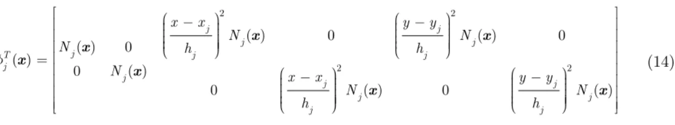
• Step 1: All the nodes of the problem are enriched by P2 functions (quadratic enrichment).
This strategy guarantees a cubic order of approximation through the beam, reproducing the analytical solution of the problem (see Eqs. (12) and (13)). The P2 enrichment function for x direction is as follows:
2 2
2 2
( ) 0 ( ) 0
( ) 0 ( )
0 ( )
0 ( ) 0 ( )
j j
j j
j
T j j
j
j
j j
j j
j j
x x y y
N N
N h h
N x x y y
N N h h f - -= -
-é æ ö æ ö ù
ê çç ÷÷ çç ÷÷ ú
ê çç ÷÷÷ çç ÷÷÷ ú
ê è ø è ø ú
ê ú
ê æ ö æ ö ú
ê çç ÷÷ çç ÷÷ ú
ê çç ÷÷÷ çç ÷÷÷ ú
ê è ø è ø ú
ë û x x x x x x x (14)
• Step 2: Global problem is split in 9 local problems, as presented in Fig. 13. Each local
prob-lem is enriched using P2 functions in order to exactly represent the analytical solution of the problem (this is only possible if exact boundary conditions are provided from step 1). At the end of step 2, there is a numerical solution that can exactly reproduce this problem.
• Step 3: Returning to the global problem, the enrichment P2 is replaced by global-local
en-richment obtained from step 2. For this example, the numerical solution from local problems can exactly reproduce the analytical solution for this problem.
For this analysis, a Gauss-Legendre quadrature rule with 4 × 4 points is employed for both global and local problems.
Figure 14 shows stress distribution of stress component σxx for each local domain of the beam.
(a) Local domain 1 (cloud of node 1)
(b) Local domain 2 (cloud of node 3)
(c) Local domain 3 (cloud of node 7)
(d) Local domain 4 (cloud of node 9)
(e) Local domain 5 (cloud of node 2)
(f) Local domain 6 (cloud of node 8)
(g) Local domain 7 (cloud of node 4)
(h) Local domain 8 (cloud of node 6)
(i) Local domain 9 (cloud of node 5)
(a) σxx for local 1 (b) σxx for local 2
(c) σxx for local 3 (d) σxx for local 4
(e) σxx for local 5 (f) σxx for local 6
(g) σxx for local 7
(h) σxx for local 8
(i) σxx for local 9
Figure 14: Results of stress component σxx for each local domain.
5.2 Fracture Mechanic Problem
− Modulus of elasticity E = 1.0;
− Poisson ratio ν = 0.3;
− Traction σ = 1.0.
Figure 15: Geometry and loading of a cracked plate submitted to an axial stress.
The reference solution of this problem is obtained using a mesh of 12087 p–quadrilateral ele-ments in ANSYS®. For GFEMgl analysis, however, a smaller number of finite elements as well as of degrees of freedom (DOFs) is used. The reason for using a smaller number of DOFs is explained by the use of global-local enrichment function, which is suitable for high stress concentration. This strategy is used to describe the singular stress near the crack tip.
A geometric mesh is used to describe the local domain, Fig. 16 and it is shown in Fig. 17. This mesh is graded so that the elements are decreased in geometric progression toward the crack tip, in four levels (L1, L2, L3 and L4) with a common reduction factor of 10%. Results are shown in Fig. 18. Also, Table 1 presents a comparison between the strain energy values for the reference and ap-proximate solutions.
Analysis DOFs Strain energy
Reference result 24648 10.98326
Global-local result 134 10.80963
Table 1: DOFs and strain energy for geometric enrichment.
It can be observed from the results shown in Fig. 18 and Table 1 the capability of the global-local enrichment strategy to represent the singular stress field close to the crack tip.
Figure 17: Geometric mesh with reduction rate f = 10%.
Figure 18: Results for stress component σxx (step 3) in different positions given by the coordinate x
6 CONCLUSION
An overview of the GFEMgl is given with emphasis on implementation aspects under OOP ap-proach. The focus of this work is to present a GFEMgl extension of a FEM programming environ-ment called INSANE. The proposed approach allows to combine any types of partition of unity methods, analysis model and enrichment strategy. Also, an expansion of the numerical core IN-SANE, in order to adapt it to impose boundary conditions using the penalty method is included. The OOP approach is fully exploited, reinforcing the premise segmentation and encapsulation of the INSANE environment. The validation of this extension and some additional conclusions about the GFEM global-local strategy are presented by numerical examples for Solid Mechanics.
Acknowledgments
The authors would like to gratefully acknowledge the important support of the Brazilian research agencies CNPq (National Council for Scientific and Technological Developments - Grants 309005/2013-2, 486959/2013-9 and 308785/2014-2), FAPEMIG (Foundation for Research Support of the State of Minas Gerais - Grant PPM-00669-15) and CAPES (Coordination for the Improvement of Higher Education Personnel).
References
Alves, P.D., Barros, F.B., Pitangueira, R.L.S. (2013). An object oriented approach to the generalized finite element method, Advances in Engineering Software 59: 1–18.
Babuška, I., Caloz, G., Osborn, J. E. (1994). Special finite element method for a class of second order elliptic prob-lems with rough coefficients, SIAM J. Numerical Analysis 31(4): 745–981.
Babuška, I., Melenk, J.M. (1997). The partition of unity method, International Journal of Numerical Methods in Engineering 40: 727–58.
Barros, F.B., de Barcellos, C.S., Duarte, C.A. (2007). p-Adaptive Ck generalized finite element method for arbitrary polygonal clouds, Computational Mechanics 41: 175–87.
Barros, F.B., de Barcellos, C.S., Duarte, C.A., Torres D.F. (2013). Sub-domain based error techniques for generalized finite element approximations of problems with singular stress fields, Computational Mechanics 52: 1395–415. Barros, F.B., Proença, S.P.B., de Barcellos, C.S. (2004). On error estimator and p-adaptivity in the generalized finite element method, International Journal of Numerical Methods in Engineering 60(14): 2373–98.
Belytschko, T., Black, T. (1999). Elastic crack growth in finite elements with minimal remeshing, International Journal of Numerical Methods in Engineering 45: 601–20.
Bordas, S., Nguyen, P.V., Dunant, C., Guidoum, A., Nguyen-Dang, H. (2007). An extended finite element library, International Journal of Numerical Methods in Engineering 71: 703–32.
Chamrová, R., Patzák, B. (2010). Object-oriented programming and the extended finite-element method, Proc. Inst. Civ. Eng. - Eng. Computational Mechanics 163: 271–78.
Duarte, C. A. (1996). The hp-cloud method, PhD dissertation, University of Texas at Austin, USA.
Duarte, C.A., Babuška, I. (2005). A global-local approach for the construction of enrichment functions for the gfem and its application to propagating three-dimensional cracks, ECCOMAS Thematic Conference on Meshless Methods. Duarte, C.A., Babuška, I., Oden, J.T. (1995). Hp clouds - A meshless method to solve boundary-value problem, Tech. rep., TICAM, The University of Texas at Austin, technical Report.
Duarte, C.A., Kim, D.J. (2008). Analysis and applications of a generalized finite element method with global-local enrichment functions, Computer Methods in Applied Mechanics and Engineering 197: 487–504.
Duarte, C.A., Kim, D.J., Babuška, I. (2007). A global-local approach for the construction of enrichment functions for the generalized fem and its application to three-dimensional cracks, in: V. L. Ao, C. Alves, C. A. Duarte (eds.), Adv. Mesh. Tech., 1–26.
Dunant, C., Vinh, P.N., Belgasmia, M., Bordas, S., Guidoum, A. (2007). Architecture tradeoffs of integrating a mesh generator to partition of unity enriched object-oriented finite element software, Revue Europ. de Mécanica Numérico 16(2): 237–58.
Evangelista, F., Roesler, J.R., Duarte, C.A. (2013). Two-scale approach to predict multi-site cracking potential in 3-d structures using the generalized finite element method, International Journal of Solids and Structures 50: 1991–2002. Fonseca, F.T., Pitangueira, R.L.S. (2007). An object oriented class organization for dynamic geometrically non-linear, Tech. rep., CMNE (Congress on Numerical Methods in Engineering)/CILAMCE 2007, Porto, 13-15 June, Portugal.
Fries, T.P., Belytschko, T. (2010). The extended/generalized finite element method: An overview of the method and its applications, International Journal of Numerical Methods in Engineering 84(3): 253–304.
Gupta, V., Kim, D.J., Duarte, C.A. (2012). Analysis and improvements of global-local enrichments for the general-ized finite element method, Computer Methods in Applied Mechanics and Engineering 245-246: 47–62.
Gupta, V., Kim, D.J., Duarte, C.A. (2013). Extensions of the two-scale generalized finite element method to nonline-ar fracture problems, International Journal for Multiscale Computational Engineering 11(6): 581–96.
Hirai, I., Uchiyama, Y., Mizuta, Y., Pilkey, W.D. (1985). An exact zooming method, Finite Elements in Analysis and Design 1: 61–9.
Horstmann, C.S., Cornell, G. (2008). Core Java - Volume I - Fundamentals, vol. 1, 8th ed., Sun Microsystems Press. Kim, D.J., Duarte, C.A., Pereira, J.P. (2008). Analysis of interacting cracks using the generalized finite element method with global-local enrichment functions, ASME Journal of Applied Mechanics 75: 763–813.
Kim, D.J., Duarte, C.A., Proença, S.P.B. (2009). Generalized finite element method with global-local enrichments for nonlinear fracture analysis, International Symposium on Mechanics of Solids in Brazil, H.S.C. Mattos and M. Alves (Editors), 317–30.
Kim, D.J., Duarte, C.A., Proença, S.P.B. (2012). A generalized finite element method with global-local enrichment functions for confined plasticity problems, Computational Mechanics 50: 1–16.
Kim, D.J., Pereira, J.P., Duarte, C.A. (2010). Analysis of three-dimensional fracture mechanics problems: A two-scale approach using coarse generalized fem meshes, International Journal of Numerical Methods in Engineering 81: 335–65.
Lee, N.S., Bathe, K.J. (1993). Effects of element distortions on the performance of isoparametric elements, Interna-tional Journal of Numerical Methods in Engineering 36: 3553–76.
Liszka, T.J., Duarte, C.A., Tworzydlo, W.W. (1996). hp-meshless cloud method, Computer Methods in Applied Mechanics and Engineering 139: 263–88.
Melenk, J.M., Babuška, I. (1995). The partition of unity finite element method, Technical Report BN-1185, Inst. for Phys. Sci. Tech., University of Maryland, USA.
Melenk, J.M., Babuška, I. (1996). The partition of unity finite element method: Basic theory and applications, Com-puter Methods in Applied Mechanics and Engineering 39: 289–314.
Melenk, J.M., On generalized finite element methods, PhD dissertation, University of Maryland, College Park (1995). Neto, D.P., Ferreira, M.D.C., Proença, S.P.B. (2013). An object-oriented class design for the generalized finite ele-ment method programming, Latin American Journal of Solids and Structures 10(6): 1267–91.
Noor, A.K. (1986). Global-local methodologies and their application to nonlinear analysis, Elements in Analysis and Design 2: 333–46.
Oden, J.T., Duarte, C.A., Zienkiewicz, O.C. (1998). A new cloud-based hp finite element method, Computer Meth-ods in Applied Mechanics and Engineering 153:117–26.
Pereira, J.P., Kim, D.J., Duarte, C.A. (2011). A two-scale approach for the analysis of propagating three-dimensional fractures, Computational Mechanics 49(1): 99–121.
Plews, J.A., Duarte, C.A. (2015). Bridging multiple structural scales with a generalized finite element method, Inter-national Journal of Numerical Methods in Engineering 102(3-4): 180–201.
Strouboulis, T., Babuška, I., Copps, K. (2000a). The design and analysis of the generalized finite element method, Computer Methods in Applied Mechanics and Engineering 181(1-3): 43–69.