The Hamiltonian Alternating Path Problem
Anna Gorbenko, Vladimir Popov
Abstract—In this paper, we consider the Hamiltonian alter-nating path problem for graphs, multigraphs, and digraphs. We describe an approach to solve the problem. This approach is based on constructing logical models for the problem. We use logical models for the Hamiltonian alternating path problem to solve the Hamiltonian path problem and the planning a typical working day for indoor service robots problem. Also, we use these models for Bennett’s model of cytogenetics, automatic generation of recognition modules, and algebraic data.
Index Terms—Hamiltonian alternating path, Hamiltonian path, the planning a typical working day for indoor service robots problem, NP-complete, logical models.
I. INTRODUCTION
R
ECENTLY, a number of Hamiltonian problems for edge-colored graphs were considered (see e.g. [1], [2]). It should be noted that in the last years the concept of alternating trails and the special cases, alternating paths and cycles, appears in various applications (see e.g. [3], [4]). In particular, we can mention that some problems in molecular biology correspond to extracting Hamiltonian or Eulerian paths or cycles colored in specified pattern [5]–[7], transportation and connectivity problems where reload costs are associated to pair of colors at adjacent edges [8], social sciences [9], VLSI optimization [10], etc. Also, there are a number of applications in graph theory and algorithms.In this paper, we describe an approach to solve the Hamil-tonian alternating path problem for graphs, multigraphs, and digraphs. This approach is based on constructing logical models for the problem. Also, we consider an application of this approach to solve the Hamiltonian path problem and the planning a typical working day for indoor service robots problem [11].
II. PRELIMINARIES AND PROBLEM DEFINITIONS Multiple edges are edges that have the same end nodes. A multigraph is a set of nodes connected by edges which is permitted to have multiple edges. Thus, in multigraph, two vertices may be connected by more than one edge. In this paper, we consider only edge-colored multigraphs. We assume that each edge of a multigraph has a color and no two multiple edges have the same color. All multigraphs considered are finite and have no loops. When multigraphs have no multiple edges, we call them graphs, as usual. A digraph is a graph where the edges have a direction associated with them.
An edge of graph with vertices x and y we denote by
(x, y). In this case, we assume that (x, y) = (y, x). For multigraphs, an edge with vertices x and y we denote by
Ural Federal University, Department of Intelligent Systems and Robotics of Mathematics and Computer Science Institute, 620083 Ekaterinburg, Rus-sian Federation. Email: [email protected], [email protected]
The work was partially supported by Analytical Departmental Program ”Developing the scientific potential of high school” and Ural Federal Uni-versity development program with the financial support of young scientists.
z[x, y]. In this case, we assume that z1[x, y] = z2[x, y] if and only ifz1=z2. For digraphs, we assume that an edge (x, y)is considered to be directed fromxtoy. In this case, we assume that(x, y)6= (y, x).
If the number of colors is restricted by an integer c, we speak about c-edge-colored multigraphs. In this paper, we consider only simple paths and cycles. LetG be a c -edge-colored multigraph. A cycle or path inGis called alternating if its successive edges differ in color. An alternating path or cycle is called Hamiltonian if it contains all the vertices of
G. If G has a Hamiltonian alternating cycle, G is called Hamiltonian. An alternating pathP is called an(x;y)-path ifxandyare the end vertices of P. The alternating Hamil-tonian path problem and the alternating HamilHamil-tonian cycle problem are problems of determining whether an alternating Hamiltonian path or an alternating Hamiltonian cycle exists in a given multigraph.
III. THE ALTERNATINGHAMILTONIAN PATH PROBLEM FOR2-EDGE-COLORED MULTIGRAPHS
The alternating Hamiltonian path problem and the alternat-ing Hamiltonian cycle problem are extensively studied (see e.g. [3], [14]). However, the computational complexity of these problems are not quite clear. In [12], the authors noted that the alternating Hamiltonian cycle problem, even for 2-edge-colored graphs, is triviallyNP-complete. However, the authors of [12] have not given proof or any other evidence of this fact. In [3], the authors noted that problems on alternating cycles and paths in general 2-edge-colored graphs are at least as difficult as the corresponding ones for directed cycles and paths in digraphs. The authors of [3] gave the following motivation for this fact. “To see that, we consider the following simple transformation attributed to H¨aggkvist in [13]. LetDbe a digraph. Replace each arcxyofDby two (unoriented) edgesxzxyandzxyyby adding a new vertexzxy
and then colour the edgexzxy red and the edge zxyy blue.
LetGbe the 2-edge-coloured graph obtained in this way. It is easy to see that each alternating cycle inGcorresponds to a directed cycle inDand vice versa. Hence, in particular, the following problems on paths and cycles in 2-edge-coloured graphs are NP-complete: the Hamiltonian alternating cycle problem and the problem to find an alternating cycle through a pair of vertices.” It should be noted that the motivation is incorrect. For instance, we can consider the digraph
D1= ({1,2,3},{(1,2),(2,3),(1,3)}).
Using the transformation, we obtain the 2-edge-colored graph
G1= ({1,2,3, z12, z23, z13},
(z23,3),(1, z13),(z13,3)})
where
{(1, z12),(2, z23),(1, z13)}
is the set of red edges and
{(z12,2),(z23,3),(z13,3)}
is the set of blue edges. It is clear thatD1has a Hamiltonian
path. On the other hand, it is easy to check that G1 has no
alternating Hamiltonian path. Similarly, we can consider the digraph
D2= ({1,2,3,4},{(1,2),(2,3),(3,4),(4,1),(1,3)}).
Using the transformation, we obtain the 2-edge-colored graph
G2= ({1,2,3,4, z12, z23, z34, z41, z13},
{(1, z12),(z12,2),(2, z23),(z23,3),
(3, z34),(z34,4),(4, z41),(z41,1),
(1, z13),(z13,3)})
where
{(1, z12),(2, z23),(3, z34),(4, z41),(1, z13)}
is the set of red edges and
{(z12,2),(z23,3),(z34,4),(z41,1),(z13,3)}
is the set of blue edges. It is easy to see that that D2 has a
Hamiltonian cycle, butG2 is not Hamiltonian.
In our investigations, we need an explicit proof of hardness of the alternating Hamiltonian path problem. The proof of the following Proposition 1 gives us an explicit reduction from the Hamiltonian path problem to the alternating Hamiltonian path problem.
Note that the decision version of the alternating Hamil-tonian path problem for c-edge-colored multigraphs can be formulated as following.
THE ALTERNATING HAMILTONIAN PATH PROBLEM FOR
c-EDGE-COLORED MULTIGRAPHS(c-AHP-M):
INSTANCE: A c-edge-colored multigraph G = (V, E)
whereV is the set of vertices andE is the set of edges.
QUESTION: Does G have an alternating Hamiltonian path?
Proposition 1. 2-AHP-MisNP-complete.
Proof. It is clear that c-AHP-M is in NP. Therefore, we need to prove only NP-hardness of 2-AHP-M. Let us consider the following problem:
HAMILTONIAN PATH PROBLEM FOR GRAPHS(HP-G): INSTANCE: A graphD= (A, B).
QUESTION: DoesD have a Hamiltonian path?
HP-G is NP-complete (cf. [15]). Now, we transform an instance of HP-G into an instance of2-AHP-M as follows:
V =A,
E={r[x, y], b[x, y]|(x, y)∈B},
G= (V, E),
where
Er={r[x, y]|(x, y)∈B}
is the set of red edges and
Eb={b[x, y]|(x, y)∈B}
is the set of blue edges. It is clear that if
(x1, x2),(x2, x3), . . . ,(x|A|−1, x|A|)
is a Hamiltonian path inD, then
r[x1, x2], b[x2, x3], . . . , u[x|A|−1, x|A|],
where u = r for even |A| and u = b for odd |A|, is an alternating Hamiltonian path inG. By definition of G, it is easy to see that
u1[x1, x2], u2[x2, x3], . . . , u|A|−1[x|A|−1, x|A|]
is an alternating Hamiltonian path inG, then
(x1, x2),(x2, x3), . . . ,(x|A|−1, x|A|)
is a Hamiltonian path inD. Therefore, the multigraphGhas an alternating Hamiltonian path if and only if the graph D
has a Hamiltonian path.
Let us consider the following problem:
THE ALTERNATING HAMILTONIAN CYCLE PROBLEM FORc-EDGE-COLORED MULTIGRAPHS(c-AHC-M):
INSTANCE: Ac-edge-colored multigraphG= (V, E).
QUESTION: Does G have an alternating Hamiltonian cycle?
Note that Hamiltonian cycle problem for graphs is NP-complete (cf. [15]). Using the transformation from the proof of the Proposition 1, it is easy to check that 2-AHC-M is NP-complete.
IV. THE ALTERNATINGHAMILTONIAN PATH PROBLEM FOR2-EDGE-COLORED DIGRAPHS
Let us consider the following problem:
THE ALTERNATINGHAMILTONIAN PATH PROBLEM FOR
c-EDGE-COLORED DIGRAPHS(c-AHP-D):
INSTANCE: Ac-edge-colored digraphG= (V, E).
QUESTION: Does G have an alternating Hamiltonian path?
Proposition 2.2-AHP-D isNP-complete.
Proof.It is easy to see thatc-AHP-D is inNP. Therefore, we need to prove only NP-hardness of 2-AHP-D. Let us consider the following problem:
INSTANCE: A digraph D= (A, B).
QUESTION: DoesD have a Hamiltonian path?
HP-D isNP-complete (cf. [15]).
Let D be an instance of HP-D. Let H = (A1, B1)be a
digraph such that
A={a1, a2, . . . , an},
A1=A∪ {an+1, an+2},
B1=B∪ {(an+1, ai),(ai, an+2)|1≤i≤n}.
Let
(x1, x2),(x2, x3), . . . ,(xn−1, xn)
be a Hamiltonian path inD. It is clear that
(an+1, x1),(x1, x2),(x2, x3), . . . ,(xn−1, xn),(xn, an+2)
is a Hamiltonian path inH. Now, let
(x1, x2),(x2, x3), . . . ,(xn+1, xn+2)
be a Hamiltonian path inH. Since
(x, an+1)∈/B1
for anyx, it is clear that
xi6=an+1
where2≤i≤n+ 2. Similarly, since
(an+2, x)∈/B1
for anyx, it is clear that
xi6=an+2
where1≤i≤n+ 1. Therefore,an+1=x1,an+2 =xn+2.
Thence,
(x2, x3),(x3, x4), . . . ,(xn, xn+1)
is a Hamiltonian path in D. Thus, the digraph H has a Hamiltonian path if and only if the digraph D has a Hamiltonian path.
Now, we transform H into an instance of 2-AHP-D as follows:
Z ={zxixj |(xi, xj)∈B1},
A2={an+3, an+4, . . . , a|B1|+2},
V =A1∪Z∪A2,
E={(xi, zxixj),(zxixj, xj)|(xi, xj)∈B1}∪
{(an+2, an+3)}∪
{(ak, zxixj),(zxixj, ap)|n+ 3≤k≤ |B1|+ 1,
n+ 4≤p≤ |B1|+ 2,(xi, xj)∈B1},
G= (V, E),
where
Er={(xi, zxixj)|(xi, xj)∈B1}∪
{(an+2, an+3)}∪
{(zxixj, ap)|n+ 4≤p≤ |B1|+ 2,(xi, xj)∈B1}
is the set of red edges and
Eb={(zxixj, xj)|(xi, xj)∈B1}∪
{(ak, zxixj)|n+ 3≤k≤ |B1|+ 1,(xi, xj)∈B1}
is the set of blue edges. Let
(an+1, x1),(x1, x2),(x2, x3), . . . ,(xn−1, xn),(xn, an+2)
be a Hamiltonian path inH. It is easy to check that
(an+1, zan+1x1),(zan+1x1, x1),
(x1, zx1x2),(zx1x2, x2),
(x2, zx2x3),(zx2x3, x3),
. . . ,
(xn−1, zxn−1xn),(zxn−1xn, xn),
(xn, zxnan+2),(zxnan+2, an+2),
(an+2, an+3),
(an+3, u1),(u1, an+4),
. . . ,
(a|B1|+1, u|B1|−n−1),(u|B1|−n−1, a|B1|+2),
ui∈Z\{zan+1x1, zx1x2, zx2x3, . . . , zxn−1xn, zxnan+2},
is an alternating Hamiltonian path in G. Now, let
(x1, x2),(x2, x3), . . . ,(x2|B1|, x2|B1|+1)
be an alternating Hamiltonian path in G. Note that
(y, an+1) ∈/ E for any y. Therefore, it is clear that x1 = an+1. So, x2 = zan+1ai where i ∈ {1,2, . . . , n}. Since (an+1, zan+1ai) ∈ Er, it is easy to see that (x2, x3) = (zan+1ai, ai). Similarly, (xj, xj+1) = (ank, zankank+1) or
(xj, xj+1) = (zankank+1, ank+1) for any 3 ≤ j ≤2n+ 2.
Clearly,
(x3, x5),(x5, x7), . . . ,(x2n+1, x2n+3)
is a Hamiltonian path in H. Therefore, the digraph G has an alternating Hamiltonian path if and only if the digraphD
has a Hamiltonian path.
Let us consider the following problem:
THE ALTERNATING HAMILTONIAN CYCLE PROBLEM FORc-EDGE-COLORED DIGRAPHS(c-AHC-D):
INSTANCE: A c-edge-colored digraph G= (V, E).
QUESTION: Does G have an alternating Hamiltonian cycle?
Proposition 3. 2-AHC-DisNP-complete.
Proof.It is easy to see thatc-AHC-D is inNP. Therefore, we need to prove only NP-hardness of2-AHC-D.
Let D be an instance of HP-G. Let H = (A1, B1)be a
digraph defined in proof of the Proposition 2. Let
Z ={zxixj |(xi, xj)∈B1},
A2={an+3, an+4, . . . , a|B1|+3},
V =A1∪Z∪A2,
E={(xi, zxixj),(zxixj, xj)|(xi, xj)∈B1}∪
{(an+2, an+3),(a|B1|+2, a|B1|+3)}∪
{(ak, zxixj),(zxixj, ap)|n+ 3≤k≤ |B1|+ 1,
n+ 4≤p≤ |B1|+ 2,(xi, xj)∈B1},
G= (V, E),
where
Er={(xi, zxixj)|(xi, xj)∈B1}∪
{(an+2, an+3)}∪
{(zxixj, ap)|n+ 4≤p≤ |B1|+ 2,(xi, xj)∈B1}
is the set of red edges and
Eb={(zxixj, xj)|(xi, xj)∈B1}∪
{(a|B1|+2, a|B1|+3)}∪
{(ak, zxixj)|n+ 3≤k≤ |B1|+ 1,(xi, xj)∈B1}
is the set of blue edges.
It is not hard to check that the digraphGhas an alternating Hamiltonian cycle if and only if the digraph D has a Hamiltonian path.
V. LOGICAL MODELS
The satisfiability problem (SAT) was the first known NP-complete problem. The problem SAT is the problem of determining if the variables of a given boolean function in conjunctive normal form (CNF) can be assigned in such a way as to make the formula evaluate to true. Different variants of SAT were considered. In particular, the problem 3SAT is the problem of determining if the variables of a given 3-CNF can be assigned in such a way as to make the formula evaluate to true. Encoding problems as Boolean satisfiability (see e.g. [11], [16]–[27]) and solving them with very efficient satisfiability algorithms (see e.g. [28]–[32]) has recently caused considerable interest. In this paper we consider reductions fromc-AHP-M andc-AHP-D to SAT and 3SAT.
LetG= (V, E)be a2-edge-colored multigraph,Eris the
set of red edges ofGandEb is the set of blue edges ofG.
Let
V ={v1, v2, . . . , vn}.
Let
ϕ[1] =∧1≤i≤n∨1≤j≤nx[i, j],
ϕ[2] =∧1≤i≤n∧1≤j[1]<j[2]≤n(¬x[i, j[1]]∨ ¬x[i, j[2]]),
ϕ[3] =∧1≤j≤n∧1≤i[1]<i[2]≤n(¬x[i[1], j]∨ ¬x[i[2], j]),
δ[1] =∧1≤i<n∧1≤j[1]≤n 1≤j[2]≤n (vj[1],vj[2])/∈E
(¬x[i, j[1]]∨
¬x[i+ 1, j[2]]),
ψ[1] =∧1≤i<n,i=2k−1∧1≤j[1]<j[2]≤n e[vj[1],vj[2]]/∈Er
(¬y∨
¬x[i, j[1]]∨ ¬x[i+ 1, j[2]]),
ψ[2] =∧1<i≤n,i=2k∧1≤j[1]<j[2]≤n e[vj[1],vj[2]]∈/Eb
¬x[i, j[1]]∨ ¬x[i+ 1, j[2]]),
ψ[3] =∧1≤i<n,i=2k−1∧1≤j[1]<j[2]≤n e[vj[1],vj[2]]∈/Eb
(y∨
¬x[i, j[1]]∨ ¬x[i+ 1, j[2]]),
ψ[4] =∧1<i≤n,i=2k∧1≤j[1]<j[2]≤n e[vj[1],vj[2]]∈/Er
(y∨
¬x[i, j[1]]∨ ¬x[i+ 1, j[2]]),
ξ[1] = (∧3i=1ϕ[i])∧δ[1]∧(∧4j=1ψ[j]).
It is clear that ξ[1]is a CNF. It is easy to check thatξ[1]
gives us an explicit reduction from2-AHP-M to SAT. Now, letG= (V, E)be a c-edge-colored multigraph, Et
is the set of edges oftth color where1≤t≤c. Let
ρ[1, m] =∧1≤i≤m∨1≤j≤cu[i, j],
ρ[2, m] =∧1≤i≤m∧1≤j[1]<j[2]≤c(¬u[i, j[1]]∨
¬u[i, j[2]]),
ρ[3, m] =∧1≤j≤c∧1≤i<m(¬u[i, j]∨ ¬u[i+ 1, j]),
η[t] =∧1≤i<n∧1≤j[1]<j[2]≤n e[vj[1],vj[2]]∈/Et
(¬u[i, t]∨
¬x[i, j[1]]∨ ¬x[i+ 1, j[2]]),
ξ[2] = (∧3
i=1ϕ[i])∧δ[1]∧(∧3j=1ρ[j, n−1])∧(∧ct=1η[t]).
Clearly,ξ[2]is a CNF. It is easy to check thatξ[2]gives us an explicit reduction from c-AHP-M to SAT.
Let
δ[2] =∧1≤j[1]≤n 1≤j[2]≤n (vj[1],vj[2])/∈E
(¬x[n, j[1]]∨ ¬x[1, j[2]]),
ψ[5] =∧1≤j[1]<j[2]≤n e[vj[1],vj[2]]∈/Er
(¬y∨
¬x[n, j[1]]∨ ¬x[1, j[2]])
and
ψ[6] =∧1≤j[1]<j[2]≤n e[vj[1],vj[2]]/∈Eb
(y∨
¬x[n, j[1]]∨ ¬x[1, j[2]])
for n= 2k−1,
ψ[5] =∧1≤j[1]<j[2]≤n e[vj[1],vj[2]]∈/Eb
(¬y∨
¬x[n, j[1]]∨ ¬x[1, j[2]])
and
ψ[6] =∧1≤j[1]<j[2]≤n e[vj[1],vj[2]]∈/Er
(y∨
¬x[n, j[1]]∨ ¬x[1, j[2]])
forn= 2k,
ξ[3] = (∧3i=1ϕ[i])∧(∧2p=1δ[p])∧(∧6j=1ψ[j]),
τ[t] =∧1≤j[1]<j[2]≤n e[vj[1],vj[2]]∈/Et
(¬u[n, t]∨
¬x[n, j[1]]∨ ¬x[1, j[2]]),
ξ[4] = (∧3i=1ϕ[i])∧(∧2p=1δ[p])∧(∧3j=1ρ[j, n])∧
(∧c
t=1η[t])∧(∧ct=1τ[t]).
Note that ξ[3] is a CNF and ξ[4] is a CNF. It is easy to check thatξ[3]gives us an explicit reduction from2-AHC-M to SAT andξ[4]gives us an explicit reduction fromc -AHC-M to SAT. Note that
α ⇔ (α∨β1∨β2)∧ (α∨ ¬β1∨β2)∧ (α∨β1∨ ¬β2)∧
(α∨ ¬β1∨ ¬β2), (1)
∨lj=1αj ⇔ (α1∨α2∨β1)∧
(∧li=1−4(¬βi∨αi+2∨βi+1))∧ (¬βl−3∨αl−1∨αl), (2)
α1∨α2 ⇔ (α1∨α2∨β)∧
(α1∨α2∨ ¬β), (3)
∨4j=1αj ⇔ (α1∨α2∨β1)∧
(¬β1∨α3∨α4) (4)
wherel >4. Using relations (1) – (4) we can obtain explicit transformations ofξ[i]intoγ[i],1≤i≤4, such thatξ[i]⇔
VI. SATSOLVERS FOR ALTERNATINGHAMILTONIAN PROBLEMS
There is a well known site on which solvers for SAT are posted [33]. In addition to the solvers the site also represented a large set of test problems. This set includes a randomly generated problems of 3SAT and SAT. We have designed generators of natural random instances for 2-AHP-M, c -AHP-M,2-AHC-M,c-AHC-M,2-AHP-D, c-AHP-D, 2 -AHC-D,c-AHC-D. We used the algorithms fgrasp and posit from [33]. Also, we consider our own genetic algorithms OA[1] (see [30]), OA[2] (see [31]), and OA[3] (see [32]) for SAT which based on algorithms from [33]. We used heterogeneous cluster based on three clusters (Cluster USU, umt, um64) [34]. Each test was runned on a cluster of at least 100 nodes. Note that due to restrictions on computation time (20 hours) we used savepoints.
Selected experimental results are given in Tables I – III.
TABLE I
EXPERIMENTAL RESULTS FOR2-AHP-M
time average max best
1 26 h 214 h 42 min
2 23 h 208 h 38 min
3 32 h 226 h 46 min
4 31.4 h 213 h 43 min 5 23.1 h 236 h 32.8 min 6 20.2 h 227 h 27.3 min 7 27.9 h 249 h 49 min 8 26.8 h 234 h 47.4 min 9 2.3 h 54.2 h 2.4 min 10 1.7 h 53.8 h 1.9 min 11 9.1 h 61.3 h 2.8 min 12 8.6 h 59.7 h 3.2 min 13 8.2 h 57.3 h 27 sec 14 7.9 h 56.9 h 8 sec 15 9.4 h 64.2 h 29 sec 16 9.7 h 63.7 h 19 sec 17 2.6 h 55.9 h 2.9 min 18 1.9 h 56.7 h 1.8 min 19 9.6 h 63.2 h 3.3 min 20 9.1 h 61.5 h 3.4 min 21 8.6 h 60.1 h 36 sec 22 8.4 h 59.2 h 43 sec 23 10.1 h 66.1 h 18 sec 24 9.9 h 65.8 h 24 sec 25 1.2 h 17.2 h 3.9 min 26 47 min 6.8 h 2.7 min 27 4.3 h 13.7 h 1.5 min 28 4.2 h 11.4 h 1.2 min 29 5.6 h 16.2 h 3 sec 30 5.8 h 16.7 h 8 sec 31 6.1 h 17.9 h 11 sec 32 6.7 h 17.8 h 14 sec
In Table I, 1 – fgrasp with 3SAT reduction γ[1] and random data from [33]; 2 – fgrasp with 3SAT reductionγ[1]
and natural random data; 3 – fgrasp with 3SAT reduction
γ[2] and random data from [33]; 4 – fgrasp with 3SAT reductionγ[2]and natural random data; 5 – posit with 3SAT reduction γ[1] and random data from [33]; 6 – posit with 3SAT reduction γ[1] and natural random data; 7 – posit with 3SAT reduction γ[2] and random data from [33]; 8 – posit with 3SAT reductionγ[2]and natural random data; 9 – OA[1] with 3SAT reductionγ[1]and random data from [33]; 10 – OA[1] with 3SAT reduction γ[1] and natural random data; 11 – OA[1] with 3SAT reductionγ[2]and random data from [33]; 12 – OA[1] with 3SAT reductionγ[2]and natural random data; 13 – OA[1] with SAT reduction ξ[1] and random data from [33]; 14 – OA[1] with SAT reductionξ[1]
and natural random data; 15 – OA[1] with SAT reduction
ξ[2] and random data from [33]; 16 – OA[1] with SAT reduction ξ[2] and natural random data; 17 – OA[2] with 3SAT reductionγ[1]and random data from [33]; 18 – OA[2] with 3SAT reduction γ[1] and natural random data; 19 – OA[2] with 3SAT reductionγ[2]and random data from [33]; 20 – OA[2] with 3SAT reductionγ[2] and natural random data; 21 – OA[2] with SAT reductionξ[1]and random data from [33]; 22 – OA[2] with SAT reductionξ[1]and natural random data; 23 – OA[2] with SAT reduction ξ[2] and random data from [33]; 24 – OA[2] with SAT reductionξ[2]
and natural random data; 25 – OA[3] with 3SAT reduction
γ[1] and random data from [33]; 26 – OA[3] with 3SAT reduction γ[1] and natural random data; 27 – OA[3] with 3SAT reductionγ[2]and random data from [33]; 28 – OA[3] with 3SAT reduction γ[2] and natural random data; 29 – OA[3] with SAT reductionξ[1]and random data from [33]; 30 – OA[3] with SAT reduction ξ[1] and natural random data; 31 – OA[3] with SAT reductionξ[2]and random data from [33]; 32 – OA[3] with SAT reductionξ[2]and natural random data. It is easy to see that OA[3] demonstrates the best performance. Note that SAT reductions give us slightly better best time, but 3SAT reductions give us significantly better average time. It should be noted that these observations are also valid for c-AHP-M, 2-AHC-M, c-AHC-M, 2 -AHP-D, c-AHP-D, 2-AHC-D, c-AHC-D. Therefore, we consider only OA[3] with 3SAT reductions in in Tables II and III.
TABLE II
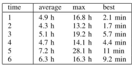
EXPERIMENTAL RESULTS FORc-AHP-M,2-AHC-M,ANDc-AHC-M
time average max best 1 4.9 h 16.8 h 2.1 min 2 4.3 h 13.2 h 1.7 min 3 5.1 h 19.2 h 5.7 min 4 4.7 h 14.1 h 4.4 min 5 7.2 h 28.1 h 11 min 6 6.3 h 16.3 h 9.2 min
In Table II, 1 – OA[3] forc-AHP-M with 3SAT reduction
γ[2] and random data from [33]; 2 – OA[3] for c -AHP-M with 3SAT reduction γ[2] and natural random data; 3 – OA[3] for 2-AHC-M with 3SAT reduction γ[3] and random data from [33]; 4 – OA[3] for2-AHC-M with 3SAT reduction γ[3] and natural random data; 5 – OA[3] for c -AHC-M with 3SAT reduction γ[4] and random data from [33]; 6 – OA[3] for c-AHC-M with 3SAT reduction γ[4]
and natural random data.
TABLE III
EXPERIMENTAL RESULTS FOR2-AHP-D,c-AHP-D,2-AHC-D,AND c-AHC-D
time average max best 1 19 min 2.3 h 57 sec 2 9 min 1.6 h 32 sec 3 1.3 h 4.7 h 1.9 min 4 1.1 h 3.4 h 1.1 min 5 2.2 h 5.3 h 3.8 min 6 1.9 h 3.9 h 2.4 min 7 4.3 h 21.4 h 6.3 min 8 3.8 h 9.7 h 4.8 min
In Table III, 1 – OA[3] for2-AHP-D with 3SAT reduction
3 – OA[3] for c-AHP-D with 3SAT reduction γ[2] and random data from [33]; 4 – OA[3] forc-AHP-D with 3SAT reduction γ[2] and natural random data; 5 – OA[3] for 2 -AHC-D with 3SAT reduction γ[3] and random data from [33]; 6 – OA[3] for2-AHC-D with 3SAT reductionγ[3]and natural random data; 7 – OA[3] for c-AHC-D with 3SAT reduction γ[4]and random data from [33]; 8 – OA[3] forc -AHC-D with 3SAT reductionγ[4]and natural random data.
VII. BENNETT’S MODEL OF CITOGENETICS
Regularities in a biological sequence can be used to identify important knowledge about the underlying biolog-ical system (see e.g. [35]–[37]). In particular, the study of genome rearrangements has drawn a lot of attention in recent years (see e.g. [38], [39]). According to Bennett’s model of cytogenetics (see e.g. [40]) the order in chromosome complements is based on a similarity relation which gives rise to a multigraphG. The multigraphGis the edge disjoint union of two of its subgraphs G1 and G2. We can assume
that the edges ofG1is the set of red edges and the edges of G2 is the set of blue edges. The order of the chromosomes
is determined by an alternating Hamiltonian path of G(see e.g. [40]).
We have designed generators of natural instances of 2 -AHP-M for Bennett’s model of cytogenetics. Selected ex-perimental results are given in the Table IV.
TABLE IV
EXPERIMENTAL RESULTS FORBENNETT’S MODEL OF CYTOGENETICS
time average max best 1 36 min 5.2 h 3.4 min 2 24.1 min 3.7 h 23 sec
In Table IV, 1 – OA[3] with 3SAT reduction γ[1]; 2 – OA[3] with 3SAT reductionγ[2]. It should be noted that in this caseγ[2]gives us significantly better performance.
VIII. AUTOMATIC GENERATION OF RECOGNITION MODULES
Usage of specialized modules of recognition gives us a significant advantage in solving concrete robotic and techni-cal vision tasks (see e.g. [41]–[43]). However, in this case, we need a large number of such modules. It is clear that we get a significant advantage if we use an automatic generation of such modules (see e.g. [44]). One of the main problems of automatic generation of recognition modules is a problem of study of new objects. In many self-learning systems, to solve this problem we need a training set which represents a set of configurations of the system and a set of confirmations and contradictions for the object (see e.g. [44], [45]). It is easy to see that such training set can be represented by some2 -edge-colored digraphD. In this case, to setup a self-learning process we need to solve2-AHP-D forD. We have designed a generator of natural instances for automatic generation of recognition modules. Selected experimental results are given in the Table V.
In Table V, 1 – OA[3] with 3SAT reduction γ[1]; 2 – OA[3] with 3SAT reduction γ[2].
TABLE V
EXPERIMENTAL RESULTS FOR AUTOMATIC GENERATION OF RECOGNITION MODULES
time average max best 1 31.4 min 7.5 h 2.9 min 2 54.6 min 11.1 h 19.3 min
IX. ROBOT SELF-AWARENESS
Robot self-awareness is an another area where we need to consider a set of configurations of the system and a set of confirmations and contradictions for the object. In particular, we have considered Occam’s razor model to anticipate collisions of the mobile robot with objects from the environment [46].
Using a model of on-line navigation in environments with dynamic obstacles, the robot needs to solve the question “Is it true that an obstacle 1 has continued behind an obstacle 2?” and to construct a local strategy of motion depending on the answer. To solve the question the robot can use some Occam’s razor model. Such model can be constructed by some genetic algorithm. Another genetic algorithm can be used to construct a local strategy of motion depending on the answer. Usage of two genetic algorithms requires some solution of the problem of their co-training. We use a sequential approach to learning. First, we train a genetic algorithm for Occam’s razor model. After this, we train a genetic algorithm for construction of a local strategy of motion depending on the answer.
It should be noted that quality of learning of a genetic algorithm for construction of a local strategy depends es-sentially on the distribution of obstacles (see Tables VI and VII).
TABLE VI
QUALITY OF PREDICTION OF A GENETIC ALGORITHM WITH DIFFERENT PROBABILITY OF ANSWER“YES”
number of p= 0.5 p= 0.3 p= 0.1 p= 0.7 p= 0.9 generations
0 43 % 37 % 49 % 38 % 47 %
10 44 % 39 % 50 % 39 % 48 %
102
46 % 41 % 53 % 40 % 49 %
103
55 % 42 % 54 % 41 % 50 %
104
71 % 47 % 55 % 45 % 52 %
105
94 % 56 % 56 % 55 % 53 %
106
97 % 68 % 59 % 63 % 57 %
In Table VI, we consider random distributions wherepis the probability of answer “yes”.
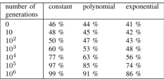
TABLE VII
QUALITY OF PREDICTION OF A GENETIC ALGORITHM WITH PROBABILITYp= 0.5OF ANSWER“YES”
number of constant polynomial exponential generations
0 46 % 44 % 41 %
10 48 % 45 % 42 %
102
50 % 47 % 43 %
103
60 % 53 % 48 %
104
77 % 63 % 56 %
105
97 % 85 % 74 %
106
99 % 91 % 86 %
In view of results of Tables VI and VII, it is of interest to consider2-AHP-D to generate a set of configurations of the system and a set of confirmations and contradictions for the object. Selected experimental results are given in the Table VIII.
TABLE VIII
THE DEPENDENCE OF THE NUMBER OF GENERATIONS AND QUALITY OF PREDICTION OF THE GENETIC ALGORITHM
0 10 102 103 104
44 % 47 % 58 % 83 % 96 %
X. ALGORITHMIC PROBLEMS IN ALGEBRA AND GRAPHS Many algorithmic problems of algebra are solved by in-vestigation of sequences of applications of defining relations. In particular, we can mention algorithmic problems of rings (see e.g. [47]–[50]), semigroups (see e.g. [51]–[55]), and groups (see e.g. [56]). Such sequences can be represented by different graph models.
There are a number of general connections between graphs and algorithmic problems in algebra. In particular, we can mention Cayley networks (see e.g. [39]), rewrite systems (see e.g. [57]), configuration graph for interpretations of Minsky machines (see e.g. [58]–[65]) and Turing machines (see e.g. [66]), etc. Note that in case of Minsky machines and Turing machines, traditional connections with graphs are slightly inconvenient. In Minsky machines and Turing machines, we consider directed transformations. In algebraic models, we consider undirected transformations. Therefore, it is natural to use H¨aggkvist transformation [13] and consider 2 -edge-colored multigraphs instead of traditional digraphs.
Using this approach we have created a test set based on the algebraic data. Selected experimental results are given in the Table IX.
TABLE IX
EXPERIMENTAL RESULTS FOR THE ALGEBRAIC DATA
time average max best 1 38.2 min 4.9 h 7.2 min 2 1.8 h 16.3 h 43.6 min
In Table IX, 1 – OA[3] with 3SAT reduction γ[1]; 2 – OA[3] with 3SAT reduction γ[2].
XI. THE PLANNING A TYPICAL WORKING DAY FOR INDOOR SERVICE ROBOTS PROBLEM
Different problems of planning and scheduling are among the most rapidly developing areas of modern computer science (see e.g. [67]–[71]). In particular, planning problems for mobile robots are of considerable interest for many years (see e.g. [11], [18], [22], [31], [72]–[81]). In [11], we have obtained an explicit reduction from the planning a typical working day for indoor service robots problem to HP-D. Also, in [11], we have used an explicit reduction [82] from HP-D to 3SAT. Note that we can use γ[1] and γ[2] to to create a solver for the planning a typical working day for indoor service robots problem and HP-D. We have designed generators of natural instances for the planning a typical working day for indoor service robots problem and HP-D. Selected experimental results are given in the Table X.
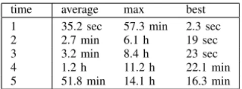
TABLE X
EXPERIMENTAL RESULTS FOR THE PLANNING A TYPICAL WORKING DAY FOR INDOOR SERVICE ROBOTS PROBLEM
time average max best 1 35.2 sec 57.3 min 2.3 sec 2 2.7 min 6.1 h 19 sec 3 3.2 min 8.4 h 23 sec 4 1.2 h 11.2 h 22.1 min 5 51.8 min 14.1 h 16.3 min
In Table X, 1 – OA[3] with 3SAT reduction γ[1]; 2 – OA[3] with 3SAT reduction γ[2]; 3 – OA[3] with 3SAT reduction [82]; 4 – fgrasp with 3SAT reduction [82]; 5 – posit with 3SAT reduction [82].
XII. THEHAMILTONIAN PATH PROBLEM
It is easy to see that we can use SAT solvers for2-AHP-M andc-AHP-M to solve HP-D. Selected experimental results are given in the Table XI.
TABLE XI
EXPERIMENTAL RESULTS FOR THEHAMILTONIAN PATH PROBLEM
time average max best 1 15.2 min 2.7 h 43 sec 2 26.1 min 5.4 h 8.4 min
In Table XI, 1 – OA[3] with 3SAT reduction γ[1]; 2 – OA[3] with 3SAT reductionγ[2].
XIII. CONCLUSION
In this paper we have considered an approach to create solvers for alternating Hamiltonian problems. In particular, explicit polynomial reductions from the decision versions of these problems to 3SAT is constructed. Also, we have considered computational experiments for alternating Hamil-tonian problems, Bennett’s model of cytogenetics, automatic generation of recognition modules, algebraic data, the plan-ning a typical working day for indoor service robots problem, and the Hamiltonian path problem.
REFERENCES
[1] A. Gorbenko and V. Popov, “Monochromatic s-t Paths in Edge-Colored Graphs,” Advanced Studies in Biology, vol. 4, no. 10, pp. 497-500, November 2012.
[2] A. Gorbenko and V. Popov, “The Hamiltonian Strictly Alternating Cycle Problem,”Advanced Studies in Biology, vol. 4, no. 10, pp. 491-495, November 2012.
[3] J. Bang-Jensen and G. Gutin, “Alternating cycles and paths in edge-coloured multigraphs: a survey,”Discrete Mathematics, vol. 165-166, no. 15, pp. 39-60, March 1997.
[4] J. Bang-Jensen and G. Gutin,Digraphs: Theory, Algorithms and Appli-cations. London, United Kingdom: Springer-Verlag, 2006. [5] D. Dorniger, “Hamiltonian circuits determining the order of
chromos-somes,”Discrete Applied Mathematics, vol. 50, no. 2, pp. 159-168, May 1994.
[6] P. Pevzner, “DNA physical mapping and properly edge-colored eurelian cycles in colored graphs,”Algorithmica, vol. 13, no. 1-2, pp. 77-105, February 1995.
[7] P. Pevzner, Computational Molecular Biology: An Algorithmic Ap-proach. Cambridge, Massachusetts, USA: MIT Press, 2000. [8] L. Gourv`es, A. Lyra, C. Martinhon, and J. Monnot, “The minimum
reload s-t path, trail and walk problems,”Discrete Applied Mathematics, vol. 158, no. 13, pp. 1404-1417, July 2010.
[10] T. C. Hu, Y. S. Kuo, “Graph folding and programmable logical arrays,”
Networks, vol. 17, no. 1, pp. 19-37, February 1987.
[11] A. Gorbenko, M. Mornev, and V. Popov, “Planning a Typical Working Day for Indoor Service Robots,” IAENG International Journal of Computer Science, vol. 38, no. 3, pp. 176-182, August 2011. [12] E. Bampis, Y. Manoussakis, and Y. Milis, “On the parallel complexity
of the alternating hamiltonian cycle problem,”RAIRO on Operations Research, vol. 33, no. 4, pp. 421-437, October 1999.
[13] Y. Manoussakis, “Alternating paths in edge-coloured complete graphs,”
Discrete Applied Mathematics, vol. 56, no. 2-3, pp. 297-309, January 1995.
[14] A. G. Chetwynd and A. J. W. Hilton, “Alternating Hamiltonian cycles in two colored complete bipartite graphs,”Journal of Graph Theory, vol. 16, no. 2, pp. 153-158, June 1992.
[15] M. R. Garey and D. S. Johnson,Computers and Intractability. A Guide to the Theory of NP-completeness. San Francisco, California, USA: W. H. Freeman and Co, 1979.
[16] A. Gorbenko, M. Mornev, V. Popov, and A. Sheka, “The problem of sensor placement for triangulation-based localisation,”International Journal of Automation and Control, vol. 5, no. 3, pp. 245-253, August 2011.
[17] A. Gorbenko and V. Popov, “The set of parameterized k-covers problem,”Theoretical Computer Science, vol. 423, no. 1, pp. 19-24, March 2012.
[18] A. Gorbenko and V. Popov, “Programming for Modular Reconfig-urable Robots,”Programming and Computer Software, vol. 38, no. 1, pp. 13-23, January 2012.
[19] A. Gorbenko, V. Popov, and A. Sheka, “Localization on Discrete Grid Graphs,” inProceedings of the CICA 2011, 2012, pp. 971-978. [20] A. Gorbenko and V. Popov, “The Longest Common Parameterized
Subsequence Problem,”Applied Mathematical Sciences, vol. 6, no. 58, pp. 2851-2855, March 2012.
[21] A. Gorbenko and V. Popov, “The Problem of Selection of a Minimal Set of Visual Landmarks,”Applied Mathematical Sciences, vol. 6, no. 95, pp. 4729-4732, October 2012.
[22] A. Gorbenko and V. Popov, “The Binary Paint Shop Problem,”Applied Mathematical Sciences, vol. 6, no. 95, pp. 4733-4735, October 2012. [23] A. Gorbenko and V. Popov, “The Longest Common Subsequence
Problem,”Advanced Studies in Biology, vol. 4, no. 8, pp. 373-380, June 2012.
[24] A. Gorbenko and V. Popov, “Element Duplication Centre Problem and Railroad Tracks Recognition,”Advanced Studies in Biology, vol. 4, no. 8, pp. 381-384, June 2012.
[25] A. Gorbenko, M. Mornev, V. Popov, and A. Sheka, “The Problem of Sensor Placement,”Advanced Studies in Theoretical Physics, vol. 6, no. 20, pp. 965-967, July 2012.
[26] A. Gorbenko and V. Popov, “On the Problem of Sensor Placement,”
Advanced Studies in Theoretical Physics, vol. 6, no. 23, pp. 1117-1120, November 2012.
[27] A. Gorbenko and V. Popov, “On the Longest Common Subsequence Problem,”Applied Mathematical Sciences, vol. 6, no. 116, pp. 5781-5787, November 2012.
[28] A. Gorbenko and V. Popov, “The c-Fragment Longest Arc-Preserving Common Subsequence Problem,”IAENG International Journal of Com-puter Science, vol. 39, no. 3, pp. 231-238, August 2012.
[29] A. Gorbenko and V. Popov, “Computational Experiments for the Problem of Selection of a Minimal Set of Visual Landmarks,”Applied Mathematical Sciences, vol. 6, no. 116, pp. 5775-5780, November 2012. [30] A. Gorbenko and V. Popov, “On the Problem of Placement of Visual Landmarks,”Applied Mathematical Sciences, vol. 6, no. 14, pp. 689-696, January 2012.
[31] A. Gorbenko and V. Popov, “On the Optimal Reconfiguration Plan-ning for Modular Self-Reconfigurable DNA Nanomechanical Robots,”
Advanced Studies in Biology, vol. 4, no. 2, pp. 95-101, March 2012. [32] A. Gorbenko and V. Popov, “Task-resource Scheduling Problem,”
International Journal of Automation and Computing, vol. 9, no. 4, pp. 429-441, August 2012.
[33] SATLIB — The Satisfiability Library. [Online]. Available: http://people.cs.ubc.ca/∼hoos/SATLIB/index-ubc.html
[34] Web page “Computational resources of IMM UB RAS”. (In Russian.) [Online]. Available:
http://parallel.imm.uran.ru/mvc now/hardware/supercomp.htm [35] V. Popov, “The approximate period problem for DNA alphabet,”
Theoretical Computer Science, vol. 304, no. 1-3, pp. 443-447, July 2003.
[36] V. Popov, “The Approximate Period Problem,”IAENG International Journal of Computer Science, vol. 36, no. 4, IJCS 36 4 03, November 2009.
[37] V. Yu. Popov, “Computational complexity of problems related to DNA sequencing by hybridization,”Doklady Mathematics, vol. 72, no. 1, pp. 642-644, July-August 2005.
[38] V. Popov, “Multiple genome rearrangement by swaps and by element duplications,”Theoretical Computer Science, vol. 385, no. 1-3, pp. 115-126, October 2007.
[39] V. Popov, “Sorting by prefix reversals,”IAENG International Journal of Applied Mathematics, vol. 40, no. 4, IJAM 40 4 02, November 2010.
[40] D. Dorninger, “Hamiltonian circuits determining the order of chro-mosomes,”Discrete Applied Mathematics, vol. 50, no. 2, pp. 159-168, May 1994.
[41] A. Gorbenko and V. Popov, “On Face Detection from Compressed Video Streams,” Applied Mathematical Sciences, vol. 6, no. 96, pp. 4763-4766, October 2012.
[42] A. Gorbenko and V. Popov, “Usage of the Laplace Transform as a Basic Algorithm of Railroad Tracks Recognition,”International Journal of Mathematical Analysis, vol. 6, no. 48, pp. 2413-2417, October 2012. [43] A. Gorbenko and V. Popov, “A Real-World Experiments Setup for Investigations of the Problem of Visual Landmarks Selection for Mobile Robots,”Applied Mathematical Sciences, vol. 6, no. 96, pp. 4767-4771, October 2012.
[44] A. Gorbenko and V. Popov, “Self-Learning Algorithm for Vi-sual Recognition and Object Categorization for Autonomous Mobile Robots,” inProceedings of the CICA 2011, 2012, pp. 1289-1295. [45] A. Gorbenko, A. Lutov, M. Mornev, and V. Popov, “Algebras of
Stepping Motor Programs,”Applied Mathematical Sciences, vol. 5, no. 34, pp. 1679-1692, June 2011.
[46] A. Gorbenko and V. Popov, “Anticipation in Simple Robot Navigation and Learning of Effects of Robot’s Actions and Changes of the Environment,”International Journal of Mathematical Analysis, vol. 6, no. 55, pp. 2747-2751, November 2012.
[47] V. Yu. Popov, “Critical theories of supervarieties of the variety of commutative associative rings,”Siberian Mathematical Journal, vol. 36, no. 6, pp. 1184-1193, November 1995.
[48] V. Yu. Popov, “Critical theories of varieties of nilpotent rings,”Siberian Mathematical Journal, vol. 38, no. 1, pp. 155-164, January 1997. [49] V. Yu. Popov, “A ring variety without an independent basis,”
Mathe-matical Notes, vol. 69, no. 5-6, pp. 657-673, May 2001.
[50] Yu. M. Vazhenin and V. Yu. Popov, “On positive and critical theories of some classes of rings,”Siberian Mathematical Journal, vol. 41, no. 2, pp. 224-228, April 2000.
[51] V. Yu. Popov, “On connection between the word problem and decid-ability of the equational theory,”Siberian Mathematical Journal, vol. 41, no. 5, pp. 921-923, September 2000.
[52] V. Yu. Popov, “Critical theories of varieties of semigroups satisfying a permutation identity,”Siberian Mathematical Journal, vol. 42, no. 1, pp. 134-136, January 2001.
[53] V. Yu. Popov, “On the finite base property for semigroup varieties,”
Siberian Mathematical Journal, vol. 43, no. 5, pp. 910-919, September 2002.
[54] V. Yu. Popov, “Markov properties of burnside varieties of semigroups,”
Algebra and Logic, vol. 42, no. 1, pp. 54-60, January 2003.
[55] V. Yu. Popov, “The property of having independent basis in semigroup varieties,”Algebra and Logic, vol. 44, no. 1, pp. 46-54, January 2005. [56] Yu. M. Vazhenin and V. Yu. Popov, “Decidability boundaries for some classes of nilpotent and solvable groups,”Algebra and Logic, vol. 39, no. 2, pp. 73-77, January 2000.
[57] O. G. Kharlampovich and M. V. Sapir, “Algorithmic problems in varieties,”International Journal of Algebra and Computation, vol. 5, no. 4-5, pp. 379-602, August-October 1995.
[58] V. Yu. Popov, “On the decidability of equational theories of varieties of rings,”Mathematical Notes, vol. 63, no. 6, pp. 770-776, June 1998. [59] V. Yu. Popov, “On equational theories of varieties of anticommutative rings,”Mathematical Notes, vol. 65, no. 2, pp. 188-201, February 1999. [60] V. Yu. Popov, “On the derivable identity problem in varieties of rings,”
Siberian Mathematical Journal, vol. 40, no. 5, pp. 948-953, October 1999.
[61] V. Yu. Popov, “On equational theories of classes of finite rings,”
Siberian Mathematical Journal, vol. 40, no. 3, pp. 556-564, May 1999. [62] V. Yu. Popov, “Undecidability of the word problem in relatively free rings,”Mathematical Notes, vol. 67, no. 4, pp. 495-504, April 2000. [63] V. Yu. Popov, “Equational theories for classes of finite semigroups,”
Algebra and Logic, vol. 40, no. 1, pp. 55-66, January 2001.
[64] V. Yu. Popov, “Decidability of equational theories of coverings of semigroup varieties,”Siberian Mathematical Journal, vol. 42, no. 6, pp. 1132-1141, November 2001.
[65] V. Popov, “The word problem for relatively free semigroups,” Semi-group Forum, vol. 72, no. 1, pp. 1-14, February 2006.
[67] P. Bertoli, M. Pistore, and P. Traverso, “Automated composition of Web services via planning in asynchronous domains,”Artificial Intelligence, vol. 174, no. 3-4, pp. 316-361, March 2010.
[68] S. Srivastava, N. Immerman, and S. Zilberstein, “A new representation and associated algorithms for generalized planning,”Artificial Intelli-gence, vol. 175, no. 2, pp. 615-647, February 2011.
[69] K. Wang and S. H. Choi, “Decomposition-Based Scheduling for Makespan Minimisation of Flexible Flow Shop with Stochastic Process-ing Times,”Engineering Letters, vol. 18, no. 1, EL 18 1 09, February 2010.
[70] F. Wu, S. Zilberstein, and X. Chen, “Online planning for multi-agent systems with bounded communication,”Artificial Intelligence, vol. 175, no. 2, pp. 487-511, February 2011.
[71] M. Zhongyi, M. Younus, and L. Yongjin, “Automated Planning and Scheduling System for the Composite Component Manufacturing Work-shop,”Engineering Letters, vol. 19, no. 1, pp. 75-83, February 2011. [72] A. Boonkleaw, N. Suthikarnnarunai, and R. Srinon, “Strategic
Plan-ning for Newspaper Delivery Problem Using Vehicle Routing Algorithm with Time Window (VRPTW),”Engineering Letters, vol. 18, no. 2, EL 18 2 09, May 2010.
[73] J.-W. Choi, R. E. Curry, and G. H. Elkaim, “Continuous Curvature Path Generation Based on Bezier Curves for Autonomous Vehicles,”
IAENG International Journal of Applied Mathematics, vol. 40, no. 2, IJAM 40 2 07, May 2010.
[74] G. B. Dantzig and J. H. Ramser, “The Truck Dispatching Problem,”
Management Science, vol. 6, no. 1, pp. 80-91, October 1959. [75] A. Gorbenko and V. Popov, “Robot Self-Awareness: Occam’s Razor
for Fluents,”International Journal of Mathematical Analysis, vol. 6, no. 30, pp. 1453-1455, March 2012.
[76] A. Gorbenko and V. Popov, “The Force Law Design of Artificial Physics Optimization for Robot Anticipation of Motion,” Advanced Studies in Theoretical Physics, vol. 6, no. 13, pp. 625-628, March 2012. [77] A. Gorbenko, V. Popov, and A. Sheka, “Robot Self-Awareness: Ex-ploration of Internal States,”Applied Mathematical Sciences, vol. 6, no. 14, pp. 675-688, January 2012.
[78] A. Gorbenko, V. Popov, and A. Sheka, “Robot Self-Awareness: Tem-poral Relation Based Data Mining,”Engineering Letters, vol. 19, no. 3, pp. 169-178, August 2011.
[79] P. Sotiropoulos, N. Aspragathos, and F. Andritsos, “Optimum Docking of an Unmanned Underwater Vehicle for High Dexterity Manipulation,”
IAENG International Journal of Computer Science, vol. 38, no. 1, pp. 48-56, February 2011.
[80] M. Sridharan, J. Wyatt, R. Dearden, “Planning to see: A hierarchical approach to planning visual actions on a robot using POMDPs,”
Artificial Intelligence, vol. 174, no. 11, pp. 704-725, July 2010. [81] X. Zheng, S. Koenig, D. Kempe, and S. Jain, “Multi-Robot Forest
Coverage for Weighted and Unweighted Terrain,”IEEE Transactions on Robotics, vol. 26, no. 6, pp. 1018-1031, November 2010. [82] K. Iwama and S. Miyazaki, “SAR-variable complexity of hard
com-binatorial problems,” inInformation Processing 94, IFIP Transactions A, Computer Science and Technology, vol. I, pp. 253-258.
Anna Gorbenkowas born on December 28, 1987. She received her M.Sc. in Computer Science from Department of Mathematics and Mechanics of Ural State University in 2011. She is currently a graduate student at Mathematics and Computer Science Institute of Ural Federal University and a researcher at Department of Intelligent Sys-tems and Robotics of Mathematics and Computer Science Institute of Ural Federal University. She has (co-)authored 2 books and 18 papers. She has received Microsoft Best Paper Award from international conference in 2011.