ISSN 0101-8205 / ISSN 1807-0302 (Online) www.scielo.br/cam
An alternating LHSS preconditioner
for saddle point problems
LIU QINGBING1,2∗
1Department of Mathematics, Zhejiang Wanli University, Ningbo, Zhejiang, 315100, P.R. China 2Department of Mathematics, East China Normal University, Shanghai, 200241, P.R. China
E-mail: [email protected]
Abstract. In this paper, we present a new alternating local Hermitian and skew-Hermitian splitting preconditioner for solving saddle point problems. The spectral property of the precondi-tioned matrices is studies in detail. Theoretical results show all eigenvalues of the precondiprecondi-tioned matrices will generate two tight clusters, one is near(0,0)and the other is near(2,0)as the iteration parameter tends to zero from positive. Numerical experiments are given to validate the performances of the preconditioner.
Mathematical subject classification: Primary: 65F10; Secondary: 65F50.
Key words:saddle point problems, matrix splitting, preconditioner, eigenvalue distribution.
1 Introduction
We study a new preconditioner for saddle point systems of the type
Au =
"
A BT −B 0
# "
x y
#
=
"
f g
#
=b, (1)
whereA ∈ Rn×nis a positive real matrix, that is, the matrix H =(A+AT)/2,
the symmetric part ofA, is positive definite,B∈ Rm×nwithm ≤nhas full row
rank. Such linear systems arise in a large number of scientific and engineering
#CAM-376/11. Received: 30/V/11. Accepted: 26/VII/11.
∗Author supported by National Natural Science Foundation of China (No. 11071079) and
applications (see for instance [6, 13, 17]). As such systems are typically large and sparse, solution by iterative methods can be found in the literature, such as Uzawa-type schemes [6], splitting methods [2, 3, 15], iterative projection methods [17], iterative null space methods [6, 17] etc. To improve the conver-gence of rate of iterative methods, preconditioning techniques have been studied and many effective preconditioners have been employed for solving linear sys-tems of the form (1) [2-8, 11-14, 16, 18].
Recently, based on the Hermitian and skew-Hermitian splitting of the saddle point matrix, a general alternating preconditioner for generalized saddle point problems was analyzed in [5]. Bai et al. [1] further generalized HSS to positive-definite and skew-Hermitian splitting (PSS), Normal and skew-Hermitian split-ting (NSS) and considered preconditioners based on the splitsplit-ting. Pan et al. [14] proposed two preconditioners for the saddle point problem (1), using the HS splitting and PS splitting of the (1,1) blocks A, not based on use of the coef-ficient matrixAas a preconditioner for Krylov subspace methods. Peng and Li [15] considered a kind of the alternating-direction iterative method which is based on the block triangular splitting of the coefficient matrix, and its precon-ditioned version was established in [16]. In [16], the alternating preconditioner was further studied as a preconditioner of some Krylov subspace methods for the saddle point problems.
In this paper, we propose a new alternating local Hermitian and skew-Hermitian splitting preconditioner for the saddle point problem (1) based on the HS split-ting of the (1,1) blocks A. We mainly focus on the case that Ais positive real matrix with the symmetric part. We first establish a new alternating-direction iterative method for the saddle point problem (1) and then give a new alternating local Hermitian and skew-Hermitian splitting preconditioner in Section 2, and spectral properties of the preconditioned matrix are discussed in detail. Numer-ical experiments are presented in Section. In the final section, we draw some conclusions.
2 The new preconditioner and its spectral properties From now on, we will adopt the general notation
A=
"
A BT −B 0
#
to represent the nonsymmetric saddle point matrix of equation (1). We assume thatAis positive real, and that Bis of sizem×nand has full row rank.
LetA=Hf+Se, where
f
H =
"
H BT
0 0
#
and eS=
"
S 0
−B 0
#
with
H = 1
2(A+A
T
) and S = 1
2(A−A
T
).
2.1 The preconditioner
Analogously to the classical ADI method [19], we consider the following two splittings ofA:
A=(αI +Hf)−(αI −eS)=(αI +eS)−(αI −Hf)
whereα >0 is a parameter andI is the identity matrix. By iterating alternatively between this two splittings, we obtain a new algorithm as follows:
(αI +Hf)uk+12
=(αI −Se)uk,
(αI +Se)uk+1=(αI −Hf)uk+12,
k =0,1,2, . . . , (3)
whereu0 is an initial guess. By eliminating the intermediate vectoruk+12, we
have the iteration in fixed point form as
uk+1=Tαuk +c,
where
Tα =(αI +Se)−1
(αI −Hf)(αI +Hf)−1
(αI −eS),
and
c =(αI +eS)−1
[I +(αI −Hf)(αI +Hf)−1
]b.
It is easy to know that there is a unique splitting A = Pα −Nα, with Pα nonsingular, which induces the iteration matrixTα, i.e.,
Tα =P−1
where
Pα = 1
2α(αI +Hf)(αI +eS).
Hence, the linear systemAu =bis equivalent to the linear system (I −P−1
α Nα)u=Pα−1Au=c.
Recently, for generalized linear systems, the estimates for the spectral radius ofρ(P−1
α A)with the HSS preconditionerPα with H = A have been studied
in [16]. However, if we use a Krylov subspace method such as GMRES or its restarted variant to approximate the solution of this system of linear equations, Pα can be considered as a new preconditioner to the saddle point problems (1). Under the assumption that A is positive real, analogously to the proof in [11] we can show that all eigenvalues of the preconditioned matrices will generate two tight clusters, one is near(0,0)and the other is near(2,0)as the iteration parameter tends to zero from positive.
2.2 Spectral properties
It is well known that characterizing the rate of convergence of nonsymmetric pre-conditioned iterations can be a difficult task. In particular, eigenvalue informa-tion alone may not be sufficient to give meaningful estimates of the convergence rate of a method like preconditioned GMRES [6, 17]. Nevertheless, experi-ence shows that for many linear systems arising in practice, a well-clustered spectrum (away from zero) usually results in rapid convergence of the precon-ditioned iteration. Now we consider the eigenvalue problem associated with the preconditioned matrixρ(P−1
α A), i.e.,
Ax =λPαx, (4)
where(λ,x)is any eigenpair ofρ(P−1
α A). It is easy to know thatλ6= 0 from
Anonsingular. Then we have
"
A BT
−B 0
# " u v # = λ 2α "
αIn+H BT
0 αIm
# "
αIn+S 0 −B αIm
# "
f g
#
,
which leads to
2α(Au+BTv)=λ[(α2I +αA+H S)u+αBTv], (5)
First of all, it must holdu6=0. Otherwise, it follows from (6) that eitherλ=0 orv =0 holds. In fact, neither of them can be true.
Ifv=0, then from (5) we have 2αAu =λ(α2u+αAu+H Su). Multiplying both sides of this equality from left withu∗, we have
λ= 2αu
∗Au
α2u∗u+αu∗Au+u∗H Su. (7)
If u∗H Su = 0, from (7), it is easy to see that λ → 2 as α → 0+. If u∗H Su6=0, from (7), we have thatλ→0 asα →0
+.
We now assumev 6=0, without loss of generality, we further assumekvk =1 and substitute (6) to (5), we obtain
(−λ2+4λ−4)αB Au−(λ2−2λ)B H Su
−(λ2−4λ+4)αB BTv−λ2α3v =0. Multiplying the above equality from left hand byv∗, we obtain
(−αv∗B Au−v∗B H Su−αv∗B BTv−α3)λ2+(4αv∗B Au
+2v∗B H Su+4αv∗B BTv)λ−(4αv∗B Au+4αv∗B BTv)=0 (8)
Let
b1=v∗B Au+v∗B BTv, b2=v∗B H Su Then (8) can be rewritten as
−(αb1+b2+α3)λ2+(4αb1+2b2)λ−4αb1=0. (9) For simplicity, we denote thatδ=αb1+b2+α3. Subsequently, we will mainly discuss the two cases, that is to say,δ=0 andδ 6=0.
Case I. δ=0.
It is not difficult to know that 4αb1+2b2 6=0 from the existence eigenvalue of the preconditioned matrix. From (9), we have
λ= 2αb1
2αb1+b2
Sinceδ=αb1+b2+α3=0, we have
2αb1+b2=αb1−α3. (11) Substituting (11) to (10), we have
λ= 2b1
b1−α2
. (12)
Ifb1 = 0, from (12), it is easy to know that λ = 0. Ifb1 6= 0, we have that λ→2 asα→0+.
Case II. δ6=0. Note that
4(2αb1+b2)2−16αb1(αb1+b2+α3)=4(b22−4α 4
b1), then the two roots of the quadratic equation (9) are
λ±=
(2αb1+b2)±
q
b22−4α4b 1 αb1+b2+α3
.
We will mainly discuss in the following two cases:
1) Ifb2=0, then we have
λ±=
2b1±
p
−4α4b 1 b1+α2
.
1.1) Ifb1=0, then we have thatλ±=0.
1.2) Ifb16=0, then we have thatλ→2 asα→0+.
2) Ifb26=0, then we have
λ±→ b2±
q
b22 b2
=0 or 2 as α→0+.
Up to now, we have shown that the eigenvalues of the preconditioned matrix ρ(P−1
α A) will converge to either the origin or the point (2,0) as α → 0+.
matrixρ(P−1
α A)will gather into two cluster, one is near(0,0)and another is
near(2,0).
From the above discussing, we have the following theorem.
Theorem 2.1. LetAbe positive real and B has full row rank. x =(u∗, v∗)∗ is an eigenvector ofP−1
α A, then for sufficiently smallα > 0, the eigenvalue of
P−1
α Ahave the following cases:
(I) Ifv=0, then the eigenvalue ofP−1
α Awill gather into(0,0)or(2,0)as
α→0+.
(II) Ifv 6=0, then the eigenvalue ofP−1
α Awill gather into two clusters, one
is near(0,0)and another is near(2,0)asα →0+.
3 Numerical experiments
In this section, we present our numerical experiments to illustrate the eigenvalue distribution of the preconditioned matrixP−1
α Aand to assess our statement that
the eigenvalues ofP−1
α Awill be gathering into two clusters asαbecomes small.
We consider the saddle point-type matrixAof the following form:
A=
"
A BT
−B 0
#
(13)
where the sub-matricesA=υA1+N,Nhas only two diagonal lines of nonzero, which start from the 2nd and thenth colomns, i.e.,
N =
0 −1 0 ∙ ∙ ∙ 0 −1 0 ∙ ∙ ∙ 0
0 0 −1 ∙ ∙ ∙ 0 0 −1 . .. 0
0 0 0 −1 0 ∙ ∙ ∙ 0 . .. 0 ..
. . .. ... ... ... ... ∙ ∙ ∙ . .. −1 0 ∙ ∙ ∙ 0 0 0 −1 0 ∙ ∙ ∙ 0
0 0 ∙ ∙ ∙ 0 0 0 −1 0 ...
0 0 0 ∙ ∙ ∙ 0 0 0 −1 0
..
. . .. ... ... 0 . .. 0 . .. −1 0 ∙ ∙ ∙ 0 0 0 ∙ ∙ ∙ 0 0 0
andA1,Bare taken from [2], i.e.,
A1=
"
I ⊗T +T ⊗I 0 0 I ⊗T +T ⊗I
#
,B=
"
I ⊗F F⊗I
#
and
T = 1
h2tr i di ag(−1,2,−1)∈ R
p×p,F = 1
htr i di ag(−1,1,0)∈ R
p×p
with⊗being the Kronecker product symbol and h = 1
h+1 the discretization meshsize. The right vectors are defined as
f =(1,1,∙ ∙ ∙,1)∈ Rn,g=(0,0,∙ ∙ ∙ ,0)∈ Rm,n=2p2,m= p2. For this example, the matrix Ais nonsymmetric and positive real.
Theorem 1 shows that the eigenvalue ofP−1
α Awill gather into two clusters,
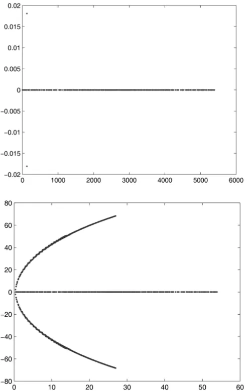
one is near(0,0)and another is near(2,0)asα→0+. We plot the spectra of the
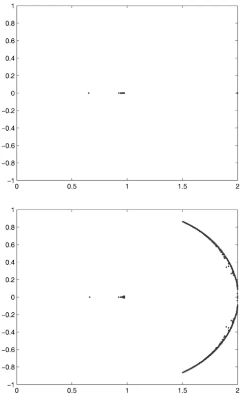
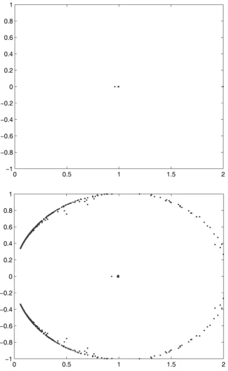
coefficient matrix withν=1 andν=0.01 from left column to right column in Figure 1, and the spectra of the preconditioned matrices corresponding toν=1 and different values ofα in Figures 2-4, where the left column corresponding to the preconditionerPcα and the right column corresponding to the precondi-tionerPα. From Figures 2-4 we can see that the eigenvalues of both kinds of preconditioned matrices become more and more clustered asαbecomes smaller. All the numerical experiments were performed with MATLAB 7.0. The ma-chine we have used is a PC-AMD, CPU T7400 2.2GHz process. The GMRES method is used to solve the above test problem. The initial guess is taken to be x(0)=0 and the stopping criterion is chosen as
kb−Ax(k)k
2
kbk2
≤10−6.
In Tables 1-2, we list the iteration numbers of GMRES and the preconditioned GMRES when they are applied to solve the test problem, where the numbers outside (inside) of the brackets denote outer iteration numbers (inner iteration numbers) of GMRES method, respectively.
Figure 1 – Eigenvalue distributions of the matrixAforν =1 andv=0.01.
preconditioner in [16] which is defined as follows:
c
Pα = 1
2α(αI +Hc)(αI +bS) with
c
H =
"
A BT
0 0
#
and Sb=
"
0 0
−B 0
Figure 2 – Spectrum of the preconditioned matrix with respect toPcαandPαasα=1.
Figure 3 – Spectrum of the preconditioned matrix with respect toPcαandPαasα=0.1.
Figure 4 – Spectrum of the preconditioned matrix with respect toPcαandPαasα=0.01.
4 Conclusions
m+n 768 1200 1587 1875 2700
GMRES(Pα) 9(7) 9(7) 7(6) 7(6) 7(7)
GMRES(Pcα) 4(8) 5(7) 5(10) 5(10) 5(10)
Table 1 – Iteration numbers for the test problem withν=1.
α 1.0 0.8 0.6 0.3 0.1
GMRES(Pα) 3(7) 4(2) 4(4) 5(10) 7(6)
GMRES(Pcα) 3(4) 3(9) 3(8) 4(8) 5(10)
Table 2 – Iteration numbers for the test problem withν=1 for differentα.
preconditioned linear systemP−1
α Ax=P −1
α brequires the solution of an inner
linear system whose coefficient matrix is Pα. Therefore, convergence of the outer iteration is fast if the eigenvalues of the preconditioned matrixP−1
α Aare
clustered, but careful attention must be paid to the conditioning and eigenvalue distribution of the matrixPα itself, which determine the speed of convergence of the inner iteration [10]. Therefore, how to reduce the outer and inner iteration numbers for such problems remains an extensive discussion.
Acknowledgments. The author is grateful to the anonymous referees for their helpful suggestions which improve this paper.
REFERENCES
[1] Z.Z. Bai, G.H. Golub and M.K. Ng, Hermitian and skew-Hermitian splitting methods for non-Hermitian positive definite linear systems. SIAM J. Matrix Anal. Appl.,24(2003), 603–626.
[2] Z.Z. Bai, G.H. Golub and J.Y. Pan, Preconditioned Hermitian and skew-Her-mitian splitting methods for non-Herskew-Her-mitian positive semidefinite linear systems. Numer. Math.,98(2004), 1–32.
[3] Z.Z. Bai, G.H. Golub, L.L. Zhang and J.F. Yin, Block triangular and skew-Her-mitian splitting methods for positive-definite linear systems. SIAM J. Sci. Comput., 26(2005), 844–863.
[4] Z.Z. Bai, M.K. Ng and Z.Q.Wang, Constraint preconditioners for symmetric indefinite matrices. SIAM J. Matrix Anal. Appl.,31(2009), 410–433.
[6] M. Benzi, G.H. Golub and J. Liesen, Numerical solution of saddle point problems. Acta Numerica.,14(2005), 1–137.
[7] M. Benzi and J. Liu, Block preconditioning for saddle point systems with indefinite
(1,1)block. Int. J. Comput. Math.,84(2007), 1117–1129.
[8] Z.H. Cao, Augmentation block preconditioners for saddle point-type matrices with singular(1,1)blocks. Numer. Linear Algebra Appl.,15(2008), 515–533.
[9] G.H. Golub and C. Greif, On solving block-structured indefinite linear systems. SIAM J. Sci. Comput.,24(2003), 2076–2092.
[10] C. Greif and M.L. Overton, An Analysis of Low-Rank Modifications of
Precon-ditioners for Saddle Point Systems. Electron. Trans. Numer. Anal., 37 (2010),
307–320.
[11] T.Z. Huang, S.L. Wu and C.X. Li, The spectral properties of the Hermitian and skew-Hermitian splitting preconditioner for generalized saddle point problems. J. Comput. Appl. Math.,229(2009), 37–46.
[12] H.S.Dollar and A.J. Wathen,Approximate factorization constraint precondition-ers for saddle point matrices. SIAM J. Sci. Comput.,27(2006), 1555–1572.
[13] H.C. Elman, D.J. Silvester and A.J. Wathen, Performance and analysis of saddle point preconditioners for the discrete stead-state Navier-Stokes equations. Numer. Math.,90(2002), 665–688.
[14] J.Y. Pan, M.K. Ng and Z.Z. Bai,New preconditioners for saddle point problems. Appl. Math. Comput.,172(2006), 762–771.
[15] X.F. Peng and W. Li, The alternating-direction iterative method for saddle point
problems. Appl. Math. Comput.,216(2010), 1845–1858.
[16] X.F. Peng and W. Li, An alternating preconditioner for saddle point problems. Appl. Math. Comput.,234(2010), 3411–3423.
[17] Y. Saad, Iterative Methods for Sparse Linear Systems. SIAM, Philadelphia, PA (2003).
[18] V. Simoncini,Block triangular preconditioners for symmetric saddle-point prob-lems. Appl. Numer. Math.,49(2004), 63–80.
[19] D.W. Peaceman and J.H.H. Rachford, The numerical solution of parabolic and elliptic differential equations. Journal of the Society for Industrial and Applied Mathematics,3(1955), 28–41.