Analytical functions for the calculation of hyperspherical potential curves of atomic systems

Analytical functions for the calculation of hyperspherical potential curves of atomic systems

J. J. De Groote,1Mauro Masili,2and J. E. Hornos3 1

Instituto de Quı´mica de Araraquara, Universidade Estadual Paulista, Caixa Postal 355, 14 801-970 Araraquara, SP, Brazil 2_{Department of Physics and Astronomy, The University of Nebraska, 116 Brace Laboratory, Lincoln, Nebraska 68 588-0111}

3_{Instituto de Fı´sica de Sa˜o Carlos, Universidade de Sa˜o Paulo, Caixa Postal 369, 13 560-970 Sa˜o Carlos, SP, Brazil}

~Received 8 March 2000; revised manuscript received 25 April 2000; published 15 August 2000!

We present angular basis functions for the Schro¨dinger equation of two-electron systems in hyperspherical coordinates. By using the hyperspherical adiabatic approach, the wave functions of two-electron systems are expanded in analytical functions, which generalizes the Jacobi polynomials. We show that these functions, obtained by selecting the diagonal terms of the angular equation, allow efficient diagonalization of the Hamil-tonian for all values of the hyperspherical radius. The method is applied to the determination of the 1_Se_energy

levels of the Li1_{and we show that the precision can be improved in a systematic and controllable way.}

PACS number~s!: 31.25.2v, 31.15.Ja, 31.15.Ar

I. INTRODUCTION

Hyperspherical coordinates have been used, for a long time, to solve the N-body quantum problems in molecular @1–5#, atomic @6–11#, and nuclear physics @12–14#. The standard approach begins with the introduction of Jacobi variables to eliminate the center-of-mass coordinates. The remaining 3N23 degrees of freedom are described by a ~hyper-! radius R and 3N24 angular variables V 5(v1, . . . ,v3N24) composed by N22 hyperspherical an-gular variables and by the 2N22 usual spherical angular variables ui and fi. The nonrelativistic kinetic-energy

op-erator is separable on those variables and its angular part can be identified with the Casimir operator of the O(3N23) symmetry group. The problem of constructing angular basis functions, which diagonalize the kinetic operator, is reduced to the well-established problem of construction of harmonic functions for the orthogonal groups. The irreducible repre-sentations of these groups can be labeled by a setl of inte-ger indices, and angular functions can be constructed using Jacobi polynomials for each representation.

In concrete applications, the attention is focused on the properties of the wave functions; however, the procedure is a part of the so-called algebraic methods@13#, in which a sym-metry group G is decomposed in a chain of subgroups G.G1.• • •.O(3) ending in the tridimensional rotation

group. The multidimensional orthogonal symmetry is bro-ken, not spontaneously by its subgroups but by the interpar-ticle interactions. The effects on the calculation will be the lack of convergence in the expansion by harmonic functions and the need of a large basis to reproduce the wave func-tions. The intensity of this effect will depend on how ‘‘badly’’ the symmetry was broken. The Coulombic three-body systems are an illustrative example on this process for which we usually choose the O(6).O(3)3O(3).O(3) chain. The O(3)3O(3) symmetry is lightly broken, leading to a reasonable convergence in the composed angular mo-mentum function, which characterizes this subgroup. In op-position, the O(6) symmetry is strongly broken due to the long range of the electromagnetic interaction. A much more favorable situation occurs in the nuclear problem, for which the short-range forces confine the particles, enhancing the

role of the kinetic terms. As a result, calculations of the wave function for nuclei with a mass number between two and ten have been reported @12#. In the atomic counterpart, the ap-plications are mainly limited to the three- and four-body case.

An alternative approach to the use of the multidimen-sional orthogonal basis is to solve the partial differential equation for the angular variables directly by expanding the angular function in a power series in appropriated variables @7#. The functions will not be eigenstates of the orthogonal group but will fully incorporate the interparticle interactions. This approach has been used in calculations of potential curves for helium, H2, D₂1, DDm, excitons and other spe-cies @2,15,16#. The inclusion of nonadiabatic couplings has been reported and accurate ground-state @17# and excited-state @18#energies were obtained.

The generalization of the hyperspherical adiabatic ap-proach~HAA!to complex atoms will require the solution of an infinite set of partial equations instead of ordinary equa-tions as in the three-body case, which is unpractical even in the lithium case. With this in mind, we reviewed the HAA, searching for a basis that can be used as building blocks for atomic and molecular calculations. The set of functions de-pends parametrically on the hyperspherical radius R. At the R50 limit, they reproduce the Jacobi polynomials and at the R→` limit, the Laguerre functions behavior, which charac-terizes the Coulombic problem, is exactly achieved. The functions are obtained extracting the diagonal part of the interactions for all angular momentum manifolds. The func-tions are transcendental but their Taylor expansion coeffi-cients can be calculated with arbitrary precision.

In order to verify the efficiency of our procedure, we ana-lyze the potential curves and nonadiabatic couplings for Li1

and compare the corresponding lowest energies with values obtained by other methods. We observed that the curves have been calculated accurately and the long-range problems are absent.

present the solutions of the method for the Li1 _{ion and}

fi-nally, Sec. V is dedicated to the conclusion.

II. HYPERSPHERICAL ADIABATIC APPROACH

The HAA is an adequate method to treat N-body systems interacting with the long-range Coulombian forces due to its molecularlike description that brings to mind the spirit of the Born-Oppenheimer approximation. With the choice of ap-propriate Jacobi coordinates, the center-of-mass degrees of freedom can be excluded and the hyperspherical coordinates are built in order to correlate the remaining N21 radial co-ordinates. Those coordinates are composed to bring about only one radial component R,

R25

(

i51

N21 ri

2

~0<R<` !, ~1!

and also angular variables that can be related to the Jacobi radial coordinates rW1,rW2, . . . ,rWN21 as @12#

r₁5R sin~aN22!• • •sin~a2!sin~a1!,

r25R sin~aN22!• • •sin~a2!cos~a1!,

r₃5R sin~aN22!• • •cos~a2!,

A

r_N225R sin~aN22!cos~aN23!,

rN215R cos~aN22! ~0<ai<p/2!. ~2!

With those coordinates, the hyperspherical Schro¨dinger equation has the compact form

F

d2

dR21

~3N24!

R d

dR1

Uˆ~R;V !

R2 12«

G

c~R,V !50, ~3!

where« is the system energy and the operator Uˆ (R;V) de-pends on all compact variables V5(ai,fj,uj;i51, . . . ,N 22; j51, . . . ,N21) and on the hyperradius R through the expression

Uˆ5C2@O~3N23!#1RVˆ~R;V !, ~4!

where C2 is the Casimir operator of the O(3N23) group and Vˆ /R is the interparticle potential energy. In the case of Coulombic interaction, Vˆ is independent of R. This means a simple linear dependence on R that the HAA exploits fully using this coordinate as an adiabatic one. Similarly to the Born-Oppenheimer method, one angular equation is defined:

Uˆ~R;V !Fl~R;V !5Ul~R!Fl~R;V !, ~5!

for each parametrized value of R. The eigenvalues are usu-ally called potential curves and the corresponding eigenfunc-tions are the channel funceigenfunc-tions constructed for each O(3N

23) representation. The setl represents the quantum num-bers that label the channel functions.

Finally, the wave function is expanded in the channel functions

c~R,V !5R2(3N24)/2

(

_l F_l~R!Fl~R;V !, ~6!

resulting in an infinite coupled set of ordinary differential equations for the radial amplitude

F

d2

dR21

3~3N24!~22N!

4R 1

Ul~R!

R2 12«

G

Fl~R!

1

(

l₈

W_ll8~R!F_l8~R!50, ~7!

where

Wll₈~R!52 Pll₈~R!

d

dR1Qll8~R! ~8!

are the nonadiabatic coupling terms with

Pll₈~R!5

K

Fl

U

d

dR

U

Fl8

L

, ~9!

Qll₈~R!5

K

Fl

U

d2

dR2

U

Fl8

L

. ~10!

The brackets above mean integration over all angular vari-ables.

This approach differs from the traditional expansions on O(3N23) harmonics due to the fact that the interactions are taken into account in the calculation of the angular functions. The obtainment of the potential curves is almost as difficult as the solution of the full problem; however, such decompo-sition has several advantages. The first of them is the physi-cal interpretation of any quantum system in terms of poten-tial curves and nonadiabatic couplings. A second important point is the energy independence of the potential curves. Once obtained, they can be used for both bound and con-tinuum energy solutions. The potential curves are a universal characteristic of the system and do not depend on specific experimental situations. This means that excited states, reso-nances, and continuum properties in general can be studied by the same set of radial equations after the calculation of the angular solutions.

III. ANGULAR SOLUTIONS FOR HELIUMLIKE ATOMS

func-tions should be generated by numerically exact computer codes and also that they should have analytical asymptotic and long-range properties.

A. Angular equation

Considering the nucleus~charge Z) as the center of mass, the hyperradius R and the hyperangleawill be related to the spherical radial coordinates of the electrons r1 and r2 as given below:

r₁5R sina, r₂5R cosa,

R25r₁21r₂2, ~11!

tana5r1

r2 .

In atomic units, the angular hyperspherical equation for the channel functions and potential curves for this three-body problem is

F

d2

da22

lˆ₁2

sin2_a2 lˆ₂2

cos2_a2 2ZR sina2

2ZR cosa

1

2R

A

12sin~2a!cosu2

Ul~R!

G

3~sinacosa!21_F

l~R;V !50, ~12!

where lˆ₁2 and lˆ₂2 are the usual angular momentum operators and cosu5rˆ_1•rˆ₂. To preserve the individuality of the elec-trons with respect to the angular motion, the channel func-tions are now expanded in the basis of the coupled orbital angular momentumYl

1l2

L M

as

F_l~R;V !5

(

l

1l2

~sina!l111_~cosa!l211

3Yl

1l2

L M

~rˆ₁,rˆ₂!Gl

1l2

l

~R;a!, ~13!

where the total angular momentum L is limited by the rela-tionu

l

₁₂

l

_2u<L<

l

₁₁

l

₂ and the unit vectors rˆi represent

the angular spherical variables fi, ui of the coordinate rWi.

The functions sinaand cosatake part of this expansion to eliminate the quadratic poles in the angular equation. The resulting equations are

F

d2

da212@~

l

111!cota2~

l

211!tana#

d

da

2Ul~R!2~

l

11

l

212!2

G

Gl

1l2

l _~R;a!

5R

(

l 1 8l 2 8 v l

1l2l18l28

L M

~a!G_l

1 8l

2 8

l

~R;a!, ~14!

where

v

l

1l2l18l28

L M

~a!5~sina!l182l1_~cosa_!l282l2

3

^

Yl

1l2

L M

uVˆuY_l

1 8l

2 8

L M

&

. ~15!

At R50, the interaction terms vanish and the functionGl

1l2

l

assumes the form

Gl

1l2

l

~0;a!5P_ml111/2,l211/2_{~cos 2a!, ~16!}

where the functions P_ml111/2,l211/2_{are the Jacobi}

polynomi-als@19#. The corresponding eigenvalues are

U_l~0!52~2m1

l

₁₁

l

₂₁2!2 _~m

50,1,2, . . .!. ~17!

B. Laguerre-Jacobi functions

To make clear the topological properties of Eq.~14!, we introduce the variable z5tan(a/2)@7#. This change provides coupled differential equations with rational coefficients that allows solutions by the use of Frobenius method. Unlike the expansion of the trigonometric coefficients of Eq. ~14!, pre-vious studies @7# showed fast convergence of the expanded channel functions in power series in this new variable.

The z variable is defined in the region 0<z<1. For heli-umlike atoms, the solutions can be limited to the region 0 <z<(

A

221) by imposing Cauchy’s continuity relations. Also, it is numerically convenient to impose polynomial so-lutions to the channel functions in the limits R50 and R →` by the following change:

Gl

1l2

l

~R;z!5~11z2!22m_epz_L l

1l2

l

~R;z!, ~18!

where p522ZR/nl, and nlis the principal quantum

num-ber of the He1ion. This change produces the relations

F

A~z! d 2

dz21Bl1l2

m

~z! d

dz1Cl1l2

m

~R;z!

G

Ll

1l2

l

~R;z!

5R

(

l 1 8l 2 8 Kl

1l18l2l28~z!Ll18l28

l

~R;z!, ~19!

A~z!5z~12z2_!~1

1z2_!2_{, ~20!}

Bl

1l2

m

~z!52~

l

₁₁1!12 pz22~4m1

l

₁₁4

l

₂₁4!z2

12 pz322~

l

₁₁4

l

₂₁5!z422 pz5

Cl

1l2

m

~R;z!54ZR12 p~

l

_111!1@p2

18ZR24Ul~R!

24~

l

₁₁

l

_212!2

24m~2

l

_113!#z 22 p~4m1

l

₁₁4

l

₂₁4!z2

1@p218ZR14~

l

₁₁

l

_212!2

14Ul~R!

116m~

l

₁₁2

l

₂₁3!#z3

22@2ZR1~

l

₁₁₄

l

_215!p#z4

2@p2116m2

14m~2

l

₁₁1!#z5

12 p~4m1

l

1!z62p2z7, ~22!

with the coupling term

Kl

1l2l18l82~z!5~11z

2_!

(

J5J_min J_max

2l182l1131J_zl182l1111J

3~12z2!l282l22J_x

l

1l2l18l28

LJ

, ~23!

where Jmin5max(u

l

12

l

1

8

u,u

l

22

l

2

8

u) and Jmax5min(

l

1

1

l

₁

₈

,

l

₂₁

l

₂

₈

). The tensor xl

1l2l18l28

LJ

can be defined using the 3-j and 6-j notations as follows:

xl

1l2l18l28

LJ

5~21!J1L

@~2

l

₁₁1!~2

l

₂₁1!

3~2

l

₁

₈

₁1!~2

l

₈

₂₁1!#1/2

S

l

1

l

1

8

J

0 0 0

D

3

S

l

₂

l

₂

₈

J

0 0 0

DH

l

₁

l

₂ L

l

₂

₈

l

₁

₈

J

J

. ~24! The Laguerre-Jacobi functions Fl

1l2

m

(R;z) are obtained as eigenstates of the decoupled terms of Eq.~19!, or explicitly,

F

A~z! d 2

dz21Bl1l2~z! d

dz1Cl1l2~z!2RKl1l1l2l2~z!

G

3Fl

1l2

m

~R;z!

5ul

1l2

m

~R!Fl

1l2

m

~R;z!. ~25!

The variation of the parameter R from zero to infinity builds potential curves ul

1l2

m

(R) for the eigenstates Fl

1l2

m

(R;z). The structure of this equation allows the use of the Frobenius method to obtain the functionFl

1l2

m _{, which is expanded in}

the form below:

Fl

1l2

m

~R;z!5

(

k

Al

1l2

m

~R;k!zk. ~26!

One of the main characteristics of this expansion is its poly-nomial form at the limits R50 and R→`. At R50, the functions are

Fl

1l2

m

~0;z!5

(

m50

m

S

m1

l

₁₁1/2

m

DS

m1

l

₂₁1/2

m2m

D

3~21!m2m_~2z!2(m2m)_~1

2z2!2m_{, ~27!} with the eigenvalues

ul

1l2

m

~0!52~2m1

l

11

l

212!2. ~28!

At R→`, the expressions for the eigenstates has the follow-ing Laguerre polynomial structure:

Fl

1l2

m

~R→`;z!5L_n

l2l121

2l

111 _~r!

5

(

m50

n_l2l

121

~21!m

S

nl1

l

₁

nl2

l

1211m

D

rm

m!,

~29!

wherer52ZRz and L_n

l2l121

2l₁₁1

(r) are the Laguerre polyno-mials @19#. In this limit, the potential curves have a defined asymptotic form:

ul

1l2

m

~R!5Z

2

n_l21

2~Z21!

R 1

n_l222

l

₁~

l

₁₁1!2

l

₂~

l

₂₁1! 2R2

1O

S

1

R3

D

, ~30!

where higher corrections could be obtained using perturba-tive methods@20#. The asymptotic quantum number that de-fines each potential curve at the dissociation limit is related to the set$m,

l

_1,

l

_{2% through the relation}

n_l5

H

m

2 1

l

111 m even

m

2 1

l

11 1

2 m odd,

~31!

which is no longer valid for eigenvalues of the coupled an-gular equation ~14! as the nondiagonal terms force the ‘‘avoided crossings’’ of the potential curves.

IV. APPLICATION OF THE METHOD

In this section, we analyze the performance of Laguerre-Jacobi functions on the diagonalization of the hyperspherical angular equation. The chosen system is the Li1 _{ion with L}

50 and total spin S50. This is a good system to deal with as it can be compared with the well-known solutions and, using the z variable, we can solve the coupled angular equa-tion directly to compare the results.

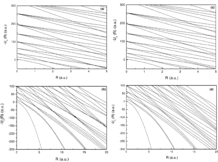
Con-sidering that different angular momentum solutions are not coupled by the interaction terms, the potential curves may cross each other. Besides, it is possible to associate the asymptotic quantum numbers with those numbers at R50, as in Eq.~31!. The eigenstates of these potential curves ob-tained from unidimensional equations are easily calculated with great precision for all of the range of the hyperradius.

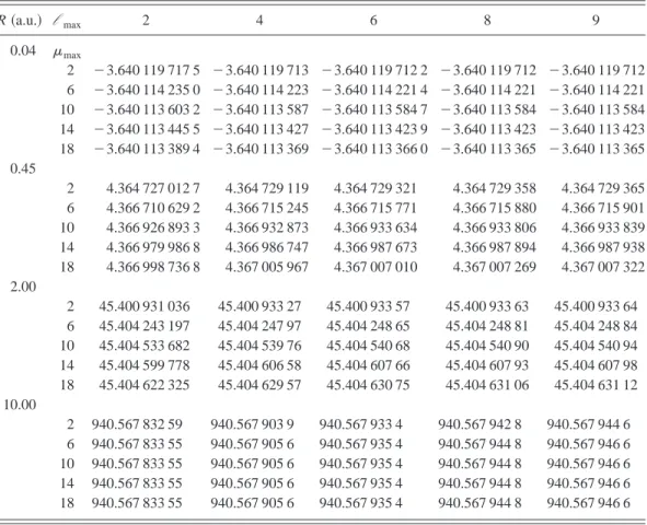
After the normalization of the angular basis functions, we proceed to the diagonalization of the total angular operator. The resulting corrected potential curves are shown in Figs. 1~c!and 1~d!and the efficiency of the process can be verified in Table I, where we show the convergence of the lowest and most important potential curve for some representative val-ues of R with the varying size of the diagonalization matrix. The maximum value of the angular momentum

l

_max is re-lated with the truncation of the expansion of the channel functions in the total angular momentum basis as given in Eq. ~13!. We can see that the convergence inmmax is very fast, for all values of

l

_{maxlisted and for all regions of R. The} angular momentum expansion is not as fast or efficient, es-pecially for the minimum of the potential curve, but the choice of the coupled angular momentum is standard in the literature as it allows the simultaneous diagonalization of the angular operators of each electron.

We note that the curves in Figs. 1~a!and 1~b! resemble those of Figs. 1~c! and 1~d!, except that the crossings are avoided in the latter. This means that Eq. ~31!is no longer valid. In the region of the avoided crossings, the angular functions have sharp transitions as the behavior of the two angular channels changes into one another. This is reflected on the nonadiabatic couplings, especially on the Q_ll8’s, which involve second derivatives of the angular functions. An example is shown in Fig. 2 where some representative couplings between the first three potential curves present peaks related to the avoided crossings of the potential curves. The avoided crossings also affect the behavior of the angular channel functions generating sharp transitions, which are not present in the physical system. Their effect is further cor-rected by the radial coefficients Fm(R) of the adiabatic

ex-pansion for each energy of the system.

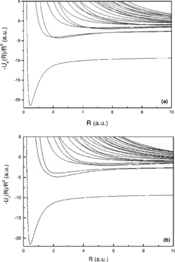
The potential curves of the Laguerre-Jacobi solutions can be compared with the exact ones in a more familiar picture when divided by R2_{, as shown in Fig. 3. We observe that,} except in the avoided-crossing regions, the deviations are more pronounced on the minimum of the potential well as expected, since the interaction potential for small and asymptotic values of R is not strongly dependent on the off-diagonal angular momentum coupling.

In order to analyze the effect of the size of the diagonal-ization basis in the angular channel functions as a function of

a, we have squared the channel function and integrated it over the spherical angles Vi5$ui,fi%, i51,2. Such a

pro-cedure is defined as follows:

Tl

max,mmax

l _~R;a!

5

E

uFl~R;a,V1,V2!u2dV1dV2. ~32!

Using the channel function corresponding to the lowest po-tential curve (l51), we have computed the functional~32!, for different values of R, using only one Laguerre-Jacobi function, labeled by the pair (

l

_max,mmax)5(0,0), and then using

l

_{max59 andmmax59. The comparison between these} two calculations is shown in Fig. 4. In this figure we can see that there is no apparent difference between both calculations for each chosen value of R. This difference is shown in detail in Fig. 5, where it can be observed that even for the mini-mum of the potential curve, about R50.45 a.u., the differ-ence between the solutions is very small. This is a strong indication of the appropriated choice of the diagonalization basis. It is important to note that the good result is due to the continuous transformation of the angular basis as the hyper-radius changes, avoiding the necessity of different ap-proaches for each region of R. An example of such a case would be the analytical solutions at R50, which fail to re-produce the asymptotic behavior, and also the hydrogenic solutions for large values of R, which lack completeness un-less the hard-dealing continuum solutions are taken into ac-count.

TABLE I. Convergence of the diagonalizing process for the first potential curve. The indicesmmaxand

l_maxare the maximum value of the Jacobi and angular momentum labels used to construct the diagonaliza-tion basis. The resulting matrix has the dimensionl _maxmmax/2 (m is even for L50, S50 states!. The point R50.45 a.u. corresponds approximately to the minimum of the potential curve well.

R~a.u.! l _max 2 4 6 8 9

0.04 mmax

2 23.640 119 717 5 23.640 119 713 23.640 119 712 2 23.640 119 712 23.640 119 712 6 23.640 114 235 0 23.640 114 223 23.640 114 221 4 23.640 114 221 23.640 114 221 10 23.640 113 603 2 23.640 113 587 23.640 113 584 7 23.640 113 584 23.640 113 584 14 23.640 113 445 5 23.640 113 427 23.640 113 423 9 23.640 113 423 23.640 113 423 18 23.640 113 389 4 23.640 113 369 23.640 113 366 0 23.640 113 365 23.640 113 365 0.45

2 4.364 727 012 7 4.364 729 119 4.364 729 321 4.364 729 358 4.364 729 365 6 4.366 710 629 2 4.366 715 245 4.366 715 771 4.366 715 880 4.366 715 901 10 4.366 926 893 3 4.366 932 873 4.366 933 634 4.366 933 806 4.366 933 839 14 4.366 979 986 8 4.366 986 747 4.366 987 673 4.366 987 894 4.366 987 938 18 4.366 998 736 8 4.367 005 967 4.367 007 010 4.367 007 269 4.367 007 322 2.00

2 45.400 931 036 45.400 933 27 45.400 933 57 45.400 933 63 45.400 933 64 6 45.404 243 197 45.404 247 97 45.404 248 65 45.404 248 81 45.404 248 84 10 45.404 533 682 45.404 539 76 45.404 540 68 45.404 540 90 45.404 540 94 14 45.404 599 778 45.404 606 58 45.404 607 66 45.404 607 93 45.404 607 98 18 45.404 622 325 45.404 629 57 45.404 630 75 45.404 631 06 45.404 631 12 10.00

2 940.567 832 59 940.567 903 9 940.567 933 4 940.567 942 8 940.567 944 6 6 940.567 833 55 940.567 905 6 940.567 935 4 940.567 944 8 940.567 946 6 10 940.567 833 55 940.567 905 6 940.567 935 4 940.567 944 8 940.567 946 6 14 940.567 833 55 940.567 905 6 940.567 935 4 940.567 944 8 940.567 946 6 18 940.567 833 55 940.567 905 6 940.567 935 4 940.567 944 8 940.567 946 6

With the angular solutions calculated, we can now solve the radial equation for the bound states of the Li1. The de-termination of the energy lines is done in a systematic way by truncating the adiabatic expansion into a maximum num-ber Nc of coupled channels. The calculated energy for each

approximation is related to the exact value in an upper and lower bound scheme @21,22#, i.e.,

«EAA<«exact<«CAA<«UAA, ~33!

where the EAA~extreme adiabatic approximation!approach corresponds to neglecting all couplings, the UAA~uncoupled adiabatic approximation!corresponds to the inclusion of the diagonal coupling, and the nondiagonal couplings are taken into account on the CAA~coupled adiabatic approximation!, approaching the exact energy as more radial channels are coupled. This behavior is clear in Table II, where the calcu-lated energy converges to the variational result @23# as the number of Nc coupled channels increases. The convergence

is not uniform because channels related with the same angu-lar momentum of the first channel are expected to give the most important contributions. With 13 coupled channels, the error obtained is less than 1 ppm. In the same table, we show that the convergence pattern is similar to the helium case @18#, even with the significative difference in the calculated energy. This suggests the use of this basis for the calculation of energies in the isoelectronic series of the helium.

FIG. 3. Comparison between potential curve wells of the Li1_.

~a!Decoupled solutions.~b!The exact solutions. The lowest poten-tial curve, which gives the bound states, is deeper for the decoupled solution than for the exact one since it does not take into account all the effects of the electron-electron repulsion. For large and small R, the differences between the solutions become smaller.

FIG. 4. Behavior of the coupled angular channel functions ~in atomic units! as given by Eq. ~32!, with (mmax,l max)5(9,9) for

different values of the hyperradius. The dots are the same calcula-tion using only the lowest basis eigenstates, which corresponds to (mmax,lmax)5(0,0).

FIG. 5. Difference between the solutions shown in Fig. 4. ~a!

The first excited-state energies are listed in Table III. They are obtained from the same set of potential curves as the ground-state energy, but there is a loss of accuracy for the lowest states due to the behavior of nonadiabatic cou-plings with R. This effect becomes less important for higher excited states, whose wave functions’ main bodies are dis-tributed over larger values of R, where the couplings are very small, as seen in Fig. 2.

V. CONCLUSION

The solution of a system of partial equations in 3N24 angular variables is a formidable and sometimes unpractical task. Direct solutions are difficult even in the N53 helium-like case. The long-range interactions cause three different regimes, in which the solutions differ totally. Aside from the spherical harmonics, the R50 free particle functions are Ja-cobi polynomials in essence. In the asymptotic region, the bound behavior will dominate ~hydrogenic in the helium case!and the intermediate region is a transition between both behaviors. Therefore, a proper numerical technique for one region will be inaccurate and instable in the other regions. These problems are significative due to the fact that channel functions and potential curves are the basic input for the

radial equations. Inaccuracies on those quantities will dete-riorate the calculation of energies and radial amplitudes.

The method of analytical expansions developed in Ref. @7#solves the problems for most of the three-body systems. The understanding that the expansion in harmonics associ-ated to the O(3N23) symmetry is not efficient even in the intermediate R-region suggested the solution of the equations by power series in an appropriated angular variable. The ex-tension of the method for more complex problems is, how-ever, unpractical. The N.3 problem requires several angular variables and therefore multivariable power expansion tech-niques are extremely difficult. However, the calculation of potential curves for N.3 can proceed by the construction of a new class of one-dimensional R-dependent functions to replace the ordinary Jacobi basis.

The eigenstates of the decoupled angular equation, the one-channel functions, fill those requirements when the vari-able z is introduced. With this varivari-able, the angular differen-tial equation for each channel may be changed to furnish polynomial solutions at the limits R50 and R→`. The use of the Frobenius method leads to very fast convergent expan-sions of the eigenstates in the full R region. The main aspect of the angular basis constructed with these functions is the update of the basis with R as it carries the information of the diagonal components of the interaction. The result of this procedure is the fast convergence in all of the diagonaliza-tion process, especially at the dissociadiagonaliza-tion region. For the positive ion of the lithium, the energy obtained with these potential curves has an accuracy of a few parts per million.

In this paper, we show a significant gain in efficiency diagonalizing the angular heliumlike atom equation with the one-channel basis instead of the pure hyperspherical harmon-ics. The hope to use it for the many-body problem functions generated by the three-body problems lies in the fact that the kinetic-energy operator in hyperspherical coordinates is con-structed recursively from lower dimensions to higher ones.

ACKNOWLEDGMENTS

This work was supported by the Brazilian Agencies Con-selho Nacional de Desenvolvimento Cientı´fico e Tecno-lo´gico ~CNPq!and Fundac¸a˜o de Amparo a` Pesquisa do Es-tado de Sa˜o Paulo ~FAPESP!, Processes Nos. 98/03044-7 and 97/06271-1.

TABLE II. Ground-state energy@«0~a.u.!#convergence of the

Li1_{as a function of the number N}

cof coupled angular states in the

radial equations. It used 30 coupled angular momenta for the first potential curve and for the corresponding diagonal nonadiabatic coupling Q11. All other potential curves were obtained using 10

coupled angular momenta. The first row, 1*, corresponds to the lower bound calculation ~EAA approach!. The variational result («var) is from Ref.@23#. The convergence follows a similar pattern

to that observed for the He atom@18#.

Nc Energy (2«0) («var2«0)/«var~ppm! He@18#

1* 7.332 345 38 27 202.28 29 060.02

1 7.262 640 06 2 372.74 2 813.91

2 7.267 016 80 1 771.53 1 748.85

3 7.279 704 90 28.64 38.88

4 7.279 731 28 25.02 31.66

5 7.279 734 27 24.60 30.30

6 7.279 756 47 21.55 22.69

7 7.279 897 74 2.15 2.52

8 7.279 897 78 2.14 2.50

9 7.279 897 90 2.13 2.46

10 7.279 897 92 2.13 2.45

11 7.279 897 97 2.12 2.42

12 7.279 898 42 2.06 2.22

13 7.279 909 25 0.57 0.48

14 7.279 909 26 0.57

15 7.279 909 27 0.57

16 7.279 909 28 0.56

17 7.279 909 28 0.56

18 7.279 909 29 0.56

19 7.279 909 29 0.56

20 7.279 909 31 0.56

21 7.279 910 83 0.35

TABLE III. Lowest binding energies, « ~a.u.!, of the Li1 _for Nc521 coupled angular states in the radial equations compared

with the variational energies «var from Ref. @24#, except for the ground-state energy, which is from Ref.@23#.

State

Energy (2«)

Variational (2«var) @24#

(«var2«)/«var ~ppm!

1s1s 7.279 910 8 7.279 913 39 0.35

1s2s 5.040 865 9 5.040 876 74 2.15

1s3s 4.733 725 0 4.733 756 6.55

1s4s 4.629 749 1 4.629 783 7.34

@1#C.D. Lin and X. Liu, Phys. Rev. A 37, 2749~1988!.

@2#J.J. De Groote, J.E. Hornos, H.T. Coelho, and C.D. Caldwell, Phys. Rev. B 46, 2101~1992!.

@3#O.I. Tolstikhin, S. Watanabe, and M. Matsuzawa, Phys. Rev. Lett. 74, 3573~1995!.

@4#J. Brust and C.H. Greene, Phys. Rev. A 56, 2005~1997!.

@5#S. Schmatz and D.C. Clary, J. Chem. Phys. 110, 9483~1999!.

@6#J.H. Macek, J. Phys. B 1, 831~1968!.

@7#J.E. Hornos, S.W. MacDowell, and C.D. Caldwell, Phys. Rev. A 33, 2212~1986!.

@8#A.G. Abrashkevich, D.G. Abrashkevich, M.I. Gaysak, V.I. Lendyel, I.V. Puzynin, and S.I. Vinitsky, Phys. Lett. A 152, 467~1991!.

@9#J.Z. Tang, S. Watanabe, and M. Matsuzawa, Phys. Rev. A 46, 2437~1992!.

@10#C.D. Lin, Phys. Rep. 257, 1–83~1995!.

@11#C.D. Lin, Phys. Rev. A 57, 4268~1998!.

@12#Yu.F. Smirnov and K.V. Shitikova, Fiz. Elem. Chastits At. Yadra 8 847~1977! @Sov. J. Part. Nucl. 8, 344~1977!#.

@13#E. Santopinto, F. Iachello, and M.M. Giannini, Eur. Phys. J. A

1, 307~1998!.

@14#L.V. Grigorenko, B.V. Danilin, V.D. Efros, N.B. Shul’gina, and M.V. Zhukov, Phys. Rev. C 60, 44 312~1999!.

@15#H.T. Coelho, J.J. De Groote, and J.E. Hornos, Phys. Rev. A 46, 5443~1992!.

@16#J.J. De Groote, A.S. dos Santos, M. Masili, and J.E. Hornos, Phys. Rev. B 58, 10 383~1998!.

@17#M. Masili, J.J. De Groote, and J.E. Hornos, Phys. Rev. A 52, 3362~1995!.

@18#J.J. De Groote, M. Masili, and J.E. Hornos, J. Phys. B 31, 4755

~1998!.

@19#Handbook of Mathematical Functions, 3rd ed. edited by M.

Abramowitz and I. A. Stegun~Dover, New York, 1965!.

@20#J. Macek, Phys. Rev. A 31, 2162~1985!.

@21#H.T. Coelho and J.E. Hornos, Phys. Rev. A 43, 6379~1991!.

@22#A.F. Starace and G.L. Webster, Phys. Rev. A 19, 1629~1979!.

@23#G.W. Drake, Can. J. Phys. 66, 586~1988!.

@24#Y. Accad, C.L. Pekeris, and B. Schiff, Phys. Rev. A 4, 516