Minimal Feature set for Unsupervised Classification of Knee
MR Images
Ms. Rajneet Kaur1 and Dr. Naveen Aggarwal2
1
Assistant Professor, Sri Guru Granth Sahib World University, Fatehgarh Sahib
2
Assistant Professor, University Institute of Engineering & Technology, Panjab University
Abstract
Knee scans is very useful and effective technique to detect the knee joint defects. Unsupervised Classification is useful in the absence of domain expert. Real Knee Magnetic Resonance Images have been collected from the MRI centres. Segmentation is implemented using Active Contour without Edges. DICOM, Haralick and some Statistical features have been extracted out. A database file of 704 images with 46 features per images has been prepared. Unsupervised Classification is implemented with clustering using EM model and then classification using different classifiers. Learning rate of 5 classifiers (ID3, J48, FID3new, Naive Bayes, and Kstar) has been calculated. At the obtained learning rate minimal feature set has been obtained for unsupervised classification of Knee MR Images.
Keywords: Unsupervised Classification, Segmentation, Feature Extraction, Knee MR Images.
1. INTRODUCTION
MRI is one of the latest medical imaging technologies. An MRI (Magnetic Resonance Images) scan is a radiology technique that uses magnetism, radio, electric waves and a computer technology to produce images of body structure. The Magnetic resonance imaging used for Knee scans is very useful and effective technique to detect the knee joint defects. It is a non-invasive method to take picture of knee joint and the surrounding images. Images are produced and analysis is done on one image at a time. Radiologist diagnose whether the image is normal or abnormal. He does not give collective analysis of many images at a time. In other words current medical technologies are not used for analysis purpose of multiple images and to give informative result about those images together at a time which can be helpful in future. This is what data mining used for. Along with this because of busy schedules
of radiologists, it is difficult to go through large number of images every day. So an Unsupervised Classification of MRI image is used for discovering meaningful patterns and relationships that lie hidden within very large database in the absence of radiologist.
2. SEGMENTATION
Segmentation is the first step in the process of classification of images. Segmentation algorithms varies from edge based, region based and other thresholding techniques. In computer vision, segmentation refers to the process of partitioning a digital image into multiple segments (sets of pixels, also known as super pixels). The goal of segmentation is to simplify and/or change the representation of an image into something that is more meaningful and easier to analyze [1]. Image segmentation is typically used to locate objects and boundaries (lines, curves, etc.) in images. More precisely, image segmentation is the process of assigning a label to every pixel in an image such that pixels with the same label share certain visual characteristics.The result of image segmentation is a set of segments that collectively cover the entire image, or a set of contours extracted from the image (see edge detection). Each of the pixels in a region is similar with respect to some characteristic or computed property, such as color, intensity, or texture. Adjacent regions are significantly different with respect to the same characteristic.
2.1 IMPLEMENTATION OF
SEGMENTATION
Distance map of initial mask: Chan and Vese have used phi0 which is a distance map of initial mask in his work, but we can modify it to phi1, because converting image to double and then adding to phi calculation does not make any difference. So we can emit this parameter and shorten the equation.
phi0 = bwdist(m)-bwdist(1-m)+im2double(m)-.5; phi1 = bwdist(m)-bwdist(1-m)-.5;
subplot(2,2,1); plot(phi0),title('phi0'),subplot(2,2,2); plot(phi1),title('phi1');
Figure 1: Distance Mask Of initial Mask
MRI images are larger in size. In order to process
them it is needed to change the value of parameter μ
if μ is small, then only smaller objects will be detected if μ is larger, then it will work for larger objects also or objects formed by grouping.
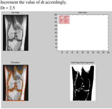
Figure 2: ‘chan’ or ‘vector’ method at dt=0.5
Increment the value of dt accordingly. Dt = 2.5
Figure 3: ‘chan’ or ‘vector’ method at dt=2.5
The output obtained by both ‘chan’ and ‘vector’ method is approximately same. But the difference in both the methods is this that if image is noisy then ‘vector’ method gives better result than the ‘chan’ method. So in the case of noisy images it is preferable to use ‘vector’ method.
2. ‘Multiphase’ method: In the case of ‘multiphase method:
Four regions aa1, aa2, aa3 and aa4 together form the complete segmented image. We can extract each region separately. By separating each region part we can get our region of interest without applying any other technique on segmented image.
(a) (b)
(c) (d)
Figure 5: Sub regions of Active Contour without edge
3. FEATURE EXTRACTION
Large number of algorithms has been proposed for the extraction of features from knee MRI images. Texture analysis serve as a base for various feature description. Statistical, structural, spectral, filtering, histograms, transformation and many more methods are used for texture feature extraction. The global features capture the gross essence of the shapes while the local features describe the interior details of the trademarks. In the feature extraction part total 45 features have been extracted from Knee MRI images. Out of which 19 are DICOM images header features [4], 13 are haralick texture features [5] and rest are images statistical features [6]. DICOM header features are extracted out in order to check either all images have been taken under similar environmental conditions or not.
Features extracted:
Following 46 features per file comprises database file-
1.File Size 17.Flip Angle 2.Width 18.Rows 3.Height 19.Colums
4.Bit Depth 20.Angular Moment 5.PatientName 21.Contrast
6.Patient Birth Date 22.Correlation 7.Patient Sex 23.Entropy
8.Patient’s Age 24.Inverse Difference Moment 9.Patient’s Weight 25.Sum Average
10.Body part examined 26.Sum Variance 11.Slice Thickness 27.Sum Entropy 12.Image Frequency 28.Difference Average 13.Image Nucleus 29.Differnce Variance 14.Magnetic Field Strength 30.Differnce Entropy
15.Spacing between Slices 31.Infoiormation of Correlation1 16. Pixel Bandwidth 32.Infoiormation of Correlation2
4. UNSUPERVISED CLASSIFICATION
Classification is a process which is used to categorize the data (XML, images, text etc) into different groups (“classes”) according the similarities between them [7]. Image classification is defined as the process to classify the pixels of images into different classes according to similarity.
latent variables, and maximization (M) step, which computes parameters maximizing the expected log-likelihood found on the E step. These parameter-estimates are then used to determine the distribution of the latent variables in the next E step.
Clustering has been implemented. The data is divided into different clusters and we saved the cluster assignment file in ‘ARFF’ format, whose last attributes shows the cluster assignment. The generated clustered file is used as input for classification in the next phase. Algorithms ‘ID3’, ‘J48’, ‘FID3new’, ‘Naive Bayes’ & ‘Kstar’ has been implemented and results are recorded and studied for analysis purpose. FID3new is an algorithm which is made by combining the two algorithms ID3 and FT, so it is a hybrid algorithm. In this the information gain and entropy measure of attributes is calculated according to ID3 algorithm and then put as input for the classification and the further classification is done according to FT algorithm. Improved results have been obtained on our dataset.
4.1 IMPLEMENTATION
Knee MRI scans has been collected and after image processing total 46 features have been extracted from the Knee MR images .A database file of 704 tuples and 46 attributes has been made in ASCII in CSV format, then conversion of this file to CSV file is done. CSV files are readable in Weka [9]. The generated CSV file is opened in Weka and then different processes like data cleaning, data processing and data transformation are applied on to the input database file. These steps act as pre-processing steps for the classification of data. Along with this attribute removal is also done. Some of the attributes like patient’s name, patient weight, body part examined etc are removed as they contribute nothing in classification process. Classification is implemented using ‘ID3’, ‘J48’, ‘FID3new’, ‘Naive Bayes’ & ‘Kstar’ and results are recorded and studied for finding the minimal feature set for unsupervised classification.
In order to find out minimal features set for Knee MR Images in case of supervised classification, first step is to find out the learning rate of different algorithms. To find out the learning rate of different algorithms, the training is started from 1 % percentage split and keeps on increasing till 99% percentage split. Results of different algorithms have been recorded and analysed and interpretation has been done according to the analyses.
4.1.1 COMPARISON OF TP RATE VS
PERCENTAGE SPLIT OF DIFFERENT
ALGORITHMS FOR UNSUPERVISED
CLASSIFICATION
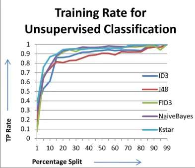
Clustering is implemented on original database file with EM clustering algorithm. Output file is saved in ARFF format and given as input during classification. Training rate is started from 1% and gradually increased by 5 in each iteration till 99% of training. TP Rate of different algorithms has been calculated and plotted below. All algorithms behave differently according to their working.
It is observed that at 50% percentage split ID3 & FID3new gives TP Rate of 1 and gives constant value. All other algorithms also gives value near to 1 and get stabilized at this value. So we can say that 50% of training is required in case of unsupervised Classification. This is the minimum and required training which is must in order to get the proper and correct results. If we keep on increasing the value of training rate from 50 %, then there are almost same values obtained over all other percentage splits.
In case of FID3new after 50 % near about 90 % the TP rate goes below the value specified at 50% of percentage split. This is because of the over training. So we can say that 50 % is the required training in case of supervised classification.
Figure 4.1: Training rate for unsupervised classification 0
0.1 0.2 0.3 0.4 0.5 0.6 0.7 0.8 0.9 1
1 10 20 30 40 50 60 70 80 90 99
T
P
Ra
te
Percentage Split
Training Rate for
Unsupervised Classification
ID3
J48
FID3
NaiveBayes
4.1.2 COMPARISON OF FP RATE VS
PERCENTAGE SPLIT FOR
UNSUPERVISED CLASSIFICATION
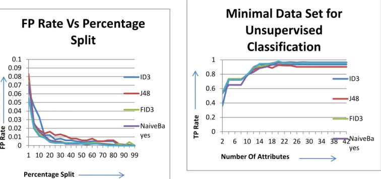
FP Rate of different algorithms has been calculated and plotted below. In this graphs training rate is started from 1% and then we keep on increasing the training rate by 5 in each step and continue till 99 % of training. All algorithms behaves differently according to their working
It has been concluded from the above graph that at 50% percentage split ID3 & FID3new gives FP Rate of 0 and gives constant value. All other algorithms also gives value near to 0 and get stabilized at this value. So we can say that 50% of training is required in case of Supervised Classification. This is the minimum and required training which is must in order to get the proper and correct results. If we keep on increasing the value of training rate from 50 %, then there are almost same values obtained over all other percentage splits.
In case of FID3new after 50 % the FP rate sometime goes above the value specified at 50% of percentage split. This is because of the over training. So we can say that 50 % is the required training in case of supervised classification.
Figure 4.2: FP Rate Vs Percentage Split
In brief 50% of training is required in case KNEE Magnetic Resonance Images. At this percentage split of training minimal feature set for KNEE images has been obtained for unsupervised classification.
4.1.3 MINIMAL FEATURE SET FOR
UNSUPERVISED CLASSIFICATION
Training of 50% is required in case of unsupervised classification. To find out minimal feature set, start the evolution from 2 attributes and increase the number by 2 in every step till all 41 attributes has not covered.
It has been observed from the plotted values that at 20 attributes all algorithms give maximum value of TP Rate. After 10 attributes ID3, FID3new and J48 gives constant value as they get stabilized, however the value of Naive Bayes and Kstar decreases. This is because of the over fitting of data. Over fitting occurs when the information available for proper classification is more than the required one. Other reason for over fitting is that during the training phase data is trained on different data, whereas its evaluation is done on some unknown data.
Most of the classifiers start memorizing the training data rather than to generalize them which results in over fitting of the data.
Figure 4.3: Minimal feature set for unsupervised classification
0 0.01 0.02 0.03 0.04 0.05 0.06 0.07 0.08 0.09 0.1
1 10 20 30 40 50 60 70 80 90 99
F
P
Ra
te
Percentage Split
FP Rate Vs Percentage
Split
ID3
J48
FID3
NaiveBa
yes 0
0.2 0.4 0.6 0.8 1
2 6 10 14 18 22 26 30 34 38 42
T
P
Ra
te
Number Of Attributes
Minimal Data Set for
Unsupervised
Classification
ID3
J48
FID3
5. CONCLUSION
Real Knee MRI data have been collected from MRI canters. Segmentation is implemented using Active Contour without edges. It is easy to separate them out easily and can easily access the part containing cartilage thickness. In the next phase, total 46 features have been calculated and in the pre-processing 5 features which give the detail of patient’s personal data have been removed. A database file consisting of 704 images with 41 lists of attributes is prepared and it used for classification process in next phase. Classification is implemented and performance of different parameters are compared using five algorithms ‘ID3’, ‘J48’, ‘FID3new’, ‘Naive Bayes’ & ‘Kstar’. ‘FID3new’ is a hybrid algorithm, which is proposed in this work. . In unsupervised classification learning rate of different algorithms is calculated by starting the training from 1 % till 99 % and it has been concluded that minimum 50% of training is required in the case of unsupervised classification also. At this training rate minimal feature set has been calculated by taking minimum 2 features in starting and then increase the number two in each iteration till 42 features (one more feature that defines the cluster assignment). In case of unsupervised classification minimal feature set consist of 20 features and ‘slice thickness’ is the feature with highest priority. Classification is done using different algorithms. It has been concluded that ‘FID3new’ correctly classifies all instances and gives TP rate of 1 and Root Means Square’s Error value 0. It classify the database on the base of feature ‘Slice thickness’ and divides them into four classes A, B, C & D. Where A= 0.9 mm, B=3, C= 4 and D= 6. The images coming under B & D class is classified as ‘Normal’ images and the images coming under A & D class is classified as ‘Abnormal’ images
6. FUTURE WORK
Only on 704 knee MR Images. Database can be extended and same methodology can be applied to the database containing images in thousands and many more. Only MRI Knee data has been used, the same approach can be extended to different medical imaging technologies like CT scan etc. Different segmentation algorithms can be used for segmentation. More features like Zernike moments etc can be calculated and feature set can be extended. Similarly for classification different combination of algorithms can be tried and results can be compared, if any improvements will be there, then it can be suggested.
7. REFERENCES
[1]Qi Luo,Wuhan,“Advancing Knowledge Discovery and Data Mining", Procedings of Knowledge Discovery and Data Mining,IEEE WKDD, pages 3-5, ISBN: 978-0-7695-3090-1, 2008
[2] T. Chan and L. Vese, “Active contours without edges,” in IEEE Trans on Image Processing Vol 10,pages 266-278, ISBN: 1057-7149, 2001.
[3]D. Mumford and J. Shah, “Optimal approximation by piecewise smooth functions and associated variational problems”, Commun. Pure Appl. Math, vol. 42, pages 577–685, 1989.
[4] Rosset, A. Spadola, L. Rati., “OsiriX: An Open-Source Software for Navigating in Multidimensional DICOM Images”, JOURNAL OF DIGITAL IMAGING, vol 17, part 3, pages 205-216, ISBN: 0897-1889 , W B SAUNDERS CO, 2004.
[5] R. M. Haralick and K. Shanmugam, "Computer Classification of Reservoir Sandstones," IEEE Transactions on Geoscience Electronics, vol. 11, pages. 171-177, 1973.