Location analysis of city sections

Location analysis of city sections

Socio-demographic segmentation and restaurant

potentiality estimation

–

A case study City of Lisbon

Location analysis of city sections

Socio-demographic segmentation and restaurant potentiality

estimation

–

A case study City of Lisbon

Dissertation supervised by:

Professor Roberto Henriques, PhD

Professor Marco Painho, PhD

Professor Jorge Mateu, PhD

AKNOWLEDGEMENTS

I would like to express full appreciation and gratitude to Consortium of Master’s program Geospatial Technologies for enabling me to be funded throughout my studies and thus giving me the opportunity to achieve this master’s degree.

Secondly, I would like to thank to my family, for support, trust and belief in my success. In addition, I am grateful to my supervisor and co-supervisors for sharing with me an immodestly meaningful feedbacks for the improvement of the thesis.

Special thanks to PhD candidate Fernando Santa for statistical support, Yash Bonno for advises.

Location analysis of city sections

Socio-demographic segmentation and restaurant potentiality

estimation

–

A case study City of Lisbon

ABSTRACT

One of the objectives of this study is to perform classification of socio-demographic

components for the level of city section in City of Lisbon. In order to accomplish suitable platform for the restaurant potentiality map, the socio-demographic components were selected

to produce a map of spatial clusters in accordance to restaurant suitability. Consequently, the second objective is to obtain potentiality map in terms of underestimation and overestimation

in number of restaurants. To the best of our knowledge there has not been found identical methodology for the estimation of restaurant potentiality. The results were achieved with

combination of SOM (Self-Organized Map) which provides a segmentation map and GAM (Generalized Additive Model) with spatial component for restaurant potentiality. Final results

indicate that the highest influence in restaurant potentiality is given to tourist sites, spatial autocorrelation in terms of neighboring restaurants (spatial component), and tax value, where

KEYWORDS

Location Analysis

Exploratory Analysis

Self-Organized Maps

Spatial Weighting

Generalized Linear Model

General Additive Model

Predictive Modelling

R

ACRONYMS

SOM

–

Self Organized Maps

GLM

–

Generalized Linear Model

GAM

–

Generalized Additive Model

EDA

–

Exploratory Data Analysis

ESDA

–

Exploratory Spatial Data Analysis

U-matrix

–

Unified Distance Matrix

BMU

–

Best Matching Unit

AIC - Akaike Information Criterion

BIC

–

Bayesian Information Criterion

ANOVA

–

Analysis of Variances

CV

–

Cross validation

REML - Residual Maximum Likelihood

IRLS - Iteratively Reweighted Least Squares

RMSE

–

Root Mean Square Error

INDEX OF TEXT

AKNOWLEDGEMENTS ... iii

ABSTRACT ... iv

KEYWORDS ... v

ACRONYMS ... vi

INDEX OF FIGURES ... viii

INDEX OF TABLES ... x

1 INTRODUCTION ... 1

1.1 Overview ... 1

1.2 Objectives ... 3

2 THEORETICAL FRAMEWORK ... 4

2.1 Related work ... 4

2.2 Exploratory spatial data analysis and Self Organized Maps ... 4

2.2.1 Exploratory spatial data analysis and descriptive statistic tools ... 4

2.2.2 Self-Organized Maps ... 5

2.2.3 Spatial clustering – autocorrelation test ... 8

2.2.4 SOM - related applications ... 8

2.3 Prediction Examination ... 9

2.3.1 Generalized Linear Model ... 10

2.3.2 Poisson distribution ... 10

2.3.3 Generalized Additive Model ... 11

2.3.4 Methods for spatial aggregation of neighbourhoods ... 11

2.3.5 Spatial weights ... 13

2.3.6 Spatial autocorrelation test... 13

2.3.7 Model selection ... 15

2.3.8 Predictive approaches - related applications ... 16

3 STUDY AREA ... 18

4 METHODOLOGY ... 19

4.1 Dataset ... 20

4.1.1 Data pre-processing ... 21

4.1.2 Data normalization... 22

4.1.3 Analysis Approach... 22

4.1.4 Base model construction ... 26

5 RESULTS AND ANALYSIS ... 28

5.1 Socio-demographic segmentation ... 34

5.1.1 Input parameters ... 34

5.1.2 Process ... 35

5.1.3 Clusters’ analysis ... 39

5.2 Predictive modelling ... 40

5.2.1 Machine learning ... 40

5.2.2 Regression models ... 42

5.2.3 Neighbourhood criteria ... 46

5.2.4 Spatial model construction... 48

5.2.5 Model selection ... 49

5.3 Restaurant potentiality estimation ... 51

6 FINAL ANALYSIS AND DISCUSSION ... 52

7 CONCLUSION AND FUTURE WORK ... 57

BIBLIOGRAPHY... 59

ANNEX 1 ... 62

ANNEX 2 ... 62

ANNEX 3 ... 63

ANNEX 4 ... 64

ANNEX 5 ... 70

ANNEX 6 ... 72

INDEX OF FIGURES

Figure 1: Population, Budget, Jobs in Portugal. Data derived from INE ... 1

Figure 2: SOM illustration: Example of three dimensionality towards two dimensionality [25]... 6

Figure 3: Typical types of topology for neighbours and borders) [25] ... 6

Figure 4: SOM steps - best matching unit and input dataset ... 6

Figure 5: Training progress and mean distance to closest unit ... 7

Figure 6: Queen's (left) and Rook's contiguity (right) ... 12

Figure 7: Delaunay (left), Voronoi (right) – Source: wolfram.mathworld ... 12

Figure 8: MEM for regular (up) and irregular (bottom) network ... 15

Figure 9: Study area – Lisbon ... 18

Figure 10: General Flowchart ... 19

Figure 11: Descriptive statistics ... 22

Figure 12: Flowchart - SOM ... 23

Figure 13: Flowchart - Predictive modelling ... 25

Figure 14: Flowchart - Cut-offs ... 27

Figure 15: Density of tourist sites ... 28

Figure 16: Density of restaurants ... 29

Figure 17: Parallel coordinates - all variables ... 30

Figure 18: Boxplots ... 31

Figure 19: Boxplots ... 32

Figure 20: Histograms ... 32

Figure 21: Scatterplots ... 33

Figure 22: Coefficient - Pearson's correlation (left), Spearman’s correlation (right) ... 33

Figure 23: Codebook vectors for 256 neurons with 14 variables ... 35

Figure 24: Number of city sections per neuron (left), Node Quality (right) ... 35

Figure 25: Number of iterations (Left), Number of clusters (Right) ... 36

Figure 26: Dendogram ... 36

Figure 27: Component planes ... 37

Figure 28: U-matrix ... 37

Figure 29: Clusters ... 38

Figure 30: Compared smoothness of covariates ... 43

Figure 31: REML diminish effect on covariates ... 45

Figure 32: Effect of covariates ... 45

Figure 33: 2 nearest neighbour polygons relationship ... 46

Figure 34: Moran global test for spatial autocorrelation – KNN2... 47

Figure 35: Local neighbourhoods of Moran I test ... 47

Figure 36: Effect of spatial covariate ... 49

Figure 38. Histogram of deviations ... 51

Figure 39: Deviance residuals distribution with cut-offs values ... 52

Figure 40: SOM clusters and thematic map ... 53

Figure 41: Cluster map with restaurants density ... 54

Figure 42: Cluster map with tourist site densities ... 55

INDEX OF TABLES

Table 1: Selected variables from Census 2011 ... 20

Table 2: Tourists sites – totals ... 21

Table 3: Selected variables for each SOM model ... 24

Table 4: Parallel plots: an optimized city section in Lisbon ... 31

Table 5: SOMs specification ... 34

Table 6: Cluster analysis ... 38

Table 7: Machine learning results: accuracy and RMSE ... 42

Table 8: Base GLM model estimated coefficients ... 43

Table 9: Base GAM significance of smooth terms ... 44

Table 10: AICc values from neighbourhood matrices ... 46

Table 11: Spatial GAM ... 49

Table 12: Summary of candidates ... 49

Table 13: ANOVA test ... 50

Table 14: ANOVA test for spatial models ... 50

Table 15: Results from validation of 20% ... 50

Table 16: Summary for deviance residuals of restaurants ... 51

1

INTRODUCTION

1.1

Overview

One of the most visited and most attractive European cities in 2015 was Lisbon [1]. In 2009 it

was the 7th _{most visited city in Southern Europe [2]. The reason for attraction can be firstly due}

to its affordability when compared to other European capitals with its; beautiful antique majestic houses and buildings in downtown districts, rich history, warm climate particularly

during the winter, closeness to the beaches, food and many other things [3]. Tourism as well as the service industry in general significantly contributes to the economy both at the local and

state level. This is shown in the fact that it was recorded that tourism contributes approximately 330,000 direct jobs and 900,000 jobs indirectly thus representing about 20% of the total

employment, which is approximately 20 billion euros of annual income in Lisbon and Portugal (Figure 1) [4].

Figure 1: Population, Budget, Jobs in Portugal. Data derived from INE

In addition, population of Lisbon's metropolitan area is 2.822 million and thereabout 1/3 of the total population in Portugal; therefore the tourism industry is important in Lisbon [5].

Restaurants are one of the contributors in the hospitality and tourism industry overall [6]. The locations of restaurants with novelty and strangeness of the tourist sites are inseparable, thus

they have to be considered and analysed together [7]. Therefore the primary question is - to what extent does the influence of tourist sites impacts on the location of restaurants? Certainly

one of the most important factors is demography of the site itself with specific information about the age, employment status, sex, income [8]. Indeed, there are also many other

non-demographic important decisions that have to be considered in order to estimate a location for restaurant such as: crime rate, visibility, area traffic, ease of access, parking, area zoning,

advertisement and type of cuisine [9] [10]. Locating the most convenient site for a restaurant requires time and tedious work where stakeholders have to analyse the site and come up with a number of well justified factors with specified weights for each factor in order to determine the

79% 21%

Population

Portugal Lisbon Metropolian

85% 15%

Budget

All Tourism

81% 14%5%

Jobs

most suitable location [11]. The main reason why most of the factors have not been included in further analyses is due to the lack of data. Thus the proposed solution can be useful in the scenarios where cities or urban settlements do not have much useful public data such as:

purchasing index, lifestyle data, food and beverage purchasing index and so forth.

The analyses presented in this paper take advantage of the existence of secondary data about

city districts and try to re-evaluate the potentiality for restaurants. Ultimately the proposed method should determine the potentiality of restaurants in the city section (Portuguese: seções).

Thus in the proposed method, location analysis is conducted in the way of spatial clustering with assistance of Self-Organized Maps. The totals of tourist sites and restaurants are taken into

account for the potentiality assessment on the city section level of detail. Conducted location analysis of the city section provides socio-demographic definition of the city sections and also

estimates the potentiality of restaurants. The proposed method for the potentiality is applied by taking into account a spatial autocorrelation of the restaurants. The prediction methods such as

Generalized Linear Model (GLM) and General Additive Model (GAM) both alone and with spatial components were tested. We propose that from the best selected method the cut-offs

1.2

Objectives

The research objectives are initially based on assumptions with assistance from demographic

variables from Census data 2011. Thanks to experts and examples from [9], some assumptions can be made as following:

 Age and employment might affect restaurants visits

 City sections with college educated persons indicate an increased likelihood of higher

income.

 High tourist index leads to an increased number of restaurants

 People who work in the tertiary sector are more likely to visit restaurants

 Tax value defines the economic strength of city sections [12], hence it automatically

influences on the suitability of restaurants

 Newer residential buildings indicate the location of younger and richer families – target

group for restaurants

The assumptions helped to select suitable and appropriate variables for further analyses about the city sections. However, the census data does not contain a wealth of information about

socio-demographic components in Portugal that directly relate to the suitability of restaurants, but it provides general insight about the city section (Portuguese: seção). Consequently the

following objectives were identified:

 Undertake a segmentation of city sections with cluster analyses and identify the clusters

with restaurant potential.

 Conduct the prediction analysis to determine the potentiality of city sections for the

restaurants and examine the degree of contribution of covariates in the method used.

The following questions that may occur throughout analysis are: Which sites have higher

potentiality of restaurants, but with non-tourist influence? What socio-demographic combination of covariates may influence suitability of restaurants? Regardless, the aim is to highlight the sections which can be potential for restaurants, but without performing an in-depth

analysis about individual city section. The reason to disengage the factors from [9] provided is due to the lack of information. Hence the variables that provide National Statistical Institute of

Portugal (INE) were analysed as an implicit or an explicit implication for restaurant suitability. In reaching these objectives, this document presents a review of the implemented methods and

related work in terms of segmentation and potentiality in section 2. In the following section 3 the study area is described and an explanation of the city divisions provided. The methodology

is presented in section 4. Section 5 conveys the results, in particular the segmentation analysis and results from prediction, while in section 6 were analyzed together. Finally, in section 7 the

2

THEORETICAL FRAMEWORK

2.1

Related work

To the best of our knowledge, limited focus has been given to the estimation of site potentiality

of the restaurants on the level of city section, district, block, census track or similar subdivisions. Some of the reports are related to potentiality of the restaurant revenue by

implementing machine learning methods [13]. Others are based on restaurant ratings and popularity [14]. Some experts mention the use of applying Multi Criteria Analysis (MCA) for

site suitability [8]. The MCA methods can be time-consuming caused by associating weights to the specific module which requires questionnaires and meetings with catering, restaurateurs

and experts. Therefore even a small change can affect the final location [15] [16].

A number of papers give analysis about fast-food restaurants and neighbourhoods [17].

However, fast-food restaurants in this analysis are deliberately avoided due to the fact that they are widely distributed all over the city. In other words a vast majority of people can afford to

visit and buy a meal in fast-food restaurants. Primarily, we want to narrow down possible customers, therefore non-fast food restaurants are included in this analysis. With spatial analysis from [18] of cafe shops, a customer segmentation is considered, however the results

were biased since the site selection criteria were customized for a certain brand and it relied on MCA, also. Hence the method can depend on subjective decisions and requires decision-makers

to assign weighs for every factor.

2.2

Exploratory spatial data analysis and Self Organized Maps

Along with introduction into a problem, it is important to identify the components and obtain

an understanding of the dataset. Consequently, exploratory data analysis were conducted for an in-depth analysis of variables in order to appropriately select those for Self-Organized Map clustering. In addition, spatial autocorrelation and spatial dependency has to be explored, since

areal entities are being used.

2.2.1

Exploratory spatial data analysis and descriptive statistic tools

Exploratory data analysis (EDA) describes a set of methods for assessing features of the data and to identify patterns within a dataset. It is meaningful for problem definition since it enables

one to combine graphical and numerical statistical analyses. This allows one to discuss the

patterns and develop solutions to the problem [19]. Apart from EDA, exploratory spatial data analysis (ESDA) would need to be utilized to obtain a visual interpretation of features’ geographical distributions, taking into account spatial proximity as well as an importance of

spatial autocorrelation based on Tobler’s I Law of Geography [20]. The set of dynamic graphical methods that may be applied into the dataset variables are histograms, scatterplots,

implicitly spatially related component planes and I Moran Local test to obtain results for spatial autocorrelation among restaurants and tourist sites. A set of thematic maps may also be used to conduct descriptive statistics.

Histograms: Widely used density estimators. The horizontal axis represents bins defined as intervals and vertical axes volume of it. It estimates probability of distribution of continuous

variables [21].

Scatterplots: Prints values, typically from two variables where the horizontal axis indicates

values from one variable and the vertical axis has values from another variable. The points appear as scattered; hence it gained the name scatterplot.

Boxplot: It is used for non-parametric numeral values. It depicts data with a rectangle where

the bottom and upper line represents quartiles, while the horizontal line within the rectangle represents the median. Points outside the boxplot - whiskers are possible outliers [22].

Parallel coordinates: This is an alternative way to visualise multidimensional data. The horizontal axis represents each variable from the dataset and the vertical parallel axis indicates

the range of values for the specific variable.

Q-Q plots: In our case these will be applied for deviance residuals distribution. It plots the

quantiles of the dataset with quantiles of normal distribution. It indicates whether the scale and skewness of two datasets have similarities.

Kernel density estimators: A non-parametric estimator for probability density function (PDF) It is applied for continuous data. An important step is to choose the best bandwidth which

usually depends on the number of bins, minimum and maximum value among other things. At the beginning we applied kernel density for mapping density of restaurants and tourist sites and afterwards for setting up threshold for cut-offs from deviance residuals of predicted and existing

number of restaurants.

For the purpose of ESDA, provided tools were implemented in order to assist in establishing

segmentation analysis of clusters associated with city districts.

2.2.2

Self-Organized Maps

SOM belongs to the family of methods from an artificial neural network. It was first presented

by Finish scientist Kohonen in the early 80s [23]. The method is primarily clustering solution for multidimensionality approximation into two dimensions. The ultimate purpose of SOM is

dimensionality reduction [24] [25]. Two dimensions provide more effective visualization effect of spatial data [26] [27]. The other main characteristic in regards to SOM is that it belongs to unsupervised learning. It does not require training dataset to adjust and classify data. Output

networks contain nodes, so if it is two dimensional, the network is defined with a rectangular

For the input data the chosen winning nodes will be based on similarities. Thus, it is common to compare SOM to typical clustering method, such as k-means.

Figure 2: SOM illustration: Example of three dimensionality towards two dimensionality [25]

The importance of SOM is to preserve topological relations between interconnected elements and enables one to visualise approximated elements onto a map - in this particular case –

geographic thematic map. The inventor of SOM algorithm was inspired by how the human

brain works, therefore he defined neurons as a set of nodes ordered in x and y direction of rectangle shape. For instance rectangle in size of 10 x 10 will produce 100 neurons. Hereafter, the input data in multidimensional is going to be aligned to each neuron according to the training

algorithm. Typically the shape of the neuron is square or hexagonal, however in most practical cases the hexagonal provides much smoother maps, since a node has potentially six (6) neuron

neighbours in comparison to square which has four [25]. In addition, the bordering neurons could also have different topology. In order to preserve topological connection between

neurons, cylinder and toroidal shapes help to avoid edges (Figure 3).

Figure 3: Typical types of topology for neighbours and borders – square (a), hexagonal (b), square net (c), cylinder (d), toroidal (e) [25]

The training is an iterative process. The SOM starts with basic steps explained in Figure 3 and Figure 4. In the first step the red dots represent inputs, where red and blue squares are neurons. In the second step the input value is randomly selected, that is the yellow dots. In the third step

the value of the learning unit and neighbour radius is activated, therefore due to the Euclidian distance, the red node is attracted (Best matching unit). Furthermore, the weights of that node

are adjusted towards the input value. Consequently, all input values were selected until the last specified iteration (step 4, 5). At the very last step nodes take position as a mean among

clustered input values around and it is becomes a cluster. Formulation is presented below: Distance calculation: (dij ¼ ||xk-wij||)

Voting phase: (wij : dij ¼ min (dmn))

Updating phase: wij ¼ wij + αh( w winner, wij) ||xk-wij||,

Where: dij– distance between weight vector and input xk - vector of input

wij– weight vector α - learning unit

h – neighborhood function

In addition, if SOM is trained well, the patterns close to each other in an input space will be mapped to neurons which are close to them. In contrast, the one further away will be mapped

at a longer distance [28]. The optimal number of iterations can be examined with the mean distance to the closest unit during the iteration process. Following the iterations, mean distance

decreases and at a certain iteration the mean distance does not drop dramatically, thus more iterations are not necessary to be executed (Figure 5).

Figure 5: Training progress and mean distance to closest unit

Learning unit α (t) indicates the declination over iterations. It is linear function between [0, 1] and gives an impact on mobility of input patterns. SOM training stops when a predefined

The tools for visualization of output space includes; component planes for categorical maps, unified distance matrix or so called U-matrix for distance maps and geographic thematic maps for representation of clusters.

Hierarchical SOM clustering methodology is applied to achieve better distinction among socio-demographic clusters for the case study of Lisbon. One common way to graphically represent

such hierarchical clusters is with the use of a dendogram as is shown later in this paper. Hierarchical approach is based on distance between neuron values, hence the resulting vector

ordered with similar values will be creating clusters. This is applied to avoid subjective decision to divide clusters in U-matrix.

2.2.3

Spatial clustering

–

autocorrelation test

In order to test the existence of spatial autocorrelation of SOM clusters, Mantel test was applied. Mantel test is a tool for finding significance of statistics between correlations of two matrices.

The method for correlation can be either Pearson, Spearman or Kendall. Also, it uses permutations of N rows and columns of dissimilarity matrix. The distance between points

represents symmetric relationship (w - matrix), while distance between values indicates arbitrary relationship (u - matrix). The procedure is a regression approach. Null hypothesis

indicates that there is no presence of spatial autocorrelation, while alternative hypothesis significates that there is a schema of spatial clustering between clusters [29].

2.2.4

SOM - related applications

For the segmentation mapping of city districts the provided dataset has aspatial features, therefore an implementation of geographical oriented SOM is not necessary. Furthermore, in

the paper from [30] the distinction between standard SOM and GeoSOM was analysed for the Lisbon Metropolitan Area, however the resulting clusters derived from aspatial data were not

dramatically different from the ones embedded with geographical features. As such both methods are applicable for the purpose of the thesis as the dataset from Lisbon census is

identical.

With regards to ESDA, Koua [31] presented an analysis in terms of similarities for

socio-demographic components between the municipalities in Netherlands. The benefit from this analysis presented, was mesh visualisation. The U-matrix nodes can be projected onto 2D and

3D dimension, while the distances between points are steadily preserved. The conclusion is that application of SOM technique on exploratory analysis supports and improves discovery of the large datasets. An inspiration for labelling the output clusters from U-matrix is related to Logo’s

paper [32]. The paper proposes cluster labelling for geographic maps according to the distance of input space between elements and BMU. Furthermore, the author presents and explores the

variables can be mutually visualised as in large and typically complex dataset there are many mixed patterns that have to be analysed. Therefore, there is a need for linked interaction to explore and observe data from different views. SOM allows a user to extract structures by

displaying patterns of the data which can be added on the map [33]. In the same report the nodes of the U-matrix are categorically coloured on the geographic maps, but in further analysis, the

colours are applied for clusters. It is important to note that the number of cluster is revealed by

k-means clustering. More precisely, with a function of the sum of within cluster difference and

number of clusters.

Another example for exploration of census districts with the use of SOM is presented [34] to

measure socioeconomic change over time that conducted spatialtemporal analysis for 1996 -2006 for the city of Toronto. An important inclusion they gained is standardisation of the

variables, i.e. data normalisation commonly on scale 0 to 1. The raw variables themselves are not advisably to be imported into the SOM process. On the other hand data related to population

usually is recommended to be converted as a decimal percentage, since the districts with higher percentage of population should have higher influence in clustering. However the authors of

the paper deliberately assigned an equal number of neighbourhoods to one neuron, because they wanted to see change of one district over time, and so it was necessary to implement this idea. In further analysis, the number of city districts associated to the one neuron is not always equal.

The implementation therefore does not take into account temporal components. Hence, the formulation of the number of sections per neuron is automatically determined by SOM

algorithm, in regards to variables’ similarity. A novel approach for urban analysis in the SOM clustering dataset was the Normalized Difference Vegetation Index (NDVI) [35]. The aim is to

include NDVI values derived from bands of Landsat 7+ imagery into a dataset and later on to have a values of NDVI from achieved clusters. The values of NDVI are in the range from -1 to

1, where higher values indicate higher environmental-economical factor whereas values around 0 indicate urban, barren areas and rock. Although, the inclusion of the NDVI is not included in

the study of Lisbon reported in this paper, it may be of interest for future work.

2.3

Prediction Examination

Prediction models identified in other similar cases and studies have been proven to be related to generalized linear models (GLM) as well as general additive models (GAM) [36]. Roughly

the methods are similar, however GAM emphasizes smoothness of the model. In other words, each covariate used for prediction is maintained with a smooth function. Basically, once the

combination of variables which corresponds to the best prediction, quality and accuracy of the model is selected as final. Every model contains three main components:

 Response variable  Prediction

 Systematic component  Set of Explanatory Variables

 Link function  Approximates prediction into a mean. It could be by identity, logit

(Binominal), log (Poisson), Inverse (Gamma)

2.3.1

Generalized Linear Model

The Generalized Linear Model is formulated with following equation:

𝑔(µ) = 𝛽𝑜 + 𝛽1𝑥1+ 𝛽2𝑥2+ 𝛽3𝑥3+ ⋯ + 𝛽𝑘𝑥𝑘 + ɛ = 𝑥𝑡𝛽 (1) Where:

µ - dependent variable

xi- independent explanatory covariates βi - estimated parameters

𝑔 - a link function for the transformation response ɛ - random variable or error

The response variable for both GLM and GAM follows a distribution of exponential densities.

For the certain type of the response the deviance takes a form of distribution:  Normal Symmetric  Continuous ℝ

 Binomial Discrete  [0 or 1]

 Poisson  Discrete  {0} U ℕ Count  Asymmetric  Gamma  Continuous _ℝ+ _{U {0}}  _Asymmetric

In every model is assigned quantity – r degrees of freedom. It is associated with a number of independent variables to be estimated. If n stands for number of independent observation, then

the deviance for residuals has (n-r) degrees of freedom.

The parameters were estimated with maximum likelihood equations with a procedure of

iterative weighted least squares (IRLS) [37].

2.3.2

Poisson distribution

The selected type of the response is related to the deviance. For instance, if a return value has continuous results between 0 and 1 the suitable solution is to choose Gamma distribution. Since restaurants variable belongs to events per city section it will belongs to Poisson discrete

distribution. Hence, the dependent variable is said to have Poisson distribution if contains integer values y= 0, 1, 2… with probability:

Pr{𝑌 = 𝑦} =

, for

µ

> 0. (2)

respects count values. The alternative is to apply logarithm of the mean. Thus, the link function will be:

log(µ𝑖) = 𝑥𝑖′𝛽 (3)

B

the mean is multiplied by factor exp{β} [38].

µ𝑖 = exp {𝑥𝑖′𝛽} (4)

2.3.3

Generalized Additive Model

In GAM the linear form is replaced with sum of smooth functions:

𝑔(µ) = 𝑓0+ 𝑓1(𝑥1) + 𝑓2(𝑥2) + 𝑓3(𝑥3) + ⋯ + 𝑓𝑘(𝑥𝑘) = 𝑓0+ ∑𝑝𝑗=1𝑓𝑗(𝑥𝑗) (5) Where:

fj– non-parametric function

fj(xj) –estimation using cubic spline smoother

A smoother is a way of identifying tendency of response variable as a function of covariates. Hence the estimation triggered by smoother is named smooth. The trend of the variable can be seen from the plot, thus the selection of the smoother is getting simple. The one used are

presented below:

Cubic smoothing spline is one of the solution for optimization. It calculates second continuous

derivatives from fj(xj) and picks the one that minimizes penalized least square [39].

∑ (𝑦𝑛𝑖=1 𝑖− 𝑓(𝑥𝑖))2+ 𝜆 ∫ [𝑓_𝑎𝑏 ′′(𝑥)]2𝑑𝑥 (6) Thin-plate regression spline is applied in multidimensional regressions. In further work is related to x1,x2 coordinates and simply for additional spatial component of the GAM model.

Also, it minimizes least square from second derivative in two dimensions.

∑ (𝑦𝑛𝑖=1 𝑖− 𝑓(𝑥𝑖))2+ 𝜆 ∫ ∫[𝑓′′(𝑥1, 𝑥2)]2𝑑𝑥1𝑑𝑥2 (7) The method for unbiased parameter estimation such as restricted maximum likelihood (REML)

considers the smooth elements as random effects and produces less biased estimates than maximum likelihood [40]. For the purpose of GAM model is selected for smoothing parameter

estimation.

2.3.4

Methods for spatial aggregation of neighbourhoods

In terms of census data, any information is mainly associated with some areal units.

Government authorities define for example, tax, voters, or in general collects data according to some spatial entity. Thus it is important to include spatial behaviour in terms of Tobler’s Law

of Geography in which entities influence each other depending on a distance [41]. The closer spatial units are, they may have higher similarities. The proximate observations partially can be

autocorrelation as a possible factor which can impact on the final predictive model. In order to formulate the spatial weights among neighbours within GLM, it is necessary to establish the accurate measure for spatial autocorrelation. How spatial autocorrelation can be presented

among city sections, it is a crucial goal for the construction of the matrix of weights. To define the spatial weights we first have to define relationship between city sections and to calculate

weights accordingly.

The spatial contiguity is given when three or more polygons can meet into a single centroid

point, otherwise at least two boundary points have to be within snap distance. These two relationships are popular as queen and rook (Figure 6).

Figure 6: Queen's (left) and Rook's contiguity (right)

Other possibilities include observing relationships based on graphics. For the purpose of

examining the relationship among city sections it is necessary to calculate locations of city centroids. The representatives from this group are:

 Delaunay triangulation  opposite relation to Voronoi diagrams on the same surface  Sphere of influence  removed longer links from Delaunay triangulation

 Gabriel graph  keeps different set from Delaunay triangulation  Relative graph neighbours similar to Gabriel, preserves symmetry

Ultimately, the last possible group implemented is distance-based in terms of the number of centroid neighbours. The objective is to identify the closest k numbers of neighbours based on the minimum distance. The resultant calculation is the list of vectors of distances for the first,

second, third and fourth nearest neighbours [42].

Figure 7: Delaunay (left), Voronoi (right) – Source: wolfram.mathworld1

Each neighbourhood criteria has been applied for the study area of Lisbon and the most appropriate criteria is selected for the spatial weights calculation. The selection method will be

further discussed.

2.3.5

Spatial weights

Spatial weights are a list of weights associated with a list of neighbours, i.e. city sections. Weight between i and j is the n-th of the i-th weights list of city sections and n-th element

indicates which i-th city section list values is equal to j [43].

0 … w1n

W= ⁞ ⁞

wn1 … 0

Since, the locations of restaurants are at external borders of the study area, the style of the weights criteria is based on row standardization. So the weights of the areas with less neighbours is larger than those with more neighbours.

The weights of matrix W is extracted from one of the chosen neighbourhood criteria from the previous section. Areas without neighbours will be assigned to zero. In R the package spdep

function nb2listw extracts neighbourhood list in a matrix of weights for every areal entity.

2.3.6

Spatial autocorrelation test

Once the spatial weights are determined it is advisable to do a statistical test for spatial

autocorrelations. The commonly applied test is Moran’s I. It is given as a ration of the product

i.e. restaurants and its spatial lag, i.e. neighbours of restaurants with cross-product of variable restaurants and previously calculated spatial weights [36]. The formula is as follows:

𝐼 = _{∑ ∑}𝑛 _𝑤

𝑖𝑗 𝑛 𝑗=1 𝑛 𝑖=1

∑𝑛𝑖=1∑𝑛𝑗=1𝑤_𝑖𝑗(𝑦𝑖−𝑦)(𝑦𝑗−𝑦)

∑𝑛𝑖=1(𝑦𝑖−𝑦)2 (8)

Where:

yi – i-th observation

y - mean of the resturants values

wij - spatial weights between i and j neighborhoods

In terms of testing, the global test for autocorrelation as well as local test were conducted. As

mentioned before for global test, it is common to work with Moran’s I. However the Geary C

may be included to gain more confidential test result. The outcome is a standard deviate

compared with Normal distribution. The null hypothesis says that there is no spatial dependences among spatial weights. Probability values were achieved in regards to comparison

The outcomes provided by Moran’sI test are following:  observed value from I

 expectation  variance from I  standard deviate  p-value

The local test for autocorrelation is to present local behaviour between city sections and its

neighbourhoods. It is meaningful test for identifying isolated observed city sections with some number of restaurants, otherwise those with a high number of restaurants. In other words, the

examinations of city section is established according to four categories:  those which have high values of the observed variable

 those which have low values of the observed variable

 neighbouring city sections with very high and simultaneously very low values  neighbouring city sections with very low and simultaneously very high values

In addition local Moran’s I test is explained with equation:

𝐼 = (𝑦𝑖−𝑦) ∑_∑ 𝑛𝑗=1𝑤𝑖𝑗(𝑦𝑖−𝑦)

(𝑦𝑖−𝑦)2 𝑛 𝑖=1

𝑛

(9)

The formulation can be interpreted as a number of elements gathered together in order to

achieve global Moran’s test [42]. Mostly it is reviewed with Moran scatterplot, where the horizontal axis indicates the observed variable and vertical lag or neighbourhood distances or

just geographic map with labelled classification according to the above-mentioned four categories.

For the purpose of spatial component in GLM the Moran eigenvector approach is conducted by [44] as well. Moran eigenvector is a statistical approach to prove the presence of spatial

independency. Moran eigenvector defines how spatial components can be incorporated into a model and it is applied for all variables from the full model.

This bruteforce method was used to find the set of eigenvectors of the spatial weight matrix (MP) which is defined as following:

𝑀𝑃 = 𝑀𝑊𝑀 (10) Where:

𝑀 = 𝐼 − 𝑋(𝑋

_𝑋)

_𝑋

₍₁₁₎

matrix of weights [45].

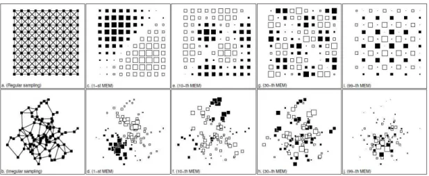
(MEM) for a model enables one to observe spatial relationship with results (Figure 8). The more positive eigenvector values are, the more spatial phenomena is evident [46].

Figure 8: MEM for regular (up) and irregular (bottom) network – first in a tow have positive and last in a row have negative eigenvector values. Derived from [46]

2.3.7

Model selection

In statistical investigation it is always a concern as to whether one model is better than other. The choice for the best model requires some model selection criteria. Every model contains a

score or value on which we can be based quality. Therefore the candidate which better scores should be chosen for further analysis [47].

In this analysis, the model selection is based onto further selection steps:

 Model selection in regards to the most suitable variables for both GLM and GAM  Model selection in regards to the best GLM

 Model selection in regards to the best GAM

 Model selection in regards to the best ultimate model

The most popular methods for model selection are as follows:  Akaike Information Criterion (AIC)

 Bayesian Information Criterion (BIC)

In the literature authors do not state a significant difference between them, however generally

AIC finds the model which gives the best prediction, while BIC selects model which is considered as a “true” model [48].

Both AIC and BIC are based on maximum likelihood parameter estimates. AIC is defined to be -2 multiplied with log-likelihood with addition of 2 multiplied with number of parameters:

𝐴𝐼𝐶 = −2𝑙𝑜𝑔𝑙𝑖𝑘 + 2𝑑 (12)

Unlike AIC, BIC model selection is defined as:

𝐵𝐼𝐶 = −2𝑙𝑜𝑔𝑙𝑖𝑘 + log(𝑛)𝑑 (13)

N is number of observations. Thus, from equations BIC penalizes parameters more than AIC.

number of covariates. In the project analysis the idea was to have as minimum as possible variables in order to have a more robust model and more secure variables throughout. The workflow of the model selection criteria is based on BIC [49], although for the neighbourhood

criteria between city sections, it is based on AICc criteria. AICc is an AIC model, however for the confined sample size. The assumption for the AICc is that the model has to follow normal

distribution for residuals that is linear, hence the formulation is:

𝐴𝐼𝐶𝑐 = 𝐴𝐼𝐶 +2𝑑(𝑑+1)_{𝑛−𝑑−1}

(14)

According to the formula it is more robust and penalizes parameters slightly higher than AIC. For the comparison of several models, an analysis of variance (ANOVA) is computed. ANOVA

provides an efficient analysis of variance in a sequential order. It compares the smaller model (with fewer variables) against the next in the sequence that is a more complex model with at least one more variable. The comparison step is examined with likelihood ration test. The output

contains residual degrees of freedom and deviance from each model. For the models with a given dispersion which is Poisson, the chi-squared test is recommended [50].

The p- value tests the null hypothesis that groups of all populations have the identical mean. It means if p-value is large, then there is not enough evidence that means are different. So, the

population means are all equal, thus we do not have enough evidence to reject null hypothesis. If p-value is smaller than 0.05, then we reject null hypothesis saying that there is statistical

evidence to prove that all populations have identical means.

2.3.8

Predictive approaches - related applications

The flow for the predictive modelling is partially derived from papers related to rat sightings

[51] and residential burglaries [52], and it is rearranged together for the purpose of this study. Furthermore, in proposed approach both GLM and GAM are taken into account. In the first

paper [51] authors decided to find the association between aggregated observations per census track and the predefined focus points. In fact, they proved that association exists and that

distance model is the most appropriate model. The model discovers even unexpected results such as that cat’s feeding stations are attractive to rats. So, the distance model was better than other models and this was used for further analysis to find out indicators that have associations with focus areas. The approach related to the distance can be implemented in our example since

focus areas can be established, but the other issue is lack of data in terms of factors for restaurants potentiality. On the other hand, an aim is to globally evaluate city sections; however

shopping malls, or the most popular tourist sites, and radius with influence factors can be established accordingly, but it will remain open for some future studies.

The second paper [52] presents an innovative approach for crime probability prediction with

the assistance of cut-offs based on fractal skill score. Non-linearity in the covariates shares the common behaviour with covariates from our study. A one-dimensional smoother is

implemented for continuous predictors and two-dimensional isotropic smoother is applied for spatial component in GAM. In addition their approach is in a way improved with temporal

component, i.e. with three dimensional smoother, however our method is static, hence is not necessary.

One of the alternatives to consider is zero inflated model. A zero inflated regression model addresses with existence of zero events in response variable. In Lisbon, many city sections do

not have restaurants. That would indicate that zero inflated Poisson (ZIP) distribution could be implemented. However it is important to differentiate structural zeros within population.

Structural zeros are associated for those subgroups which can be identified from the population that have no risk at all to change behaviour. In contrast, there are random zeros or sampling

zeros, which are produced by sampling variability [53]. An assumption is that certain subgroups from the population will never change behaviour, in other words they would always have associated zero counts. It can be a good idea to test for the future work, however in this research

structural zeros are not considered. In this study every neighbourhood is regarded that has some degree of potentiality for restaurants either negatively or positively.

Regarding GLM model, since Moran’s I test is a mean for detecting spatial autocorrelation, in the same way it can be utilized for embedding spatial autocorrelation into a model. In this sense,

Moran eigenvector calculates two eigenvectors from the spatial lag of GLM model with spatial weights and afterwards it is fitted into the full GLM model [42].

Following theoretical framework it can be noted the importance of involving a spatial

dimension both in segmentation and prediction map. SOM in many examples proved that it can be good method to cluster census data, however the novel step was to test significance of

3

STUDY AREA

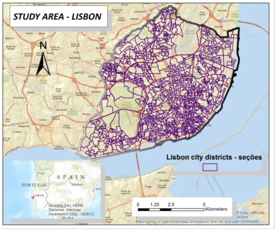
Lisbon is the capital and simultaneously the largest city of Portugal. The municipality of Lisbon (Portuguese: concelho) has approximately half a million people [54]. The municipality is

divided into 24 districts (Portuguese: frequências) or small 1054 sections (Portuguese: seções). It is even further divided into smaller areas called sub-sections. For the purpose of the thesis,

the level of detail selected is at a city section scale, although it is recommended as smallest as possible. However the sub-sections in terms of privacy concerns have limited a number of variables, so the city section level of detail has been chosen. On Figure 9 some sections are very

small and other very large, hence the size and borders of the sections does not follow a set standard areal extent. In general, downtown areas such as Estrela, Santa Maria Maior, Santo

Antonio and Misericordia usually have smaller sections, dense populations and are located on the south east of the map. Other city-sections such as Ajuda, Benfica, Olivais, Belem, have

mainly larger or moderate size sections and surround the downtown area.

Figure 9: Study area – Lisbon

Sections of the city vary in elevation. In downtown, older areas along the water edges have lower elevation, while surrounding sections are higher. The landscape of Lisbon contains slopes

ranging from small rolling hills that are widely distributed along the Tagus River to the peaks of Sintra Mountains. Thus, there are many sightseeing points towards downtown and the river

4

METHODOLOGY

In general, the proposed structural framework at Figure 102 _{contains three parallel processes,}

which are dependent on each other. The final step combines the visualization process and it

obtains an overall visualization.

The first step was to combine EDA and ESDA analysis in order to obtain an interpretation of variables. The second parallel process was SOM implementation with socio-demographic

components provided by census data. The objective is to derive clusters which could lead to better analysis of potentiality of restaurants. Next step is the prediction of the restaurants

according to the best selected models. Later on, it is important to specify cut-offs from deviance residuals and undertake classification according to potentiality.

2 _{Legend for flowcharts refer to ANNEX 1}

DATASET DESCRIPTIVE STATISTICS EXPLORATORY ANALYSIS END: ArcGIS *.SHP SELF ORGANIZED MAPS PROCESS SELF-ORGANIZED MAPS Input parameters Choropleth map

GLM BASE MODEL GAM BASE MODEL

PREDICTIVE MODELING

 Dataset: 80% for training and 20% testing

SPATIAL GAM SPATIAL GLM NEIGHBORHOOD CRITERIA BEST MODEL SELECTION BEST MODEL EMPIRICAL TEST FOR BELL-SHAPED APPROXIMATION *.SHP *.SHP

4.1

Dataset

The National Statistical Institute of Portugal provides 122 variables on the level of city section from the census 2011. Data can be divided into the following categories:

 Related to buildings (type, functionality, date of building…)  Accommodation

 Households  Individuals  Education

Selected variables for the purposes of the study are presented in Table 1.3

Chosen variables Code

1 Private households with 1 or 2 people Hous1or2

2 Private households with 3 or 4 people Hous3or4

3 Private households with no unemployed HousNoUnem

4 Resident individuals aged 20 to 24 years Indv20_24

5 Resident individuals aged 25 to 64 years Indv25_64

6 Men residents aged 20 to 24 years Men_20_24

7 _{Men residents aged between 25 and 64 years} Men_25_64

8 Women residents aged 20 to 24 years Womn_20_24

9 _{Women residents aged between 25 and 64 years} Womn_25_54

10 Men residents aged more than 64 years Men_64_

11 Women residents aged more than 64 years Woman_64_

12 Individuals’ residents with post-secondary education Post_sec_e

13 Resident individuals with a college degree Colle_deg

14 Pensioners or retired individuals living Pensions

15 Resident individuals without economic activity Res_No_act

16 Exclusively residential areas Exlus_res

17 Employed individuals resident in the secondary sector Work_Sec

18 Resident Individuals employed in the tertiary sector Work_in_Ter

19 Individuals employed residents Employed

20 Buildings constructed from 2001 BuildAft01

Table 1: Selected variables from Census 2011

The variable Tax_index4 is used to represent an economic indicator in terms of wealth for each city section. It was taken over from Portuguese Tributary and Customs Authority (Portuguese:

AT Autoridade Tributaria e Aduaneira).

The number of tourist sites - Tourst_idx presents count per city section. Since the coordinates are known for every location, the total number per site is calculated according to spatial

summary. The chosen attributes that present Tourist index are presented in Table 2. The total number of tourist sites in Lisbon, have 720 records for the year 2015.

Selected sites - Totals Historical monuments Airport

Casino Ferry terminal Hotel

Museum

Rental car agency Taxi stand Tourist attraction Tourist information Winery shop

Table 2: Tourists sites – totals

In terms of restaurants, they were determined on the same way as tourist sites. Likewise,

Restaurant variable indicates a number of restaurants per city section. Both X and Y locations

of tourist sites and restaurants are provided from Here Maps with assistance from the official

Here maps office in Lisbon.

Consequently, the final dataset presents the variables from Table 1, Tax_index, Tourist_idx, Restaurant arranged by city sections, thus they are stored into shapefile (including supporting

files such as: *.dbf, *.shx, *.cpg, *.shp.xml, *.sbx, *.sbn).

4.1.1

Data pre-processing

The raw data file for restaurants and tourist sites contained many redundancies. Therefore the

procedures in R were conducted to erase them. Many items were previously converted from polygons to number of points and thus one restaurant would be represented four times in

dataset. We required that one restaurant represent one count in order to achieve the number of restaurants within a certain city section.

The second issue was projection; reference system or simply coordinate system. The data from

Here Maps was in WGS-84 longitude and latitude coordinate system. However the provided

dataset from census data was in local Portuguese reference system ETRS_1989_TM06-Portugal. Therefore restaurants and tourist sites were converted to the local Portuguese system

4.1.2

Data normalization

In the study area, some city sections are more populated than others and varied in size. Therefore all of them have to be categorized on the same scale.

Firstly, the variables related to population were calculated in terms of percentage per unit, as well as number of buildings. On the other hand, it was not appropriate to calculate percentage

counts from restaurants and tourist sites, therefore within combined dataset from all variables

Min-Max normalization was applied.

Normalization is a process where the values from variables are approximated on a common

scale. There are many methods, however Min-Max summarizes values in a range [0, 1] [55]. The normalization is necessary for SOM and it is computed using the following equation:

𝑀𝑀 = _{𝑚𝑎𝑥−𝑚𝑖𝑛}(𝑥−𝑚𝑖𝑛) (15)

Where:

x– field value

min– minimal value in an array

max– maximal value in an array

4.1.3

Analysis Approach

The approach taken for this project included a series of tests and evaluations in order to decide

on the best methods to be applied for all aspects of this project.

In terms of the descriptive statistics, the methodology is presented as shown in Figure 11.

Figure 11: Descriptive statistics

DATASET

Restaurant Tourist

sites Census

data

DESCRIPTIVE STATISTICS

HISTOGRA

PARALLEL COORD. BOXPLOT

*.SHP

EXPLANATORY ANALYSIS

ArcGIS *.SHP

In the previous section a shapefile was made and a number of graphs and plots were created in order to recognize patterns (both obvious and hidden).

It is important to have a general picture about the most important variables i.e. restaurants and

tourist sites in Lisbon in order to perform further detailed analysis. For this purpose a geographic map with layers of restaurants and tourist sites was created.

It is important to find clusters that are most suitable for restaurants and to provide an explanatory spatial data analysis from socio-demographic clusters. In addition, for SOM

geographical index is added so that clusters are assigned to city sections. The workflow is presented in Figure 12. In the first step it is necessary to specify input parameters from a previously normalized dataset. In the process step, from output graphs we measure quality of

SOM. An important part is to analyze graphs from component planes as well as distance matrix. Vector of mean deviations helps to identify how distant are deviations from code vectors. Along

with iterations the deviance is decreasing. In order to uphold more automatic decision, within SOM process, k-means and hierarchical clustering are executed in order to determine number

of clusters.

SELF ORGANIZED MAPS PROCESS

Hierarchical clustering

SELF-ORGANIZED MAPS

GRID SIZE

TOROIDAL

Learning Unit

Neuron shape

Variable selection

Vector of mean

deviation Component

planes

U—matrix

Matrix of Quality

K-means

By ID

Choropleth map

Descriptive statistics for clusters

ArcGIS

*.SHP

To enhance visualization and improve data analysis the decision was made to divide the dataset and develop several SOMs. The initial representatives as an input matrix are chosen from data, thus all SOMs have mutual start matrix of positions. Selected variables for each SOM are

presented in Table 3.

SOM_entry SOM_mixed SOM_population SOM_household

Individuals 20-24 Household 1 or 2 Individuals 25-64

Household with 1

or 2

College educated Active Population College educated Active population

Residence with no

activity Post-secondary education Work in tertiary Individuals 20-24

Work in tertiary College education Work in secondary

Residence with no activity

Tax value Residence with no activity Tax value Residence 20-64

Tourist index Work in tertiary Tourist index Work in tertiary

Men 25-64 Tax value Woman 25-64 Tax value

Women 25-64 Tourist index Woman 64 Tourist index

Women 64 Women 64 Men 64 Employed

Men 64 Men 64 Pensioners

Building built after 2001

Buildings built after

2001 Pensioners Employed

Exclusively

residential

Exclusively

residential Employed

Household with 3 or 4 Exclusively residential Household 3 or 4

Table 3: Selected variables for each SOM model

A detailed flowchart is presented in Figure 13.

Figure 13: Flowchart - Predictive modelling

In the first step for the purpose of verifying, the dataset is divided for training 80% and testing 20%. The polygons were selected according to the systematic selection, i.e. in the sequence

every fourth polygon or city section were selected for testing sample, instead of having random samples. The 20% of test data is left for the model evaluation at the end, with 80% for model

construction. GLM BASE GAM BASE PREDICTIVE MODELING *.SHP Systematic selection 20% for testing

80% - training for model construction

Response: Restaurant

Family: Poisson

Link function: log

Parameters: IRLS

Model selection:

Stepwise: forward/back

Criterion: BIC

GAM SPATIAL GLM SPATIAL

NEIGHBOURHOOD CRITERIA Spatial weights Spatial autocorrelation test

Family: Poisson

Link function: log

Parameters: REML

Model selection:

Stepwise: forward

Criterion: BIC

Centroids of neighbour

hoods

BEST MODEL SELECTION ANOVA test

Prediction for 20% test

RMSE, BIC

4.1.4

Base model construction

Restaurants variable has a count per city section, therefore it belongs to the Poisson discrete link function. In other words the output belongs to a family of natural asymmetric numbers.

The link function for the mean approximation is logarithmic. While base GLM and GAM were created using Poissonloglink function, the parameters were estimated with REML for GAM

and IRLS for GLM. The components for the construction of the GLM are as follows:  Based on formula (1) :

a. q(µ)– response variable - Restaurants

b. βk - estimated parameters based on IRLS c. xk - covariates – all other variables  Link function from (3)

 Poisson: Discrete – {0}U N – Count - Asymmetric

In order to determine what is suitable the starting model is assigned for full model. The full model contains the whole set of covariates.

So, the complete GLM is presented with the following covariates:

 BuildAft01, Colle_deg, Employed, Exlus_resi , Hous1or2, Hous3or4, HousNoUnem,

Men_20_24, Men_25_64, Men_64_, Pensioners, Res_No_act, Tax_index, Tourst_idx, Woman_64_ , Womn_20_24, Womn_25_64, Work_in_Te, Work_Sec

Having applied GLM, as an output it is possible to extract deviances residuals, estimated coefficients, standard deviation, z value as well as probability value – p value.

 Ho hypothesis explains that covariate is meaningful as a predictor if p– value≤ 0.  In contrary, if p-value > 0.05, covariate should be rejected.

From the complete GLM model there are important covariates: buildings after 2001,

exclusively residential areas, men aged between 20-24, tax, tourist sites and women above the age of 64.

In contrast, covariates such as working in secondary or tertiary sector, pensioners, employed

etc. were not presented significant contribution for prediction. In the further step a

backward/forward stepwise selection method was applied.

Covariate selection was established via Bayesian information criterion (BIC) described in

Model Selection section. BIC value is based on:  the observed data,

 parameters of model,  the number of observations,

 the number of estimated parameters and  likelihood function

From all possible combinations of covariates and completed GLMs, according to BIC criterion, the selected model produces the base GLM with following covariates ordered by importance:

𝑙𝑜𝑔(µ) = 𝛽𝐼+ 𝛽1𝑇𝑜𝑢𝑟𝑖𝑛𝑑𝑒𝑥+ 𝛽2𝑇𝑎𝑥𝐼𝑛𝑑𝑒𝑥+ 𝛽3𝐻𝑜𝑢𝑠3𝑜𝑟4+ 𝛽4𝐸𝑥𝑙𝑢𝑠𝑖𝑟𝑒𝑠𝑖𝑑+ 𝛽5𝑀𝑒𝑛2564

+𝛽6𝑊𝑜𝑚𝑎𝑛64 + 𝛽7𝐴𝑐𝑡𝑖𝑣𝑒 (16)

Tourst_idx, Tax_index, Hous3or4, Exlus_resi, Men_25_64, Woman_64_, HousNoUnem

One of the objectives of the thesis is to identify the city sections potentially for restaurants,

hence we propose the method to calculate the deviance of the residuals between predicted and existing number of restaurants in order to determine thresholds values for cut-offs. In the

flowchart (Figure 14), the first step is to derive the formula from the best selected model. However, since the best selected model contains 80% of training data, the formula is extracted

and applied for the whole dataset. In the second step deviance residuals are calculated. Finally, the threshold for cut-offs are defined according to empirical test for bell-shaped approximation.

BEST SELECTED MODEL

Formula

EMPIRICAL TEST FOR BELL-SHAPED APPROXIMATION

Restaurant prediction Deviance

residuals *.SHP

ArcGIS online Map with

layers

 No change (µ ± SD)

 Over/underestimated( 2 SD ± SD)

 Extreme (±2 SD)

5

RESULTS AND ANALYSIS

In descriptive statistics one of the steps is to present visual interpretation of the variables

particularly characterized with spatial features.

In Figure 15 hotspots of tourist attractions is overlapped with restaurants. In Figure 16 a density

map of restaurants with tourist sites is shown. It is visually clear that downtown areas contain higher values from both (usually around shopping malls, and trade markets) restaurants and

tourist sites. However, there are locations where this patterns is not always respected. In that regard further analysis will reveal the most influential combination of variables to achieve this.

Regardless, the sites where there are restaurants and non-touristic sites are important for prediction, as well.

Figure 16: Density of restaurants

The larger areas where tourist sites are located without restaurants are mainly large green parks

detected from imagery. With regards to non-tourist sites, the presence of restaurants identified from imagery are mainly markets and city sections on longer distance from tourist sites. One

could infer, that restaurants are creating something similar to buffer zones around tourist sites. The conclusion from images is that tourist sites and restaurants in general are spatially correlated, however the important outliers could be visually identified.