Automation of a reactor for enzymatic hydrolysis of sugar cane bagasse: Computational intelligence-based adaptive control

Federal University of São Carlos Graduate Program in Chemical Engineering

Master Thesis

Automation of a reactor for enzymatic

hydrolysis of sugar cane bagasse:

Computational intelligence-based adaptive

control

Vitor Badiale Furlong

Advisor: Prof. Roberto de Campos Giordano Coadvisor: Prof. Marcelo Perencin de Arruda Ribeiro

Vitor Badiale Furlong

Automation of a reactor for enzymatic

hydrolysis of sugar cane bagasse:

Computational intelligence-based adaptive

control

Master thesis submitted to the Graduate Program in Chemical Engineering, Center of Exact Sciences and Technology, Federal University of São Carlos, as partial fulfillment of the requirements for degree of Master of Science.

Advisor: Prof. Roberto de Campos Giordano

Ficha catalográfica elaborada pelo DePT da Biblioteca Comunitária UFSCar Processamento Técnico

com os dados fornecidos pelo(a) autor(a)

F985a Furlong, Vitor Badiale Automation of a reactor for enzymatic hydrolysis of sugar cane bagasse : Computational intelligence-based adaptive control / Vitor Badiale Furlong. --São Carlos : UFSCar, 2016.

65 p.

Dissertação (Mestrado) -- Universidade Federal de São Carlos, 2015.

To my parents.

In retribution to all the love and care.

AGRADECIMENTO – ANP

Agradecimentos Pessoais

Aos Professores Roberto e Marcelo pela dedicação. A banca examinadora, pela disponibilidade.

A minha família, pelo amor e paciência.

A Fabiane Cristina, pelo amor e por aguentar a minha falta de paciência.

Aos colegas de laboratório, atuais e antigos, amigos e todos aqueles que tem que aguentar o meu mau humor diariamente.

There are two types of people in the world:

-Those who can extrapolate from incomplete data.

ABSTRACT

The continuous demand growth for liquid fuels, alongside with the decrease of fossil oil reserves, unavoidable in the long term, induces investigations for new energy sources. A possible alternative is the use of bioethanol, produced by renewable resources such as sugarcane bagasse. Two thirds of the cultivated sugarcane biomass are sugarcane bagasse and leaves, not fermentable when the current, first-generation (1G) process is used. A great interest has been given to techniques capable of utilizing the carbohydrates from this material. Among them, production of second generation (2G) ethanol is a possible alternative. 2G ethanol requires two additional operations: a pretreatment and a hydrolysis stage. Regarding the hydrolysis, the dominant technical solution has been based on the use of enzymatic complexes to hydrolyze the lignocellulosic substrate. To ensure the feasibility of the process, a high final concentration of glucose after the enzymatic hydrolysis is desirable. To achieve this objective, a high solid consistency in the reactor is necessary. However, a high load of solids generates a series of operational difficulties within the reactor. This is a crucial bottleneck of the 2G process. A possible solution is using a fed-batch process, with feeding profiles of enzymes and substrate that enhance the process yield and productivity. The main objective of this work was to implement and test a system to infer online concentrations of fermentable carbohydrates in the reactive system, and to optimize the feeding strategy of substrate and/or enzymatic complex, according to a model-based control strategy. Batch and fed-batch experiments were conducted in order to test the adherence of four simplified kinetic models. The model with best adherence to the experimental data (a modified Michaelis-Mentem model with inhibition by the product) was used to train an Artificial Neural Network (ANN) as a softsensor to predict glucose concentrations. Further, this ANN may be used in a closed-loop control strategy. A feeding profile optimizer was implemented, based on the optimal control approach. The ANN was capable of inferring the product concentration from the available data with good adherence (Determination Coefficient of 0.972). The optimization algorithm generated profiles that increased a process performance index while maintaining operational levels within the reactor, reaching glucose concentrations close to those utilized in current first generation technology a (ranging between 156.0 g.L ¹ and 168.3⁻ g.L ¹). However rough estimates for scaling up the reactor to industrial dimensions⁻ indicate that this conventional reactor design must be replaced by a two-stage reactor, to minimize the volume of liquid to be stirred.

RESUMO

A crescente demanda por combustíveis líquidos, bem como a diminuição das reservas de petróleo, inevitáveis a longo prazo, induzem pesquisas por novas fontes de energia. Uma possível solução é o uso do bioetanol, produzido de resíduos, como o bagaço de cana-de-açúcar. Dois terços da biomassa cultivada são bagaço e folhas. Estas frações não são fermentescíveis quando se usa a tecnologia de primeira geração atual (1G). Um grande interesse vem sendo prestado a técnicas capazes de utilizar os carboidratos deste material. Dentre elas, a produção de etanol de segunda geração (2G) é uma possível alternativa. Etanol 2G requer duas operações adicionais: etapas de pré-tratamento e hidrólise. Considerando a hidrólise, a técnica dominante tem sido a utilização de complexos enzimáticos para hidrolisar o substrato lignocelulósico. Para assegurar a viabilidade do processo, uma alta concentração final de glicose é necessária ao final do processo. Para atingir esse objetivo, uma alta concentração de sólidos no reator é necessária. No entanto, uma carga grande de sólidos gera uma série de dificuldades operacionais para o processo. Este é um gargalo crucial do processo 2G. Uma possível solução é utilizar um processo de batelada alimentada, com perfis de alimentação de enzima e substrato para aumentar produtividade e rendimento. O principal objetivo deste trabalho é implementar e testar um sistema para inferir concentração de carboidratos fermentescíveis automaticamente e otimizar a política de substrato e/ou enzima em tempo real, de acordo com uma estratégia de controle baseada em modelo cinético. Experimentos de batelada e batelada alimentada foram realizados a fim de testar a aderência de 4 modelos cinéticos simplificados. O modelo com melhor aderência aos dados experimentais (um modelo de Michaelis-Mentem modificado com inibição por produto) foi utilizado para gerar dados a fim de treinar uma rede neural artificial para predizer concentrações de glicose automaticamente. Em estudos futuros, esta rede pode ser utilizada para compor o fechamento da malha de controle. Um otimizador de perfil de alimentação foi implementado, este foi baseado em uma abordagem de controle ótimo. A rede neural foi capaz de predizer a concentração de produto com os dados disponíveis de maneira satisfatória (Coeficiente de Determinação de 0.972). O algoritmo de otimização gerou perfis que aumentaram a performance do processo enquanto manteve as condições da hidrólise dentro de níveis operacionais, e gerou concentrações de glicose próximas as obtidas pelo caldo de cana-de-açúcar da primeira geração (valores entre 156.0 g.L ¹ e 168.3 g.L ¹). No entanto, estimativas iniciais de aumento de escala do⁻ ⁻ processo demonstraram que para atingir dimensões industriais o projeto do reator utilizado deve ser analisado, substituindo o mesmo por um processo em dois estágios para diminuir o volume do reator e energia para agitação.

FIGURES INDEX

Figure 1 – Lignocellulosic Biomass Processing...4

Figure 2 - Monitoring and control system...20

Figure 3 - Sensor array coupling... 21

Figure 4 - Interpolation Example... 25

Figure 5 - Model Fitting Flowchart... 29

Figure 6 - Feeding profile optimization...31

Figure 7 – Cross Validation Procedure... 33

Figure 8 - Evaluated transfer functions...34

Figure 9 - Training and Validation Data set Error...34

Figure 10 - Conductance and glucose concentration during hydrolysis...35

Figure 11 - Full Array Monitoring During Batch Experiments...36

Figure 12 - Full Array Monitoring During Fed-batch Experiments...36

Figure 13 – Supernatant Scans During Fed-batch Experiments...37

Figure 14 – Supernatant Scans from 250 to 320 nm...37

Figure 15 – Experimental Data for Batch Experiments...38

Figure 16 – Experimental Data for Fed-batch Experiments...39

Figure 17 – Batch Experiments Co-products Linear Fitting...39

Figure 18 – Batch Experiments Co-products Linear Fitting...40

Figure 19 - Model fitting for Batch Experiments...41

Figure 20 – Model Fitting for Fed-batch Experiments...41

Figure 21 – Confidence Region for the Modified MM Model with Product Inhibition...43

Figure 22 – Stirring Power/Solids Concentration Scatter Plot...44

Figure 23 – Solids Above 97 g.L⁻¹ Region Exponential Fitting...45

Figure 24 – Solids Bellow 97 g.L⁻¹ Region Exponential Fitting...45

Figure 25 – Fed-batch Optimization for 360 h Process...47

Figure 26 – Fed-batch Optimization for 360 h Process Without Stirring Power...50

Figure 27 – Fed-batch Optimization for 360 h Process With Feeding Restriction...51

Figure 28 – Artificial Neural Network Errors – Poslin and Logsig Architectures...53

Figure 29 – Artificial Neural Network Errors – Poslin and Logsig Architectures...54

TABLE INDEX

Table 1 – Typical Composition of Sugarcane Bagasse Before and After Autohydrolysis.. 5

Table 2 – Classification of Cellulose Hydrolysis Kinetic Models...7

Table 3 – Enzymatic Fed-Batch Hydrolysis of Lignocellulosic Biomass...12

Table 4 – Fed-Batch Feeding Profile... 19

Table 5 - Particle Swarm Optimization Pseudocode...27

Table 6 – Co-products Linear Fitting... 40

Table 7 – Models Parameters with 95% confidence intervals...42

Table 8 – Correlation Table for the Modified MM Model with Product Inhibition...42

Table 9 – Stirring Power Fitting Models...46

Table 10 – Unrestricted Feeding Policy...46

Table 11 – Unrestricted Feeding Policy Without Stirring Cost...49

ABBREVIATIONS AND ACRONYMS INDEX

1G – First Generation 2G – Second Generation ANN – Artificial Neural Network

CSS – Conductance and Capacitance Spectroscopy FPU – Filter Paper Units

gbest – Global Best

LPS – Least Partial Square MLP – Multilayer Perceptrons MM – Michaelis-Mentem MO - Modified

NF – Neuro-Fuzzy NN – Neural Network

ODE – Ordinary Deferential Equation PCA – Principal Component Analysis PH – Pseudo-Homogeneous

PI – Product Inhibited pbest – Personal Best

PSO – Particle Swarm Optimization USB – Universal Serial Bus

SUMARY

Abstract... v

Resumo... vi

Figures Index... vii

Table Index... viii

Abbreviations and Acronyms Index... ix

1. Introduction And Objectives... 1

2. Literature Review... 3

2.1. Lignocellulosic compounds... 3

2.2. Biomass Pretreatment... 4

2.3. Lignocellulosic Biomass Hydrolysis...5

2.4. High Solids Enzymatic Hydrolysis...9

2.5. Biomass Hydrolysis in semi-continuous Operations...10

2.6. Optimal Control... 12

2.7. Enzymatic Hydrolysis Fed-Batch Optimal Control...13

2.8. Online Fermentable carbohydrates Determination...15

3. Materials and Methods... 18

3.1. Enzymatic Hydrolysis... 18

3.2. Monitoring and Control System...19

3.3. Experimental Apparatus... 20

3.4. Carbohydrates Determination... 23

3.5. Model Fitting... 24

3.6. Fed-Batch Optimization... 29

3.7. Neural Network Optimization... 32

4. Results and Discussion... 35

4.1. Conductivity Monitoring... 35

4.2. Full Array instrumentation... 35

4.3. Batch and Fed-batch Experimental Data...38

4.4. Parameters Fitting... 40

4.5. Stirring power/Solids Relation... 44

4.6. Feeding Profile Optimization... 46

4.7. Neural Network Calibration... 52

5. Conclusions... 57

6. Further Studies Suggestions... 58

1. INTRODUCTION AND OBJECTIVES

The continuous demand growth for liquid fuels, alongside with the decrease of fossil oil reserves, unavoidable in the long term, induces investigations for new energy sources. A possible solution to substitute some liquid fossil fuels is the use of bioethanol, produced from renewable sources (NAIK et al., 2010).

In Brazil, a massive production of ethanol as automotive fuel occurred in the 1970s, when the government initiated a national program (Pró-Álcool) to reduce the dependency on foreign refined oil. The Pró-Álcool program had as main starting material sugarcane juice. This culture was intensified during this period, especially in southeast Brazil. The technology used in the program, called first generation (1G), was similar to the one utilized nowadays. But two thirds of the cultivated biomass, i.e. sugarcane bagasse or other lignocellulosic materials such as leaves, generates non fermentable substrates when the current process is applied (FREITAS & KANEKO, 2012).

Even though the biomass that is non fermentable via 1G processes may be used to generate other forms of energy (bioelectricity, production of syngas and so on), there is great interest in developing techniques capable of converting the carbohydrates from this material into bioethanol, thus generating more ethanol from each sugarcane mass unit (DANTAS et al., 2013).

Currently, large-scale 2G ethanol production still presents economic bottlenecks, . Among the most important technical hindrances is the scale up of the hydrolysis process to industrial application, in order to generate high product yields while keeping costs low (MODENBACH & NOKES, 2013).

This work intended to test and implement a softsensor architecture using Artificial Neural Networks, to predict the concentration of sugars in a bioreactor during the enzymatic hydrolysis of pretreated sugarcane bagasse using cellulases from a commercial cocktail. Besides, an algorithm based on optimal control theory was implemented, to define feeding strategies of substrate and/or enzymatic complex for the hydrolysis reactor.

final results hardly could be applied, directly, to industry-scale reactors.

2. LITERATURE REVIEW

2.1. LIGNOCELLULOSIC COMPOUNDS

Second generation biofuels are fuels produced from lignocellulosic substrates. These are fibers found in plants and vegetables. Their main function is to provide structural support, while assuring microbiological and chemical protection. The fractions of lignocellulosic materials are mostly composed by cellulose (32–55%), hemicellulose (19– 24%), lignin (23–32%) and ashes (3–6%) (SANTOS et al., 2012).

Cellulose (C6H1005)n is the most abundant polysaccharide in the fiber. Its ordered

structure consists of several hundred glucose molecules (XU et al., 2013). The cellulose spatial conformation is determined by three main interactions. The first interaction is the

β→1,4 glycosidic bond that unites a glucose to another glucose molecule through a covalent bond. This generates cellobiose, and this disaccharide is repeated throughout the polymer chain (ROCHA et al., 2011). The second interaction is among hydrogen molecules from the same chain and the third between adjacent chains. Due to these interactions, part of cellulose macromolecules can form a crystalline region, granting to the entire structure a high cohesiveness, and rendering it insoluble in water and several other solvents, and resistant to hydrolysis (SANTOS et al., 2012).

Hemicellulose differs significantly from cellulose. It is a heteropolysaccharide composed by hexoses (glucose, galactose and mannose), pentoses (xylose, the most abundant monomer, and arabinose), acetic acid, glucuronic acid and 4-O-methy-glucuronic acid. The relation between these substances differs from vegetable to vegetable. This portion of the tissue does not form crystalline regions, thus it can be removed or hydrolyzed more easily than cellulose (CANILHA et al., 2012).

Lignin is formed by the polymerization of p-coumaryl alcohol, sinapyl alcohol and coniferyl alcohol. It is the second most abundant polymerer in the lignocellulosic biomass, and provides a barrier against foreign agents. Recalcitrance of the biomass is in great part due to this lignin barrier (ARANTES & SADDLER, 2011). In order to prevent this effect, a delignification procedure may be applied. From a biorefinery point of view, the recuperated lignin may be used in other processes (STEWART, 2008). Alternatively, its combustion will provide an extra heat source to the 2G process.

polysaccharides must be hydrolyzed, so that their monosaccharides (mostly pentoses and hexoses) become available to fermentative microorganisms. However, before the hydrolysis process, a pretreatment is required to separate and render cellulose and hemicellulose available to the hydrolytic action of the enzyme cocktail. A representation of the process is in Figure 1.

Figure 1 – Lignocellulosic Biomass Processing

(Source: author’s collection, adapted from: SANTOS et al., 2012) 2.2. BIOMASS PRETREATMENT

The pretreatment procedure destabilizes the lignocellulosic structure, making it more susceptible to further processing. This is achieved by increasing the material porosity, reducing cellulose crystallinity and removing lignin, to a certain degree. The entire procedure must be applied up to an intensity that generates an optimum platform for subsequent operations, while considering the formation of inhibitors and cost effectiveness (CHIARAMONTI et al, 2012).

Several methodologies are available for this process. Thus, the choice of the most adequate pretreatment depends on the feedstock, process plant design and economic situation (BANERJEE et al., 2010).

pressurized reactor to maintain water in a liquid state at temperatures ranging from 150ºC to 230ºC, for different time periods. At these temperatures, biomass suffers cooking, increasing cellulose digestibility, while producing small amounts of inhibitors (KIM et al., 2009).

Another advantage of this technology is the absence of additional chemical compounds during the process, yielding a less toxic effluent than other alternatives. However, this pretreatment does not alters lignin to an extent that may render these molecules inactive in subsequent processes (MENON & RAO, 2012). A typical composition of sugarcane bagasse, for the most significant compounds, before and after the autohydrolysis process is presented in Table 1.

Table 1 – Typical Composition of Sugarcane Bagasse Before and After Autohydrolysis. Compound Raw Sugarcane Bagasse Autohydrolysis Treated

Bagasse Cellulose

(% w.w ¹)⁻ 38.0 54.3

Hemicellulose

(% w.w ¹)⁻ 29.4 5.9

Lignin

(% w.w ¹)⁻ 21.7 24.8

(Source: Adapted from RODRIGUEZ-ZÚÑIGA et al., 2014) 2.3. LIGNOCELLULOSIC BIOMASS HYDROLYSIS

The pretreated biomass must be further hydrolyzed to provide fermentable fractions. At this stage, the polymers released by the pretreatment are converted to free monomers, readily available to fermentation. Two mains technologies are used in order to hydrolyze lignocellulosic materials, using acid solution, generally sulfuric acid, or using enzymatic complexes (GAMAGE et al., 2010; SUN & CHENG, 2002).

Acid hydrolysis is usually divided in two groups, diluted and concentrated acid hydrolysis. In diluted acid hydrolysis, acid concentrations range from 1 to 3% w.w-1_{, at high}

Concentrated acid is a more common process methodology. In this operation the acid concentration is high (90% w.w-1_{) and, therefore, temperatures can be lower. Thus,}

this process generates a smaller amount of inhibitors. However, the utilization of such high acid concentrations is costly, and also generates a highly toxic effluent (SUN & CHENG, 2002).

This leads to the necessity for a more economically and environmental suitable process. One alternative is enzymatic hydrolysis. This sort of procedure yields high conversions, with fewer risks of producing toxic secondary products (LIMAYEM & RICKE, 2012). However, a high cost is inherent to this process, since, the compound itself has a high value and, with the current technology, direct enzymatic complex reuse is not feasible when using a soluble enzymatic complex (DANTAS et al., 2013).

To introduce enzymatic hydrolysis into the ethanol production route several research fronts are explored, among them: enzymatic complex improvement (KUPSKI et al., 2013); implementations of the second generation technology alongside the first generation process (FURLAN et al., 2012); utilizing high substrate loading; hydrolysis optimization modifying the feeding policy to the reactor in a fed-batch process (HODGE et al., 2009; CAVALCANTI-MONTAÑO et al., 2013).

2.3.1. Modeling Enzymatic Lignocellulosic Biomass Hydrolysis

To optimize the bioreactor design and operational conditions it is necessary to understand the kinetics that commands the interaction of the lignocellulosic material and the enzymatic complex. This study is difficult since several effects are reported among substrate and catalyst (SOUSA JR et al., 2011). To cope with such complexity, a large number of models are proposed to elucidate this process behavior.

Different approaches are used to model the process. A summary of them is presented in Table 2.

Table 2 – Classification of Cellulose Hydrolysis Kinetic Models

Model Category Features and Basis Utility Limitations Nonmechanistic

Not Based in Enzyme/Substrate

Interaction

- Good Data Adherence

- Does Not Enhance Phenomenon Understanding Semimechanistic Based in Enzyme/Substrate Interaction

- Good Data Adherence - Enhances Fundamental Understanding

- No Clarification on How Substrate Form Interferes in

the Kinetics - All Enzymatic Activity Condensed

in one Parameter

Functionally Based Based in Enzyme/Substrate Interaction and Includes State Variables

- May Include Substrate Characteristics and

Several Enzymes Activities

- Large Amount of Parameters Demanding More Experimental Data - Difficult Validation

Structurally Based

Based in the Substrate Morphological

Information

- Generates Understanding of How the Substrate

Characteristics Affect Hydrolysis

- Model Composition is

Difficult - Demands Specific

Data (Adapted from Zhang & Lynd, 2004)

A good equilibrium point in this tradeoff is the utilization of semi-mechanistic models. Models of this category reflect some—at least rough—understanding of the phenomena occurring in the system, though only using relative simple data, such as product concentration throughout time, for model fitting and validation. This class of model is generally applied for optimization and designing industrial reactors (CARVALHO et al., 2013).

Nevertheless, literature has shown that Michaelis-Mentem models may be suitable to fit experimental results of the hydrolysis of lignocellulosic materials, despite the lack of physical-chemical background. Yet, in order to use this type of model some assumption regarding the substrate solid state must be established. Two options are available in the literature: using a pseudo-homogenous assumption for the solid substrate (Equation 1). Or using a modified form of the model, which assumes that the soluble enzyme attacks the solid substrate, but with negligible changes of the substrate initial concentration (Equation 2); the soluble enzyme has to absorb (and desorb) from the solid substrate. The concentration of enzyme absorbed on the substrate must be much smaller than the amount free in the medium ([E]>>[Eads]) (CARVALHO et al., 2013).

v=

k

⋅[

E

]⋅[

S

]

(

K

_m

+[

S

])

Equation 1

v=

k

⋅[

E

]⋅[

S

]

(

K

_m

+[

E])

Equation 2

Where,

v

is the reaction rate,

k

is the enzyme turnover number,

[

E

]

is the enzyme concentration,

[

S

]

is the substrate concentration and

K

_m is the Michaelis-Mentem half-saturation constant.

Both models are showed to be able of fitting hydrolysis data. However, they do not account for inhibitors present in the process. Bezerra & Dias (2004) showed that a pseudo-homogenous model with competitive inhibition by the product was the most suitable model in this case, as other effects that may reduce hydrolysis rates, such as nonproductive cellulase binding, enzyme jamming and enzyme deactivation were not so significant, according to these authors. Following this approach, Equation 1 can be modified into Equation 3.

v=

k

⋅[

E

]⋅[

S

]

K

_m

⋅(

1

+

[

P

]

K

_ic

)+[

S

]

Equation 3

The same consideration of competitive inhibition can be applied to Equation 2, to generate a modified Michaelis-Menten model with product inhibition.

v=

k

⋅[

E

]⋅[

S

]

K

_m

⋅(

1

+

[

P

]

K

_ic

)+[

E

]

Equation 4

2.3.2. Enzymatic Complex

Due to the high complexity of the lignocellulosic material, the enzymatic catalyst used for biomass hydrolysis is not composed by only one active protein, but by a congress of several molecules, each interacting with a portion of the substrate.

The enzymes that interact with cellulose to produce glucose are denominated cellulases. Cellulases are enzymatic complexes that may be produced by fermentation of filamentous fungi from the genre Trichoderma, Aspergillus and Penicillum (WYMAN,

2003).

Cellulases are divided in three main groups. Endoglucanases (endo-1,4- β-glucanase) work in the amorphous region of the cellulose molecule and binds randomly, liberating reductive ends in the chain. Celobiohydrolases (exo-1,4-β-glucanase) act in the reducing and non-reducing ends of the chain, both e natural ones, and on the ones generated by Endoglucanases. The last group is composed by β-glucosidases and its function is to hydrolyze cellobiose into glucose (THONGEKKAEW et al, 2008). Other enzymes may be used as addictives to enhance the performance of the cocktail. Oxidases such as lytic polysaccharides monooxygenases are one example (HORN et al., 2012).

Residual hemicellulose, that was preserved in the solid substrate after the pre-treatment of the biomass, can be hydrolyzed by the action of a group of enzymes know as Hemicellulases. Among them are: endoxylanases, β-xylanes and α-L-arabinofuranosidase, among others (JORGENSEN et al., 2007).

All these enzymes are commonly found in commercial cocktails, although the exact composition of such complexes is not disclosed..

2.4. HIGH SOLIDS ENZYMATIC HYDROLYSIS

The so called C6 liquor, essentially glucose for further fermentation (with

hydrolysis occurs. For the economics of the overall processes, it is very important that glucose is yielded at high concentrations, thus reducing the amount of water in the solution. Ideally, for sugar cane mills, the target should be minimizing the energy demand by reaching glucose concentrations as close as possible to the sugarcane juice’s, aproximally 180 g.L ¹ (FERNANDES, 2003). Either if the C6 liquor is used in separate⁻ fermenters or if it is mixed with the sugarcane juice, a concentrated C6 liquor will reduce the demand of heating power in the global process (DIAS et al., 2012; FURLAN et al., 2012).

Thus, a high solid consistency (load of substrate within the reactor) is necessary, generating a more concentrated carbohydrate solution at the end of the process. As previously mentioned, a more concentrated final product would enable the addition of the 2G stream to the 1G’s, before the fermentation (HUMBIRD et al., 2010), without (or with minimal) demand of evaporators after the hydrolysis reactor. High-solids loadings also generate economical advantages since the operational volume will be lower than with low-solids operation, resulting in less energy to heat or cool the reactor. Disposal treatment costs would be lower too, due to the reduction of water usage (HODGE et al., 2009).

High Solids processes are those where the ratio of solid material to aqueous phase is such that very little free liquid is present (HODGE et al., 2009). As water becomes sparse within the reactor two main issues arise. Water is first and foremost necessary in order to provide a medium in which the chemical reaction will take place. At high solids content, mass transfer becomes an issue, since the enzyme will be hindered to reaching its reactive site (MODENBACH & NOKES, 2013).

The second issue is the reactive medium apparent viscosity. Water dilutes the solids inside the reactor, effectively decreasing viscosity, and increasing the lubricity between the particles. A larger lubricity decreases the required shear rate to agitate the reactor. A smaller agitation necessity leads to smaller power consumption. Therefore, at high solids rates, reactor mixing becomes an issue, due to the high power demanded (KRISTENSEN et al., 2009). Thus, it would be interesting to have a reactor operational policy that would bypass such conditions.

2.5. BIOMASS HYDROLYSIS IN SEMI-CONTINUOUS OPERATIONS

fed into the reactor continuously avoids the necessity of beginning the process with high solid loadings, facilitating the system homogenization. Furthermore, in fed-batch process, when compared to the same process done in a standard batch process, the conversion and productivity is higher, since smaller solid loadings diminish inhibitions, especially enzyme/substrate inhibitions (HODGE et al., 2009).

Studies for the optimization of fed-batch processes may begin by promoting batch hydrolyses under high-solids concentrations, when stirring and mixing in the tank may become a problem (HODGE et al., 2008). After the reactor model is consolidated, alterations are made in order to contemplate the feeding flow (HODGE et al., 2009).

Most of the published studies deal with spreading the initial substrate load evenly during the batch time, and do not propose optimum profiles (CHANDRA et al., 2011; GUPTA et al., 2012). This implementation does not optimize the system, and may not maximize its performance. Optimal control theory (dynamic optimization) may be applied to maximize productivity and minimize the utilization of enzymatic complex (CAVALCANTI-MONTAÑO et al., 2013). A summary of previous literature results in the subject is presented in Table 3.

Table 3 brings important points to the discussion. The work of Chandra et al. (2011) is the only presented research that does not demonstrate an improvement with the fed-batch system when compared with a standard fed-batch. This work also is the only one that does not alters enzyme complex concentration throughout the process, indicating that there can be a relation between the enzyme feeding profile and fed-batch/batch improvement .

Table 3 – Enzymatic Fed-Batch Hydrolysis of Lignocellulosic Biomass

Paper Manipulated

Variables Control Policy Conclusion

Hodge et al, 2009 Solids and Enzyme_Feeding

Maintain Solids Concentration to a

Set-point of 15% w.w-1

80% Total Cellulose Conversion in a Process Equivalent

to Batch With 25% w.w-1 _{Intial Solids}

Moralez-Rodriguez et al., 2010

Solids and Enzyme Feeding

Proportional-Integral Control to Maintain Solids Concentration

to a Set-point and Minimize Enzyme

Addition

Reduction of 107% in Enzyme Addition

Chandra et al., 2011 Solids Feeding

Fixed Feeding Scattered Through

the Process

No Appreciable Difference Between Batch and Fed-Batch

Process

Gupta et al., 2012 Solids and Enzyme Feeding Fixed Feeding Scattered Through the Process Fed-Batch Conversion 56% Better Than Equivalent Batch Process Cavalcanti-Montaño et al., 2013

Policy 1: Solids Feeding

Policy 2: Solids and Enzyme

Feeding

Policy 1: Optimal Control

Policy 2: Control to Maintain

High Hydrolysis Velocity

200 g.L-1 Final Carbohydrates Concentration – Improvement from the Batch for High

Enzyme Prices 2.6. OPTIMAL CONTROL

The optimal control problem (or dynamic optimization) consists in, basically, finding control variables optimum profiles (several decisions dynamics), control parameters or project variables values (static variables) and possibly the process final time that maximizes (or minimize) a performance scalar (objective function or cost function) (RIBEIRO & GIORDANO, 2005; RAMIREZ, 2004). The direct formulation of the optimal control problem is as follows (SRINIVASAN et al., 2003):

min

(u(t), p , t)

J

(

u , p

)=ψ(

x

(

t

_f

)

, p ,t

_f

)

_{Equation 5}

˙

x

=

f

(

x

(

t

)

,u

(

t

)

, p , t

)

x

(

t

0

)=

x

0 Equation 6

g

(

x

(

t

)

, u

(

t

)

, p ,t

)=

0

_{Equation 7}

S(

x

(t

)

, u

(t

)

, p)≤

0

_T

(

_x

(t

f

))≤x

0 Equation 8

By minimizing, or maximizing, the functional, or cost function,

J

under the constraints and weights given by the other equations an optimum profile for the control variable may be calculated (RAMIREZ, 2004).

Where J is the functional, or cost function,

x

(t

)

is the state variables vector, and

x

0 is the, usually known initial conditions,

u(t

)

is the control variable profile throughout

time,

g

is the equality constraint vector,

S

is the inequality constraint vector and

p

are static decision variables.

There are several methods to calculate the optimum solution. The solution method varies with how the state and input variables are handled, and how the numerical solution is carried out. The functional presented in Equation 5 may be optimized in a direct approach, by using an optimization algorithm, or indirect approach, by using methods based in variational calculus such as the Pontryagin's Minimum Principle and the principle of optimality of Hamilton-Jacobi-Bellman (SRINIVASAN et al., 2003).

A simple method for solving the optimal control problem stated (Equations 5–8) is the sequential approach. In contrast to indirect approaches, in this direct method no analytical differentiation is needed and it is an adjoint-free computation, i.e. no adjoin variables (Lagrange multipliers) has to be calculate. In this method however, the control vector, u(t) must be parameterized using a finite set of parameters—the actual decision variables. Though this method is easy to implement, it tends to be slow, especially when inequality path constraints are included in the problem. (SRINIVASAN et al., 2003).

2.7. ENZYMATIC HYDROLYSIS FED-BATCH OPTIMAL CONTROL

It should be stressed that the definition of the functional, or cost function, is a key step to have a well-posed optimal control problem. Defining reasonable criteria to evaluate the “optimality” of a specific solution in real life is probably the most challenging task for the process engineer that is implementing optimal control algorithms.

carbohydrates concentration, some economical index related with the operational cost of the bioreactor with the selling price of bioethanol. The dynamic control variables may be the mass inflow of substrate and of enzymatic complex.

Most optimal control techniques presented in the literature for biomass hydrolysis are open loop, no method for information feedback is used. That is, the optimal policies are previously computed, assuming that the real process will not deviate greatly from the model predictions. Thus, disturbances originated from several sources, such as substrate composition variations or errors in secondary control systems, are not corrected by the control software (UPETRI, 2013). To consider these variations it is necessary to close the control loop, enabling the automatic update of control profiles based on the current state and future possibilities.

The feedback of data gives the control layer capabilities for dealing with uncertainties, not considered in the internal models. Previously determined kinetic parameters may then be re-estimated, and optimum trajectories of the system, recalculated. The feedback may generate a better performance when comparing to open optimization. However, a closed-loop control mesh may render the system more sensitive to external variations. This comes from the fact that, to maintain the system optimized, the controller distributes the error into the controlled values by intensifying activations densities. This effect generates a stress in the component, since more activations are necessary (NAGY & BRAATZ, 2004).

Commonly, the update of optimal profiles for fed-batch processes is translated into changes in the feeding streams to the reactor. This is especially the case when temperature is not an adequate variable to be manipulated, following profiles that change with time: certainly, this is not a desirable strategy for an enzymatic reactor, since the catalytic action of the enzymes is restrict to narrow ranges of temperature. Essentially, this kind of reactor will be operated isothermally, in a temperature where the enzyme activity is high, while thermal inactivation is not significant. Although, this approach may be improved (considering thermal profiles during operation of the reactor), in this work the reactor will be isothermal (the temperature closed loop feedback control runs in standalone feature, with a fixed set point).

2.8. ONLINE FERMENTABLE CARBOHYDRATES DETERMINATION

In the hydrolysis of the cellulose fraction of the biomass, the desired products are free carbohydrates, especially glucose. Therefore, to optimize this compound final concentration, a methodology capable of predicting concentrations of this substance online is necessary. Several methods can be applied to quantify them, ranging from titration and colorimetric techniques to chromatographic analysis (SLUITER et al., 2010).

Nevertheless, these techniques are used in laboratory scale, demanding qualified operators and a relatively long time (DEMARTINI et al., 2011). Therefore, usual analytical techniques are not suitable to online monitoring, and more suitable methods must be developed, able to be used within an automated supervision/control framework.

A possible alternative to monitor fermentable carbohydrates is the utilization of soft sensing to infer the state of the system. In a softsensor, a set of measurements, obtained from different sensors, are the input for a model (usually empirical, black box) whose output is the inference of the variable of interest. Although extrapolation is not expected to be accurate with this kind of model, the accuracy and precision of the predictions must hold when a set of input values is not contained in the original experimental data (but is within the range of the data used for tuning the softsensor). Among the most popular soft sensing algorithms are: Principle Component Analysis (PCA) combined with Least Partial Square (LPS) regression; Artificial Neural Networks (ANN); and Neuro-Fuzzy systems (NF) (KADLEC et al., 2009).

2.8.1. Torque Measurement

Torque is an important variable when analyzing the rheometry of a solution or suspension. Usually, torque measurement is done off-line: a sample of the medium is loaded in a bench rheometer (EHRHARDT et al., 2010).

In studies that monitor rheometry throughout the enzymatic hydrolysis process, a clear decrease in the torque demanded to agitate the medium is observed when the solids in the reactor are hydrolyzed (SAMANIUK et al., 2011) However, these authors did not measure the torque online. Using a system capable of monitoring the torque throughout the process may enable solids monitoring, and this measured data can be used in the soft sensor. 2.8.2. Visible and Ultraviolet Spectroscopy

An analytical online system, capable of analyzing the supernatant optical properties, alongside the hydrolysis reactor, can uncover new behaviors of the hydrolysis kinetics. Specially the presence of inhibitors of the enzyme complex within the reactor may be detected.

This idea is supported by the fact that lignin absorbs electromagnetic radiation strongly in the ultraviolet region. Some methodologies use this characteristic in order to ascertain lignin contents in the biomass (NREL, 2008; GOUVEIA et al., 2009; KLINE et al., 2010).

Thus, an instrumentation capable of measuring lignin, as well as other possible analytes, can be feedback into the controller unit in order to generate the input of the soft sensor, and provide information (including inhibitors concentrations) to re-parametrize the kinetic model used by the optimal control algorithm.

2.8.3. Conductance/Capacitance Spectroscopy

Conductance and Capacitance Spectroscopy (CCS) is based on the generation of alternating electrical fields in the media (inside the reactor, in our case). Thus, the CCS sensor is an in situ measuring device. Under certain frequencies, some groups of

molecules are polarized. This polarization changes the dielectric constant of the medium. This can be measured as variations in the conductance, the capacity of the medium to allow an electrical current to pass through itself, and capacitance, the capacity of a medium to store electrical charge (VOJINOVI et al., 2006).

material by BRYANT et al., 2013 who observed a linear correlation between capacitance the contents of solids inside the reactor.

3. MATERIALS AND METHODS

3.1. ENZYMATIC HYDROLYSIS

Bagasse was donated by Usina Ipiranga S/A (Descalvado, SP), and it is the product of milling sugar cane used to extract the high carbohydrate content juice from this vegetable.

Batch and fed-batch enzymatic hydrolysis were realized utilizing hydrothermally pretreated sugar cane bagasse. The pretreatment was carried out in pressurized reactor, with a maximum pressure of 200 psi, at 200 RPM. The reactor was loaded with 0.010 grams of dry bagasse per milliliter of reactor (10 % w.v ¹⁻ ) and then programmed to reach 195 ºC and hold this temperature for 10 min. The pretreated bagasse was then dried in kiln for 24h at 60 ºC.

The batch experiments were realized using 10% w.v ¹ of dry pretreated bagasse⁻ suspended in 4.80 pH and 50 mM citrate buffer and 50ºC (Wang et al., 2012). The hydrolysis was carried out in agitated vessel containing 3 L of reactive media in a 5 L container. The reactor was stirred at 470 RPM by a pair of Rushton impellers, both equally distributed between the vessel bottom and the liquid surface. Temperature inside the reactor was maintained using a thermostatic water bath set to 50 ºC. The total batch time was 48 h and manual analysis were performed at 0.0, 0.5, 1.0, 2.0, 4.0, 6.0, 12.0, 24.0, 36.0 and 48.0 h.

The enzymatic complex used was Cellic Ctec 2® _{donated by Novozymes Latin}

America (Araucária, PR). In the batch experiments, 1.04 g (13.84 mL) were added, this mass is equivalent to a loading of 10 FPU.gBagasse⁻¹, which is the operational load in

studies within the research group. Filter Paper Unity (FPU) is the unit used in order to measure cellulase hydrolysis potential.

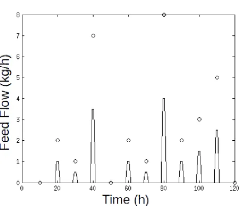
The fed-batch experiments were performed with similar conditions to those of batch experiments, 4.80 pH and 50 mM citrate buffer and 50ºC. However, the substrate an enzymatic complex were not added in the begging of the process, but, however, fed to the reactor following a feeding profile, presented in Table 4. The experiments lasted for 6h. The substrate feeding was carried out with a solids concentration of 40% in the inlet flow. The reactor initial volume was 3 L and was filled until 3.5 L.

minutes before and 2 minutes after each feeding instant.

Table 4 – Fed-Batch Feeding Profile

Time (h) Solids Feeding (g) Accumulated Solids (g)

Enzyme Feeding (g)

Accumulated Enzyme (g)

0.00 191.02 191.02 0.31 0.31

0.50 0.51 191.54 0.23 0.54

1.00 5.50 197.04 0.56 1.10

1.50 1.30 198.34 0.33 1.43

2.00 10.83 209.17 0.38 1.81

2.50 8.09 217.26 0.32 2.13

3.00 6.93 224.19 0.14 2.28

3.50 49.25 273.45 0.11 2.38

4.00 10.74 284.19 0.43 2.82

4.50 6.35 290.54 0.22 3.03

5.00 13.37 303.91 0.08 3.11

5.50 0.35 304.25 0.00 3.11

3.2. MONITORING AND CONTROL SYSTEM

This work proposes the dimensioning and construction of a system capable of monitoring, translating the data from a sensor array into a product concentration prediction, evaluating the reaction state and optimizing further activations to maximize the process efficiency. A schematic of how the system works is presented in Figure 2.

Figure 2 - Monitoring and control system

(Source: author’s collection)

3.3. EXPERIMENTAL APPARATUS

The reactor where the hydrolysis happens possesses an instrumentation array with the purpose of monitoring the free glucose concentration inside the reactive media at any given time during the hydrolysis process. The sensors measurements are relayed to a server that decodes the information, converts to the root unit of measurement when necessary and stores the data.

Figure 3 - Sensor array coupling

(Source: author’s collection) 3.3.1. Torque Measurement

The torque measurement is achieved using digital dynamometer coupled to the stirring shaft. The electric motor is above a ball bearing mount, thus the engine is free to roll in its own axle. By coupling a dynamometer perpendicularly to a rod fixated in the ball bearing a force is measured. This force is proportional to the amount of energy necessary to agitate the reactive media. To convert the straight force into stirring power, Equation 9 was used.

P=T⋅ω

_{Equation 9}

variables in Equation 10.

T

=

F⋅

L

Equation 10

Where F is the force provided by the dynamometer and L the distance of the dynamometer coupling to the center of the agitation axle. Further modifications are provided by Equation 11.

ω=

2

⋅π⋅

_N

_{Equation 11}

Where N is the rotation frequency, results in a simplification to convert the force measured by the dynamometer into stirring power presented in Equation 12.

P=

2

⋅π⋅F⋅

_L

⋅

_N

_{Equation 12}

This instrument relays data through a serial connection to a server under a RS-232 protocol. The server receives this information through a universal serial bus (USB) port and handles the data in a software layer inside a Python console. This measurement was made at every minute of the batch.

3.3.2. Supernatant Sampling and Scan

The supernatant optical properties was measured by an analytical line once an hour. The supernatant sampling begins with the filtration of the reactive media by a pumice stone filter. The driving force for the filtration was provided by a peristaltic pump. Part of the filtrated supernatant, 0.2 mL, was destined to a dilution vessel. The dilution was accomplished by a series of valves and a peristaltic pump. The dilution line worked iteratively, adding 4.0 mL per iteration, and the sample dilution necessity was assessed by the last scan, updating itself automatically.

After the dilution, the prepared sample was injected into a flow cuvette inside the spectrophotometer. With the sample properly contained, 20 scans ranging from 190 to 1100 nm was performed. This range comprehends the ultra violet and visible region of the electromagnetic spectrum. The data generated by the scans were transmitted to the server by a serial connection, under a RS-232 protocol, and the server received the information through a USB port and decoded by a software layer ran in a Python console.

The automation of sampling system was accomplished by a physical computational device for data acquisition called Arduino. The Arduino board is an open hardware platform capable of generating electronic outputs or reading inputs in a standalone method or as a slave for a server (BANZI, 2009). The signals to change the controller states are generated by a software layer coded and run in a Python console.

3.3.3. Conductivity and Capacitance Measurement

The conductivity and capacitance measurements was performed by a single probe connected to a preamplifier and transmission module Fogale Nanobiotech. The frequency used was 382 kHz.

3.3.4. Enzymatic Hydrolysis Monitoring Through Conductivity

Small-scale studies were carried out to assess how the conductivity changes inside the hydrolysis media and evaluate this methodology as a tool to monitor hydrolysis inside the reactor before adding this instrumentation a larger reactor. Three small-scale batch experiments were conducted in a 500 mL reactor, with conditions similar to the large-scale experiments. Citrate buffer at 4.80 pH and 50 mM, 10% w.v ¹ dry bagasse, 50 ºC and⁻ adding 0.17 g of enzymatic complex. In these experiments, the probe relayed its data through a serial RS-232 connection and the decoding was achieved by the proprietary software.

In the larger scales, the rest of the instrumentation was applied, however when using the capacitance/conductivity system inside the 3L reactor the acquired data by this probe was relayed to the server through a 4 to 20 mA connection. The signal was read by the data acquisition module Arduino Mega through two analog input ports, and then the data was relayed to the server via serial RS-232 connection.

3.4. CARBOHYDRATES DETERMINATION

Glucose determination was carried out manually at the offline sampling periods described in the Item 3.1. The analysis itself was performed via glucose oxidase/peroxidase enzymatic determination kit (Doles; Goiânia, GO, Brazil) and High-Performance Liquid Chromatography (HPLC).

HPLC was used to determinate glucose, xylose and cellobiose concentrations. The samples were analyzed in Shimadzu SCL-10A chromatograph using refraction index detector RID10-A, Animex HPX-87H Bio-rad, using as mobile phase sulfuric acid 5 mM at a flow of 0.6 mL.min ¹. The samples were compared to previously established standards⁻ (NREL, 2008).

Enzymatic kit analysis was used to check HPLC glucose concentration. The analysis occurred by combining 10 μmL of the prepared sample and 1 mL of the enzymatic analysis complex, incubating the mixture at 37ºC for 5 min and measuring the absorbance at 510 nm. The measured absorbance was compared to a standard curve of glucose determined with the kit in the same manner that the sample is analyzed. All analyses were performed in triplicates.

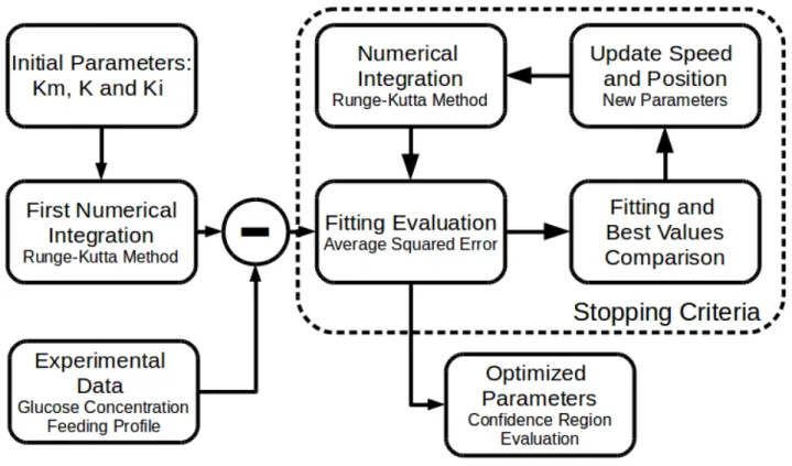
3.5. MODEL FITTING

The glucose concentrations, generated by both the batch and fed-batch experiments, were used to estimate the coefficients for the 4 models presented in item 2.4.1. In order to calculate the error between model and experimental data, simulated glucose concentration were obtained by integrating th following components balance.

dS

dt

=

F

_Substrate

V

−v

−

[

S

]⋅

F

_Substrate

V

Equation 13

dP

dt

=

v−

[

P]⋅

F

_Substrate

V

Equation 14

dE

dt

=

F

_Enzyme

V

−

[

E

]⋅

F

_Enzyme

V

Equation 15

dSol

dt

=

F

_Substrate

V

−

v

1.10

−

Xyl

⋅

v

−Cell

⋅

v

−

[

Sol

]⋅F

_Substrate

V

Equation 16

dV

dt

=F

Substrate

+

F

Enzyme Equation 17

Where [S] is the substrate concentration, FSubstrate is the inlet flow of substrate, v is

the enzymatic velocity, [P] is the product concentration, [E] is the enzyme concentration,

FEnzyme is the inlet flow of enzyme, [Sol] is the non-reactive solids concentration, Xyl and

Cell are stoichiometric empirical rates for xylose and cellobiose.

chromatographic analysis. The xylose and cellobiose concentrations are estimated from a linear fitting of these compounds and the glucose concentration. This procedure is carried separately for the batch and fed-batch experiments.

To avoid inconsistencies in the numerical solving of the model, the feeding profile cannot be a discrete vector with punctual in certain time instants. Therefore, the vector was interpolated to a continuous function throughout the time domain. A representation of this interpolation is presented in Figure 4.

Figure 4 - Interpolation Example

(Source: author’s collection) (Where: Discrete feedings (kg) at certain time instants were approximated to a continuous flow (kg.h ¹))⁻

In the Fig. 4, the blue circles represent the discrete values (optimized feeding vectors) and the blue solid line represents the generated continuous function. The interpolation algorithm behaved equally for the bagasse and enzymatic complex input profiles.

The numerical method used to integrate the differential system was a Runge-Kutta 4th _{order with variable step. Particle Swarm Optimization (PSO) algorithm was used to fit}

the parameters.

Table 5 - Particle Swarm Optimization Pseudocode # Initialization

Set Initial Parameters: Population Size, Number of Iterations, Initial Momentum, Velocity Actualization Parameters

Generates the population with random positions and velocities Generates best global and particular values and positions

Imports the experimental data for the error minimization and validation # Main Loop

While: the Number of Iterations < Maximum Iterations OR Error < Tolerance: # Error Minimization – Network Optimization

For -Each Individual in the Population:

Checks the fitting for the particle this instant

If - The present fitting is smaller than the personal bestThen:

This vector becomes the personal best (pbest) position and value End If

If - The present fitting is smaller than the swarm's best Then: This vector becomes the global best (gbest) position and value End If

# Convergence Improvement

Updates the velocity according to the best values and social parameters Decreases the swarm's momentum by a fixed value

End For

If - The number of iterations is enough Then:

Randomizes positions and velocities to reinitialized the swarm End If

End For

# Final Procedures

Tests the experimental data against the system output

During this study, the algorithms worked with a population of 10 particles and for 200 iterations. The social parameters (KENEDY & EBERHART, 2001) c1 and c2

v

_k+1

=v

_k

+c

1

∗rand

()∗(

Best

_Personal

−

x

_k

)

+

c

2

∗rand

()∗(

Best

_Global

−

x

_k

)

Equation 18 Where, vk is the particle's position, vk+1 is the next position, rand( ) is a random

number between 0 and 1, BestPersonal is the particle's position with the best fitting, BestGlobal

is the position that obtained the best fitting among all particle's and xk is the particle's

current position. The position update is presented in Equation 12.

x

_k+1

=x

_k

+

M⋅

v

_k Equation 19

Where, xk+1 is the particle's next position and M the particle's momentum.

The momentum parameter was initially set to 0.99. However, after all the particle's velocities were updated, this parameter was decreased until it reached a value lower than 0.20, after this point the momentum was reinitialized to 0.99, and positions randomization were performed. This approach is necessary to relocate the swarm from a possible local minimal point.

After the optimization procedure ends, the confidence interval for each adjusted model is calculated. An approximate confidence region can be calculated using Equation 20 (HIMMELBLAU, 1970).

C

.

_R

.

=s

_^

Yi

2

⋅F

1_−α

[

m , n−

m

]

Equation 20

Where C.R. is the confidence region range,

s

_Y^_i

2

is the standard error for each parameter, F1-α is the upper limit of the F-distribution, m is the number of parameters and n is the number of experimental data points.

The contour for the sum of squares surface can be calculated according to Equation 21.

φ=φ

_min

{

1

+

m

(n−

m)

⋅F

1_−α

[

m , n−m

]}

Equation 21

Where ϕ is the squared error threshold for the region, if a parameters group has a squared error value higher than this value it is considered outside the confidence error and

Figure 5 - Model Fitting Flowchart

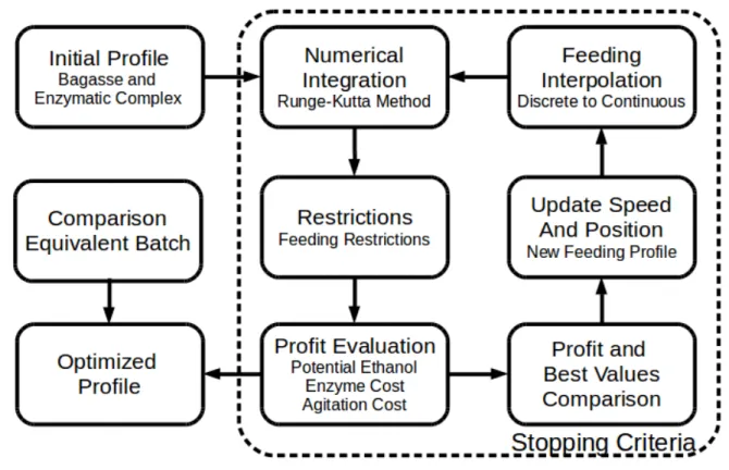
(Source: author’s collection) 3.6. FED-BATCH OPTIMIZATION

With the optimized models and its optimized parameters, the balance presented in item 3.5 was used to optimize the feeding strategy. The mass flow were subjected to an optimization method, where the profiles, both for substrate and enzymatic complex, changed at each iteration until an optimum bagasse and enzymatic complex addition is achieved.

The sequential approach and PSO algorithm, described in the previous item, were used to solve the optimal control problem. Therefore, the input flow had to be parameterized. Vectors with equal amount of points for bagasse and enzyme addition were created. The first value is the initial compound addition, and the other points are additions throughout the process.

of the enzymatic complex and electrical power necessary to agitate the reactor. This value is divided by the total mass of bagasse added in the process in order to generate a revenue related to the added mass (US$.kgBagasse⁻¹). Hence the objective function

becomes:

P

(

US $

kg

_bagasse

)=

m

_Ethanol

⋅P

_Ethanol

−m

_Enzyme

⋅

P

_Enzyme

−

P

_Power

∫

t0

tf

P

_Agitation

m

_Bagasse

Equation 22 Where P is the Performance Index (PI) generated by the process, mEthanol is the

glucose concentration converted to potential Ethanol, Pethanol is the Ethanol selling price,

mEnzime is the accumulated enzyme mass, Penzyme is the Enzymatic Complex price, Ppower is

the electric energy price, and PStirring is the power necessary to agitate the reactor.

The price for ethanol was 1.50 US$.kg ¹ (FURLAN et al. 2012), the evaluated cost⁻ of the accumulated enzymatic complex mass was 1.20 US$.kg ¹ (FURLAN et al., 2012)⁻ and the electrical power cost was 59.00 US$.Mwh ¹ (DIAS 2011). The solids fraction in the⁻ feeding flow was 0.40. The total times of fed-batch utilized in the optimization were; 360, 240, 144, 120, 96 and 48 h and feeding points were realized once an hour. The simulated reactor initial volume was 10 m³ and throughout the simulations no final reactor volume was applied.

A representation of how the optimization works is presented in Figure 6.

During the optimization, a series of restriction may be applied, to generate more feasible solutions. The profiles were subjected to maximum mass addition and maximum substrate concentrations at any given time.

Figure 6 - Feeding profile optimization

(Source: author’s collection) 3.6.1. Stirring Power

A vital part of the process PI is the cost of energy in order to agitate the reactor. To estimate this cost a relation between the solids inside the reactor and the engine torque, and subsequent stirring power.

In order to achieve this relation, an empirical model was fitted between the stirring power acquired by monitoring system and the solids inside the reactor. However, solids concentration is not available experimentally. Thus, after the most accurate enzymatic velocity model is chosen, the model is adjusted to each batch experiment following the methodology presented in item 3.5. The balance of the solids output was used in the fitting of the empirical solids/stirring power model.

3.6.2. Hydrolysis Reactor Plant Equivalence

At the end of each optimization cycle, when the optimum profile was achieved, an extrapolation was performed to determine the reactor size necessary to operate a second generation ethanol production plant.

sugarcane. This generates, approximately, 132 t.h ¹ of bagasse, 20% of this bagasse was⁻ assumed to be used to produce second generation ethanol. Thus, the 2G plant must be able to process 26.4 tbagasse.h ¹. To estimate the necessary reactor volume, or the volume⁻

sum of parallel reactors, the total processed bagasse was divided by the reactor final volume and process total time. This calculation is shown in Equation 23.

H

.

_C

.

(

t

bagasse

h

⋅

m

³

)=

m

_{Accumulated Bagasse}

t

_f

⋅

V

_f Equation 23

Where H.C. is the hydrolysis capacity of the process, mAccumulated Bagasse is the total accumulated bagasse throughout the process, tf is the process total time and Vf is the

process volume at the final time.

This value was then multiplied by the necessary productivity (26.4 tbagasse.h ¹)⁻

resulting in the volume necessary to process at this rate. 3.7. NEURAL NETWORK OPTIMIZATION

Neural Network (NN) models were used to translate the data from dynamometer and conductivity/capacitive probe to glucose concentration. The NN models were implemented in software Matlab 2012 using the Neural Network Toolbox.

The NN inputs were originated in the data provided by the instrumentation and the reactor state during the high volume batch and fed-batch hydrolysis and were: stirring power per reactor litter, conductivity, capacitance, accumulated substrate feeding and reactor volume; and the network output was the glucose concentration from the chromatography analysis. However, there were too few glucose experimental data points to train the NN correctly. To improve the network inference, the best kinetic model was adjusted for each experiment and the model predicted values were used in the network optimization.

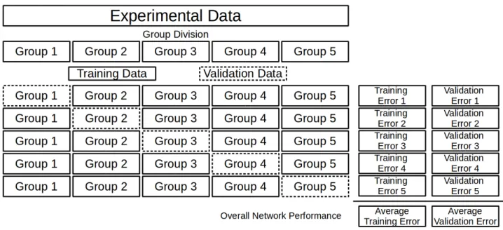
presented in Figure 7.

Figure 7 – Cross Validation Procedure

(Source: author’s collection)

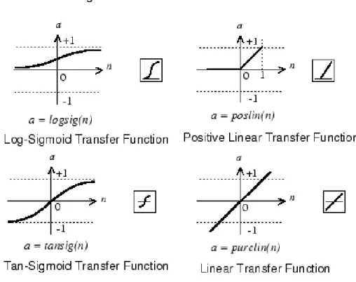
The architectures taken into account were multilayer perceptrons with one hidden layer, the numbers of neurons in the hidden layer were 1, through 15. And the evaluated transfer functions for the hidden layer and the sum layer are displayed in Figure 8. Each transfer function was evaluated both for the hidden layer and the sum layer.

The NN optimum architecture is achieved when the average standard error from the validation departs from the linear tendency of accompanying the average standard error from the training. When this happens, a possible interpretation is that the complexity of the networks has become larger than the necessary for the system. The networks starts to contemplate, in the pattern recognition, the noise from the samples disrupting the network inference (overfitting).

Figure 8 - Evaluated transfer functions

(Source: author’s collection, adapted from Matlab Neural Network Toolbox User's Guide) Figure 9 - Training and Validation Data set Error

4. RESULTS AND DISCUSSION

4.1. CONDUCTIVITY MONITORING

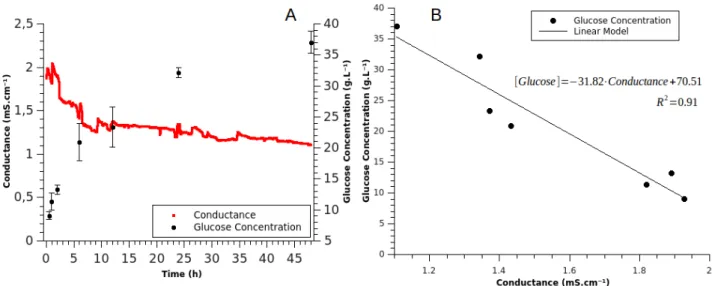
The experiments conducted in the 500 mL vessel provided the data presented in Figure 10.

Figure 10 - Conductance and glucose concentration during hydrolysis.

(Source: author’s collection) (Where: Error bars are s.d. of triplicate measurements.)

A linear negative correlation between conductance and glucose concentration in the medium supernatant was observed (see Figure 10 B), slope of -31.82, intercepting point of 70.51 and determination coefficient of 0.91. Thus, conductance may be a feasible option to follow real-time hydrolysis kinetics within the reactor. This motivates further studies using CCS to monitor the process.

Thus the conductance/capacitance probe was installed in the 3 L reactor to continue the studies.

4.2. FULL ARRAY INSTRUMENTATION

Figure 11 - Full Array Monitoring During Batch Experiments

(Source: author’s collection)

Figure 12 - Full Array Monitoring During Fed-batch Experiments

(Source: author’s collection)

The capacitance/conductance probe and dynamometer were able to monitor the experiments throughout the process. However, the analytical line and supernatant UV/VIS scanning did not show a level of robustness necessary for the application.

generated a cake on the filter membrane, which introduced a pressure drop that the used pump was not able to overcome, disabling the analytical line. Nevertheless, examples of sample scans in time periods where the analytical line was operating are presented in Figure 13, for the fed-batch experiments.

Figure 13 – Supernatant Scans During Fed-batch Experiments

(Source: author’s collection)

The data curves overlapping hinders a better analysis, thus Figure 14 presents an amplification of the range between 220 and 400 nm.

Figure 14 – Supernatant Scans from 250 to 320 nm

(Source: author’s collection)