ABSTRACT: The present study faces the problem of safely controlling the position trajectory of a multirotor aerial vehicle subjected to a conic constraint on the total thrust vector and a linear convex constraint on the position vector. The problem is solved using a linear state-space model predictive control strategy, whose optimization is made handy by replacing the original conic constraint set on the thrust vector by an inscribed pyramidal space, which renders a linear set of inequalities. The proposed method is evaluated on the basis of Monte Carlo simulations taking into account a random disturbance force. The simulation results show the effectiveness of the method in tracking the commanded trajectory while respecting the constraints. They also predict the effect of both the speed command and the maximum allowed inclination angle on the system performance.
KEYWORDS: Multirotor aerial vehicle, Model predictive control, Position control, Guidance.
A Model Predictive Guidance Strategy for
a Multirotor Aerial Vehicle
Igor Afonso Acampora Prado
1, Davi Antônio dos Santos
1INTRODUCTION
Unmanned Aerial Vehicles (UAVs) have motivated and stimulated many researches in diferent ields of knowledge such as sensors fusion (Cheviron et al. 2007; Nemra and Aouf 2010; Gonçalves et al. 2013), computer vision (Saripalli et al. 2003; Xu et al. 2009; Xiao-Hong et al. 2012) and control strategies (Mian and Daobo 2008; Santos et al. 2013). A few years ago, building a low-cost miniature UAV was a challenge due to limitation imposed by equipment such as sensors, eicient motors, batteries and on-board computers. However, thanks to technological advances in actuators, small scale sensors, data processing and energy storage, the conditions improved signiicantly.
Among the diferent types of UAVs such as blimps (Elfes
et al. 1998), ixed-wings (Beard et al. 2005) and rotary wings aircrats (Bouabdallah et al. 2004), the present study focuses on the multirotor aerial vehicles (MAVs) (Gupte et al. 2012; Er et al. 2013). he interest for MAVs has increased in the last decade due to their low cost, high maneuverability, simpliied mechanics, capability to perform vertical take-of and landing as well as hovering light. hese characteristics make them suitable for a wide range of applications, such as surveillance of indoor and urban environments, object delivery, building inspection, and agriculture monitoring. In all the aforementioned applications, a precise position tracking controller (or a guidance law) is crucial for autonomous operation.
Although there is a massive amount of concluded and ongoing research studies on MAVs, the design of control laws for such vehicles still has challenges to overcome. Most of those challenges are related to safety of the MAV itself and for people close to its operation. Mistler et al. (2013) and
Mahony et al. (2012) propose linear control laws combined with the feedback linearization technique for guiding a quadrotor through a reference trajectory. Bouabdallah and Siegwart (2005) designed 2 control laws using, respectively, the sliding mode and the backstepping methods; the authors showed by simulations that the backstepping method outperforms the sliding mode controller. Madani and Benallegue (2007) propose position control scheme combining a backstepping controller with a sliding mode observer. Castillo et al. (2014) and Hua et al. (2009) present robust control law design methods considering that the system is subjected to external disturbance and model uncertainty. It is worth mentioning that none of the aforementioned methods have considered constraints on the control force.
In fact, few MAV control methods available in the literature have dealt with constraints issues (Castillo et al. 2005; Cunha
et al. 2009). In Castillo et al. (2005), the authors divided the system into smaller subsystems with 2 degrees of freedom (DOF). For each subsystem, they applied a nested saturated controller (Teel 1992) to achieve global stability while respecting a maximum constraint on the total thrust magnitude. However, the subsystems were assumed to have uncoupled dynamics, which is not true in general. In Cunha et al. (2009), to avoid an unbounded growth of the actuation commands, the authors presented an asymptotically stable controller that limits the maximum thrust magnitude by saturating the position control error. These 2 studies only considered constraints on the maximum value of the magnitude of the total thrust vector.
More recently, Santos et al. (2013) and Yan et al. (2014) tackled the problem of controlling the position of an MAV under constraints both on the inclination of the rotor plane and on the magnitude of the total thrust. Santos et al. (2013) presented a simple but efective control method derived using feedback linearization and a proportional-derivative control law. Yan et al. (2014) solved the same problem by using the retrospective cost adaptive control (RCAC) strategy.
he model predictive control (MPC) strategy appears as the most interesting choice whenever constraints are a concern. In this method, a future control sequence is obtained by minimizing a cost function on predicted values of the controlled variable along a inite horizon, typically subjected to constraints (Camacho and Bordons 1998). Applications of MPC to position control of MAVs can be found in Rafo et al. (2010), Lopes et al. (2011), Alexis et al. (2012), and Chen
et al. (2013). Rafo et al. (2010) proposed a control scheme
consisting of an unconstrained MPC for position tracking and a non-linear H∞ controller for attitude stabilization under aerodynamic disturbances and parametric as well as structural uncertainties. Lopes et al. (2011) designed a single MPC controller for both position control and attitude stabilization, considering constraints on both the pitch and the roll angles. Alexis et al. (2012) proposed a cascade MPC scheme, formulated over a set of piecewise aine models originated from both attitude and translation dynamics. In order to guide an MAV through a desired position trajectory, Chen et al. (2013) designed 2 separate MPCs, one for position control and the other for attitude control, the latter considering maximum constraints on the attitude angles.
In order to ensure a safe light, it is essential to design a control law which avoids excessive accelerations and unexpected lips. he present study proposes an MPC for position control (guidance) of an MAV, constraining the total thrust vector within a conic set as well as the position vector within a parallelepiped set.
PROBLEM STATEMENT
PRELIMINARY DEFINITIONS
he motion of an MAV has 6 DOFs: 3 in translation and other 3 in rotation. However, this vehicle has only 4 independent control inputs: 3 torque components and the magnitude of the total thrust. Therefore, an MAV has an underactuated dynamics. At a irst glance, it could be seem a challenge to deal with this characteristic. However, in practice, one needs to independently control only 4 DOF: the 3-dimensional position and the heading angle.
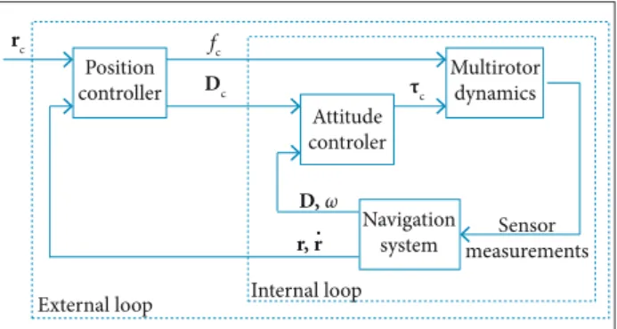
he block diagram of Fig. 1 describes a control system for controlling the 3-dimensional position r∈ℝ3 of an MAV to follow a time-varying position command r
c∈ℝ
3. This
Figure 1. A typical structure of an MAV light control system.
Position controller
Sensor measurements
rc fc
Internal loop
Navigation system
Dc
r, r. D , ω
τc
Attitude controler
Multirotor dynamics
system is structured into 2 control loops: an internal loop for attitude control and an external one for position control. h e Navigation System is generally responsible for estimating the vehicle’s attitude D∈ SO(3), angular velocity ω ∈ℝ3, position
r, and linear velocity r . ∈ℝ3 . h e Attitude Controller receives an attitude command Dc∈ SO(3) and produces the control torque τc∈ℝ3 necessary to rotate the rotor plane with respect to the local horizontal plane. h e Position Controller has the function of computing a command fc∈ℝ3 for the total thrust magnitude and a command Dc∈ SO(3) for the attitude. h ese commands are computed in such a way to produce suitable lateral acceleration on the vehicle. h e present study is concerned with the design of a position controller.
POSITION CONTROL PROBLEM
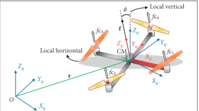
Consider the MAV and the 3 Cartesian coordinate systems (CCS) illustrated in Fig. 2. Assume that the vehicle has a rigid structure. h e body CCS SB= ∆ {XB, YB, ZB} is i xed to the structure and its origin coincides with the vehicle’s center of mass (CM). h e reference CCS SR= ∆ {XR, YR, ZR} is Earth-i xed and its origin is at a known point O. Finally, a second reference CCS SR'= ∆ {XR', YR', ZR'} is dei ned to be parallel to SR, but with origin at CM. Assume that SR is an inertial frame.
with respect to SR; f= ∆ [fx, fy, fz]T∈ℝ3 is the total thrust vec-tor represented in SR; fd∈ℝ3 is the disturbance force vector represented in SR, m is the vehicle’s mass; g is the gravitational acceleration.
If, instead of a quadrotor, we had considered a hexa-rotor or an octo-hexa-rotor, the model in Eq. 1 would not change in any aspects, except for the origin of f that would receive contributions of either 6 or 8, instead of 4 propellers. As illustrated in Fig. 2, f is perpendicular to the rotor plane.
Dei ne the inclination angle ϕ∈ℝof the rotor plane as the angle between ZB and ZR’. It can be expressed by
Figure 2. A multirotor aerial vehicle and 3 Cartesian coordinate systems.
ZR
YR
ZR’
ZB YB
XB YR’
XR’
XR
O
r
f ϕ
Local horizontal CM
Local vertical
fc3
fc2
fc1 fc4
Invoking the second Newton’s law, the translational dynamics of the MAV illustrated in Fig. 2 can be immediately described in SR by the following second-order dif erential equation:
where: r= ∆ [rx, ry, rz]T∈ℝ3 is the CM position vector
(1)
(2)
(3)
where: fc= ∆ ||f||.
Dei ne the position control error r ~∈ℝ3 as
where: rc= ∆ [rc,x rc,y rc,z]T is a position command. Problem 1: ϕ
max∈ℝ denote the maximum allowable value of ϕ, fmin∈ℝ and fmax∈ℝ denote, respectively, the minimum and maximum allowable values of fc, and rmin ∈ℝ3 and rmax∈ℝ3 denote, respectively, the minimum and maximum allowable values of r. h e MAV guidance problem is to i nd a control law for f that minimizes r ~ subjected to the inclination constraint
ϕ ≤ ϕmax, to the force magnitude constraint fmin ≤ fc≤ fmax, and to the position constraint rmin ≤ r ≤ rmax.
Remark 1: the control force f of Problem 1 is not the ef ective
control force undergone by the vehicle. In fact, its magnitude
fcrepresents a command for the power electronics to drive the motors, while the inclination angle ϕ is used to compute the attitude command Dc for the attitude control loop to orient the rotor plane (Fig. 1). Nevertheless, fc and Dc are assumed here to be identical to the respective actual variables. h e assumption about fc is reasonable if a precise model for the thrust force is available. On the other hand, the assumption about Dc can also be approximated in practice if the controllers are tuned to allow the internal loop to have a much faster dynamics than the external one.
Remark 2: during the design of the controller, disturbance
Remark 3: the position r and the velocity . r of CM are
assumed to be available for feedback. In practice, these variables are provided by a navigation system (Fig. 1), which is not the focus of the present study.
In Problem 1, the parallelepiped constraint imposed on the vehicle’s position r is considered so as to avoid collisions with the bounds of a box-shaped indoor environment.
On the other hand, one can visualize the corresponding constraint space on f as a conic space with an inferior and a superior spherical lid, as illustrated in Fig. 3. Note that the so-generated constraint space is non-linear and non-convex. h e constraints on both magnitude and inclination of f are directly connected to the vertical and lateral accelerations of the vehicle. As one can see in Fig. 4, the component fzis responsible for controlling the altitude of the vehicle, while fxy
produces the lateral acceleration that guides it along the XR and
YR directions, where fxy= ∆ [fx fy] ∈ℝ2 denotes the horizontal projection of f. As ϕ increases, the lateral acceleration of the vehicle also increases. If the constraint fmax is not sui ciently high, the vehicle could suf er a loss of lit . Furthermore, it is interesting to choose a ϕmax that avoids unexpected l ips as well as large lateral accelerations.
h e choice of suitable values for the constraints on f and r
can enhance the l ight safety, since it avoids abrupt motion and delimits the l ight region, respectively. Such characteristics are quite desirable, for example, in MAVs used to support people in indoor and urban environments.
PROBLEM SOLUTION
STATE-SPACE MODEL FOR TRANSLATION
Dei ne the state vector x= ∆ [rx r .x ry r .y rz r .z]T∈ℝ6 and the control input vector u= ∆ [ux uy uz]T∈ℝ3,
fmax
fmin
ϕmax
ϕ
f
ZR’
ZB
Local horizontal CM
Figure 3. The original conic control space.
Figure 4. Analysis of f with respect to its constraints on inclination and magnitude.
Using Eq. 4, Eq. 1 can be immediately rewritten as a continuous-time linear state equation of the form x .= Ax + Bu. Similarly, by dei ning the controlled output vector to be the MAV position y= ∆ [rx ry rz]T∈ℝ3, one can obtain a continuous-time output equation of the form y = Cx. Let x(k) ∈ ℝ6, u(k) ∈ ℝ3 and y(k) ∈ ℝ3 denote, respectively, the state vector, the control input vector and the controlled output vector, all in the discrete-time domain. Using the ZOH method with a sampling time of Ts = 20 ms, a discrete-time version of the above state-space model is obtained as
(4)
(5)
(6)
(7)
where
Reference trajectory Local vertical
Local horizontal
fmax
Consider the discrete-time state-space model of Eqs. 5 and 6. It can be rewritten in the incremental-input form as (Maciejowski 2002)
a prediction horizon of length N; ∆uM∈ℝ3M ×1 stacks the incremental control inputs along a control horizon of length M,
(8)
(9)
(10)
(11)
(12)
(13)
(14)
(15)
(16)
(17)
(18)
(19)
(20)
with
where: ∆x(k) = ∆ x(k) –x(k –1) ∈ℝ6 denotes the incremental state vector; ∆u(k) = ∆ u(k) –u(k –1) ∈ℝ3 is the incremental control input vector; I3 is the identity matrix with dimensions 3 × 3; 03 ×6 is a zero matrix with dimensions 3 × 6.
PREDICTION MODEL
Using Eq. 10, the prediction model can be obtained as (see Maciejowski 2002, p. 50)
where: γN∈ℝ3N×1 stacks the controlled outputs along
and
THRUST VECTOR CONSTRAINTS
Using Eq. 4, the thrust magnitude constraint inequation
fmin≤ fc≤ fmax can be rewritten in terms of u as
Assuming that 0 ≤ ϕmax< π/2 rad, the inclination cons-traint ϕ ≤ ϕmax established in Problem 1 can be replaced by cos ϕ ≥ cos ϕmax . Using Eqs. 2 and 4, the last inequation can be rewritten in terms of the components of u as
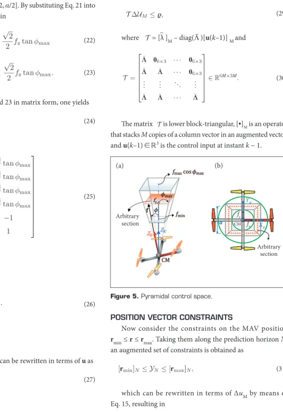
In order to obtain linear approximations for Eqs. 18 and 19, consider the rectangular pyramid inscribed in the original conic control space depicted in Fig. 3. h e new control space is illustrated in Fig. 5a. By inspection of this i gure, the new constraint on fz can be expressed as
α × α, as illustrated in Fig. 5b. From the geometry of this i gure, one can write
Finally, replacing u(k) = Δu(k) + u(k–1) into Eq. 27 and taking it at M future instants starting from k, the thrust vector constraint is obtained as
(21)
(22)
(23)
(24)
(25)
(26)
(27)
By inspection of Fig. 5b, it can be seen that the implication of f to be bounded inside the pyramidal space is that
fx∈ [–α/2, α/2] and fy∈ [–α/2, α/2]. By substituting Eq. 21 into these intervals, one can obtain
Rewriting Eqs. 20, 22 and 23 in matrix form, one yields
where
Figure 5. Pyramidal control space.
arbitrary section
fx fy
α CM
Arbitrary section arbitrary
section
fx fx fx fx fy fy fy
fy
YR’
α
XR’
Arbitrary section
fx
max
and
Now using Eq. 4, Eq. 24 can be rewritten in terms of u as
where Λ –= ∆mΛ and
(28)
(29)
(30)
(31)
where = [λ –]M – diag(Λ –)[u(k–1)] Mand
h e matrix is lower block-triangular, [•]M is an operator that stacks M copies of a column vector in an augmented vector, and u(k–1) ∈ℝ3 is the control input at instant k − 1.
POSITION VECTOR CONSTRAINTS
Now consider the constraints on the MAV position
rmin ≤ r ≤ rmax. Taking them along the prediction horizon N, an augmented set of constraints is obtained as
which can be rewritten in terms of ΔuM by means of Eq. 15, resulting in
(a) (b)
w h ere
input u(k) provided by the MPC. h e i rst command is obtained by simply taking the Euclidian norm of f. Using Eq. 4, fc is obtained as
(32)
(33)
(34)
(35)
(36)
(37)
(38)
and
MODEL PREDICTIVE CONTROLLER
The optimal control vector u*(k) ∈ℝ3 computed at the discrete-time instant k is given by u*(k) = Δu*(k) + u*(k–1), where Δu*(k) ∈ℝ3 is the i rst control vector in Δu*M, which, in turn, is obtained by minimizing the following quadratic cost function:
subjected to
where: 1/2H = GTQG + R, MT = 2(F – [r c]N)
TQG,
c = (F – [rc]N)TQ (F – [r c]N),
and
In this study, the controlled output weighting matrix is set to Q = η × I3N and the control input weighting matrix is set to
R = ρ × I3M. h e above optimization problem is in the conventional quadratic programming form, for which there are efficient numerical solution methods (Rossiter 2003). The Δ-input MPC formulation presented here has an intrinsic integral action, which allows to track a constant set point with 0 steady-state error and reject a constant disturbance input (Maciejowski 2002).
THRUST MAGNITUDE AND ATTITUDE COMMANDS
Now we need to compute the total thrust magnitude command fc and the attitude command Dc from the control
(39)
(40)
(41)
(42)
(43)
h e attitude command Dc∈ SO(3) for the internal (attitude) control loop (Fig. 1) is also computed from f, which contains information about the orientation of the rotor plane with respect to the local horizontal. In order to provide a unique 3-dimensional attitude command, it is necessary to specify a heading angle. For example, one can choose a 0 heading angle, which is just equivalent to the attitude represented by the principal Euler angle/axis (ϕ; e), where ϕ is computed from Eq. 2 and e is a unit vector given by
where: fxy is the projection of f on the XR’– YR’ plane. h e corresponding attitude command is given by (Shuster 1993)
Now considering an arbitrary heading angle ψ, the attitude command Dcresults from 2 successive rotations. The first one is that represented by Eq. 41, while the second one is an elementary rotation D(ψ; ZB)of an angle ψ about the ZBaxis, i.e.
where
COMPUTATIONAL SIMULATIONS
SIMULATION PARAMETERS
h e interior-point method is adopted to solve the MPC optimization. The control input weighting matrix Q and controlled output weighting matrix R are adjusted with ρ = 0.01 and η = 1, respectively. h e prediction and control horizons are set to N = 80 and M = 5, respectively. h e maximum and minimum position bounds are rmax = [6 6 3]Tm and r
min = [0 0 0] T,
respectively. h e maximum and minimum constraints on the force magnitude are set in fmax = 20 N and fmin = 2 N, respectively. A non-zero minimum bound on the force magnitude fminwas chosen in order to avoid loss of attitude control. On the other hand, the maximum bound fmax is set sufficiently large to allow lateral accelerations without loss of lit . In order to verify the system robustness against an unknown input, a 0-mean Gaussian disturbance force with covariance Qd = 0.3× I3 N2 is taken into account.
The position commands consist of a sequence of line segments from the initial position ri= [1 1 0]T m to the i nal one rf= [5 5 1]T m passing by the waypoints w
1 = [1 1 1]
T m;
w2 = [2 2 2]T m; w
3 = [4 2 2]
Tm; w
4 = [5 3 2]
T m and
w5 = [5 5 2]T m. A total of 15 MC simulations with 300
realizations are carried out considering all the combinations of 3 dif erent speed command v values (0.5; 1.0 and 2.0 m/s) and 5 dif erent maximum inclination ϕmax values (10°; 15°; 20°; 25° and 30°).
h e following i gure of merit is used to evaluate the position control error:
(44)
(45)
h e attitude controllers chosen for the present simulation are uncoupled proportional-derivative control laws tuned so as to make the attitude dynamics have a bandwidth signii cantly larger than the bandwidth of the position control dynamics.
SIMULATION RESULTS
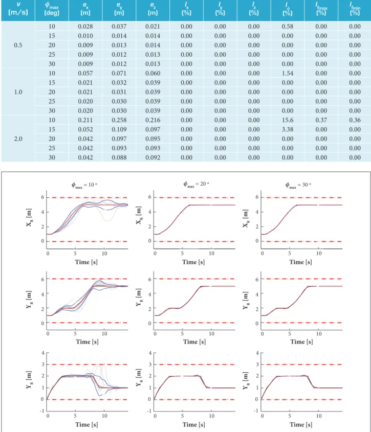
h e Monte Carlo simulation results are summarized in Table 1 in terms of eq and Il. First, one can observe that the con-trol error increases as the speed command v is increased or as the maximum inclination ϕmax is decreased. For example, for
v = 0.5 m/s, the position errors stay below 5 cm, whereas they approach 25 cm when the speed is set to v = 2.0 m/s. Regarding the violation of position constraints, no occurrence is observed with any of the 3 speed commands. Concerning the maximum inclination constraint ϕmax, for all speed commands v, the number of violations reduces as ϕmax is increased. Finally, the frequency of violations of fmin and fmaxincreases as the speed command is increased, but decreases as ϕmax is increased.
Figure 6 shows the MC realizations of the MAV position together with the corresponding mean and standard deviation curves for v = 1.0 m/s and dif erent values of ϕmax (10°; 20°; 30°). One can see that the standard deviation decreases as ϕmaxincreases. h is behavior is due to the fact that a smaller value of ϕmax results in a smaller horizontal projection fxyof the total thrust on the horizontal plane, which, in turn, reduces the vehicle’s maneuverability and capability to reject horizontal disturbance forces. On the contrary, as ϕmax increases, fxybecomes larger, improving the maneuverability, which, in turn, provides a better disturbance rejection.
On the other hand, Fig. 7 shows the MC realizations of the MAV position together with the corresponding mean and standard deviation curves for ϕmax = 15° and dif erent values of v (0.5; 1.0 and 2.0 m/s).
One can see that, as the speed command increases, the standard deviation also becomes larger. The main reason is the fact that larger speed commands require better maneuverability and larger horizontal acceleration to ensure that the vehicle follows the reference trajectory with acceptable performance. h e worst performance observed in Table 1 occurs with
ϕmax= 10° and v = 2.0 m/s. This scenario combines low maneuverability (due to a small ϕmax) with a large speed command, which results in a large amount of control input constraint violations (Fig. 8). With a small ϕmax, the vehicle does not reach sui cient lateral acceleration to follow a large speed command and simultaneously reject the disturbance force. It causes a large position error (Fig. 9).
for q equal to x, y or z; r(i)
q(k) denotes the i
th realization
of rq(k).
For evaluating the frequency of constraint violation, the following i gure of merit is adopted:
(46)
Table 1. Monte Carlo simulation results for different values of v and ϕmax. v (m/s) ϕmax (deg) e x (m) e y (m) e z (m) I x (%) I y (%) I z (%) I ϕ (%) I fmax (%) I fmin (%)
0 . 5
1 0 0 . 0 2 8 0 . 0 3 7 0 . 0 2 1 0 . 0 0 0 . 0 0 0 . 0 0 0 . 5 8 0 . 0 0 0 . 0 0 1 5 0 . 0 1 0 0 . 0 1 4 0 . 0 1 4 0 . 0 0 0 . 0 0 0 . 0 0 0 . 0 0 0 . 0 0 0 . 0 0 2 0 0 . 0 0 9 0 . 0 1 3 0 . 0 1 4 0 . 0 0 0 . 0 0 0 . 0 0 0 . 0 0 0 . 0 0 0 . 0 0 2 5 0 . 0 0 9 0 . 0 1 2 0 . 0 1 3 0 . 0 0 0 . 0 0 0 . 0 0 0 . 0 0 0 . 0 0 0 . 0 0 3 0 0 . 0 0 9 0 . 0 1 2 0 . 0 1 3 0 . 0 0 0 . 0 0 0 . 0 0 0 . 0 0 0 . 0 0 0 . 0 0
1 . 0
1 0 0 . 0 5 7 0 . 0 7 1 0 . 0 6 0 0 . 0 0 0 . 0 0 0 . 0 0 1 . 5 4 0 . 0 0 0 . 0 0 1 5 0 . 0 2 1 0 . 0 3 2 0 . 0 3 9 0 . 0 0 0 . 0 0 0 . 0 0 0 . 0 0 0 . 0 0 0 . 0 0 2 0 0 . 0 2 1 0 . 0 3 1 0 . 0 3 9 0 . 0 0 0 . 0 0 0 . 0 0 0 . 0 0 0 . 0 0 0 . 0 0 2 5 0 . 0 2 0 0 . 0 3 0 0 . 0 3 9 0 . 0 0 0 . 0 0 0 . 0 0 0 . 0 0 0 . 0 0 0 . 0 0 3 0 0 . 0 2 0 0 . 0 3 0 0 . 0 3 9 0 . 0 0 0 . 0 0 0 . 0 0 0 . 0 0 0 . 0 0 0 . 0 0
2 . 0
1 0 0 . 2 1 1 0 . 2 5 8 0 . 2 1 6 0 . 0 0 0 . 0 0 0 . 0 0 1 5 . 6 0 . 3 7 0 . 3 6 1 5 0 . 0 5 2 0 . 1 0 9 0 . 0 9 7 0 . 0 0 0 . 0 0 0 . 0 0 3 . 3 8 0 . 0 0 0 . 0 0 2 0 0 . 0 4 2 0 . 0 9 7 0 . 0 9 5 0 . 0 0 0 . 0 0 0 . 0 0 0 . 0 0 0 . 0 0 0 . 0 0 2 5 0 . 0 4 2 0 . 0 9 3 0 . 0 9 3 0 . 0 0 0 . 0 0 0 . 0 0 0 . 0 0 0 . 0 0 0 . 0 0 3 0 0 . 0 4 2 0 . 0 8 8 0 . 0 9 2 0 . 0 0 0 . 0 0 0 . 0 0 0 . 0 0 0 . 0 0 0 . 0 0
0 5 10
0 2 4 6
φmax = 10o
XR
[m
]
0 5 10
0 2 4 6 YR [m ]
0 5 10
-1 0 1 2 3 4 Time [s] ZR [m ]
0 5 10
0 2 4 6
φmax = 20o
0 5 10
0 2 4 6
0 5 10
-1 0 1 2 3 4 Time [s]
0 5 10
0 2 4 6
φmax = 30o
0 5 10
0 2 4 6
0 5 10
-1 0 1 2 3 4 Time [s] 6 4 2 0 1 0 0 5 6 4 2 0 1 0 0 5 6 4 2 0 1 0 0 5 6 4 2 0 1 0 0 5 6 4 2 0 1 0 0 5 6 4 2 0 1 0 0 5 3 4 2 0 1 -1 1 0 0 5 3 4 2 0 1 -1 1 0 0 5 3 4 2 0 1 -1 1 0 0 5
ϕmax = 30 º ϕmax = 10 º
Ti m e [ s ] T i m e [ s ] T i m e [ s ]
T i m e [ s ] T i m e [ s ] T i m e [ s ]
T i m e [ s ] T i m e [ s ] T i m e [ s ]
XR [ m ] YR [ m ] YR [ m ] XR [ m ] YR [ m ] YR [ m ] XR [ m ] YR [ m ] YR [ m ]
ϕm a x = 20 º
0 10 20 0
2 4 6
v = 0.5 m/ s
X
R[m
]
0 10 20
0 2 4 6
Y
R[m
]
0 10 20
-1 0 1 2 3 4 Time [s]
Z
R[m
]
0 5 10
0 2 4 6
v = 1 m/s
0 5 10
0 2 4 6
0 5 10
-1 0 1 2 3 4 Time [s] 0 5 0 2 4 6
v = 2 m/s
0 5 0 2 4 6 0 5 -1 0 1 2 3 4 Time [s] 6 4 2 0 20 0 10 XR [ m ] 6 4 2 0 10 0 5 6 4 2 0 0 5 6 4 2 0 0 5 6 4 2 0 20 0 10 YR [ m ] 6 4 2 0 10 0 5 3 4 2 0 1 -1 3 4 2 0 1 -1 20
0 10 -10 5 10
3 4 2 0 1 -1 5 0 ZR [ m ] XR [ m ] YR [ m ] ZR [ m ] XR [ m ] YR [ m ] ZR [ m ]
Ti me [s ] Time [s] Time [s]
Time [s] Time [s] Time [s]
Time [s] Time [s] Time [s]
v = 1 m/s
v = 0.5 m/s v = 2 m/s
Figure 7. Performance of position control varying the speed command. The solid gray lines are MC realizations; the dashed red lines are the position constraints; the solid black lines are the position command; the solid red lines are the sample means; the solid blue lines are the sample means plus/minus the standard deviation.
Figure 8. Inclination angle ϕ and thrust magnitude fc in the worst case (ϕmax = 10° and v = 2.0 m/s). The gray lines are the
MC realizations and the dashed red lines are the constraints.
In c l i n a t i o n a n g l e
Time [s] 0
0 100 200
1 2 3 4 5 6 7 8 9
ϕ
[deg]
Time [s] Total thrust magnitude
fc [N] 0 0 10 20
1 2 3 4 5 6 7 8 9
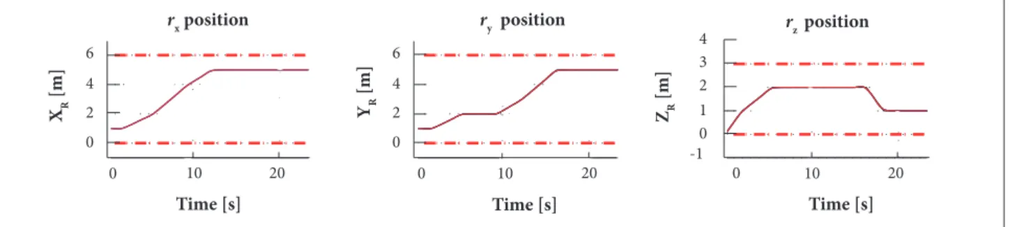
On the other hand, the best performance observed in Table 1 occurs with ϕmax = 30° and v = 0.5 m/s. his scenario combines high maneuverability (due to a large ϕmax) with a small speed command. In this case, the vehicle does not sufer a signiicant inluence of
the disturbance forces and respects the constraint on both the inclination angle ϕ and thrust magnitude fc. For details, Fig. 10 shows
Figure 9. Performance of position control in the worst case (ϕmax = 10° and v = 2.0 m/s) . The solid gray lines are MC realizations; the dashed red lines are the position constraints; the solid black line are the position commands; the solid red lines are the sample means; the solid blue lines are the sample means plus/minus the standard deviations.
Figure 11. Performance of position control in the best case (ϕmax = 30° and v = 0.5 m/s). The solid gray lines are MC realizations; the dashed red lines are the position constraints; the solid black lines are the position commands; the solid red lines are the sample means; the solid blue lines are the sample means plus/minus the standard deviations.
6
4
2
0
0 5
6
4
2
0
0 5
3 4
2
0 1
-1
5 0
Time [s] Time [s]
Time [s]
YR
[m]
XR
[m]
ZR
[m]
r
x position ry position rzposition
0 10 20
0 2 4 6
rx Position
Tim e [s]
X
R[m
]
0 10 20
0 2 4 6
ry Position
Tim e [s]
Y
R[m
]
0 10 20
-1 0 1 2 3 4
rz Position
Tim e [s]
Z
R[m
]
6
4
2
0
0 10
6
4
2
0
0 10
YR
[m]
3 4
2
0 1
-1
10 20
20
20 0
XR
[m]
ZR
[m]
Time [s] Time [s]
r
x position ry position rz p osition
Time [s]
Figure 10. Inclination angle ϕ and thrust magnitude fc in the best case (ϕmax = 30° and v = 0.5 m/s). The gray lines are the MC realizations; the dashed red lines are the constraints.
Inclination angle
Time [s] 0
0 20 30
10
20 10
5 15
ϕ
[deg]
Time [s] Total thrust magnitude
fc
[N]
0 5 10 15 20
0 10 20
CONCLUSIONS
Th is study tackled the problem of controlling the position
of a MAV subjected to constraints on the inclination of the rotor plane, on the total thrust magnitude, and on the position. The problem was solved using a conventional linear-quadratic state-space MPC formulation, which became
possible thanks to the replacement of the original conic constraint space on the total thrust vector by an inscribed pyramid.
REFERENCES
Alexis K, Nikolakopoulos G, Tzes A (2012) Model predictive quadrotor control: attitude, altitude and position experimental studies. IET Control Theory Appl 6(12):1812-1827. doi: 10.1049/iet-cta.2011.0348
Beard R, Kingston D, Quigley M, Snyder D, Christiansen R, Johnson W, McLain T, Goodrich MA (2005) Autonomous vehicle technologies for small ixed-wing UAVS. J Aero Comput Inform Comm 2(1):92-108. doi: 10.2514/1.8371
Bouabdallah S, Murrieri P, Siegwart R (2004) Design and control of an indoor micro quadrotor. Proceedings of the IEEE International Conference on Robotics and Automation; New Orleans, USA.
Bouabdallah S, Siegwart R (2005) Backstepping and sliding-mode techniques applied to an indoor micro quadrotor. Proceedings of the IEEE International Conference on Robotics and Automation; Barcelona, USA.
Camacho EF, Bordons C (1998) Model predictive control. London: Springer.
Castillo P, Lozano R, Dzul A (2005) Stabilization of a mini rotorcraft with four rotors. IEEE Contr Syst Mag 25(6):45-55. doi: 10.1109/ MCS.2005.1550152
Castillo P, Munoz LE, Santos O (2014) Robust control algorithm for a rotorcraft disturbed by crosswind. IEEE Trans Aero Electron Syst 50(1):756-763. doi: 10.1109/TAES.2013.110136
Chen X, Wang L, Xung J (2013) Cascaded model predictive control of a quadrotor UAV. Proceedings of the 3th Australian Control Conference; Fremantle, Australia.
Cheviron T, Hamel T, Mahony R, Baldwin G (2007) Robust nonlinear fusion of inertial and visual data for position, velocity and attitude estimation of UAV. Proceedings of the IEEE International Conference on Robotics and Automation; Rome, Italy.
Cunha R, Cabecinhas D, Silvestre C (2009) Nonlinear trajectory tracking control of a quadrotor vehicle. Proceedings of the 7th European Control Conference; Budapest, Hungary.
Elfes A, Bueno SS, Bergerman M, Ramos JG (1998) A semi-autonomous robotic airship for environmental monitoring missions.
Proceedings of the IEEE International Conference on Robotics and Automation; Leuven, Belgium.
Er MJ, Yuan S, Wang N (2013) Development control and navigation of octocopter. Proceedings of the 10th International Conference on Control and Automation; Hangzhou, China.
Gonçalves PFSM, Brusnicki R, Santos DA (2013) Attitude determination of multirotors using camera vector measurements. Proceedings of the 22nd International Congress of Mechanical Engineering; Ribeirão Preto, Brazil.
Gupte S, Mohandas PIT, Conrad JM (2012) A survey of quadrotor unmanned aerial vehicles. Proceedings of the IEEE SoutheastCon; Orlando, USA.
Hua MD, Hamel T, Morin P, Samson C (2009) A control approach for thrust-propelled underactuated vehicles and its application to VTOL drones. IEEE Trans Automat Contr 54(8):1837-1853. doi: 10.1109/ TAC.2009.2024569
Lopes RV, Santana PHRQA, Borges GA, Ishihara JY (2011) Model predictive control applied to tracking and attitude stabilization of a VTOL quadrotor aircraft. Proceedings of the 21st International Congress of Mechanical Engineering; Natal, Brazil.
Maciejowski JM (2002) Predictive control with constraints. Harlow; New York: Prentice-Hall.
Madani T, Benallegue A (2007) Sliding mode observer and backstepping control for a quadrotor unmanned aerial vehicles. Proceedings of the American Control Conference; New York, USA.
Mahony R, Kumar V, Corke P (2012) Multirotor aerial vehicles: modeling, estimation, and control of quadrotor. IEEE Robot Autom Mag 19(3):20-32. doi: 10.1109/MRA.2012.2206474
Mian AA, Daobo W (2008) Nonlinear light control strategy for an underactuated quadrotor aerial robot. Proceedings of the International Conference on Networking, Sensing and Control; Sanya, China.
Mistler V, Benallegue A, M’Sirdi N (2013) Exact linearization and noninteracting control of a 4 rotors helicopter via dynamic feedback. f orces, while respecting the position and control constraints.
However, if a large speed command is considered, it is necessary to relax the maximum inclination constraint in order to have sufficient lateral control force to overcome the disturbance forces.
he Δ-input MPC formulation used in this study appears as a good option for controlling the position of an MAV due to its ability of handling input and state constraints and, if suitably adjusted, it presents smooth responses to position commands. As the MPC has to solve an optimization problem at each update time, a drawback of this strategy is its high computational burden compared with traditional controllers such as the classic PID.
ACKNOWLEDGMENTS
he irst author would like to thank Fundação de Amparo à Pesquisa do Estado do Amazonas for providing his master scholarship during the project. Furthermore, we are grateful to Conselho Nacional de Desenvolvimento Cientíico e Tecnológico for supporting the project under the grant 475251/2013.
AUTHOR’S CONTRIBUTION
Proceedings of the 10th IEEE International Workshop on Robot and Human Interactive Communication; Bordeaux, France.
Nemra A, Aouf N (2010) Robust INS/GPS sensor fusion for UAV localization using SDRE nonlinear iltering. IEEE Sensor J 10(4):789-798. doi: 10.1109/JSEN.2009.2034730
Raffo GV, Ortega MG, Rubio FR (2010) An integral predictive/ nonlinear H ∞ control structure for a quadrotor helicopter. Automatica
46(1):29-39. doi: 10.1016/j.automatica.2009.10.018
Rossiter JA (2003) Model-based predictive control: a practical approach. Boca Raton: CRC Press.
Santos DA, Saotome O, Cela A (2013) Trajectory control of multirotor helicopters with thrust vector constraints. Proceedings of the 21st Mediterranean Conference on Control and Automation; Chania, Greece.
Saripalli S, Montgomery JF, Sukhatme GS (2003) Visually-guided landing of an unmanned aerial vehicle. IEEE Trans Robot Autom 19(3):371-380. doi: 10.1109/TRA.2003.810239
Shuster MD (1993) A survey of attitude representations. J Astronaut Sci 41(4):439-517.
Teel AR (1992) Global stabilization and restricted tracking for multiple integrators with bounded controls. Syst Contr Lett 18(3):165-171. doi: 10.1016/0167-6911(92)90001-9
Xiao-Hong W, Gui-Li X, Yu-Peng T, Biao W, Jing-Dong W (2012) UAV’s automatic landing in all weather based on the cooperative object and computer vision. Proceedings of the 2nd International Conference on Instrumentation, Measurement, Computer, Communication and Control; Harbin, China.
Xu G, Zhang Y, Ji S, Cheng Y, Tian Y (2009) Research on computer vision-based for UAV autonomous landing on a ship. Pattern Recogn Lett 30(6):600-605. doi: 10.1016/j.patrec.2008.12.011