Key words: highway impact, hedonic prices, land outcomes, difference-in-difference, São Paulo beltway.
Palavras-Chave: impacto de rodovias, preços hedônicos, resultados em terrenos, diferenças-em-diferenças, rodoanel paulistano.
Recommended Citation
"William Grossman" Transport Economics Award Winner
Resumo
Este artigo estima o efeito de uma nova rodovia sobre o preço do solo através da análise da implantação do trecho oeste do Rodoanel Metropolitano de São Paulo. Esta é uma oportunidade única, dado que o anel viário está sendo implantado em etapas. Sendo assim, é possível usar as zonas vizinhas ao traçado do trecho já construído como grupo de tratamento a ser comparado com as zonas que ainda não foram afetadas. Dado que temos uma proxy para o preço do solo antes e depois da construção, é possível estimar o impacto por diferença-em-diferença (dif-in-dif). A evidência apresentada é que existe impacto significativo e assimétrico causado pela construção da rodovia. Terrenos localizados no lado de fora do traçado construído tiveram aumento maior de preços do que aqueles localizados em zonas similares que são próximas dos demais trechos propostos. Para os terrenos localizados do lado de dentro do traçado, relativamente distante das alças de acesso (entre 2,5 e 5,0km), o efeito da implantação do trecho foi o relativo declínio dos preços do solo. Estes resultados são relevantes para as questões de financiamento dos transportes, contribuição de melhoria, taxas sobre mais-valia urbana e bem-estar.
Maciel, V. F. and Biderman, C. (2013) Assessing the effects of the São Paulo's metropolitan beltway on residential land prices. Journal of Transport Literature, vol. 7, n. 2, pp. 373-402.
* Email: [email protected].
Research Directory
Submitted 15 Mar 2012; received in revised form 13 Aug 2012; accepted 5 Sep 2012
Assessing the effects of the São Paulo's metropolitan beltway
on residential land prices
[Avaliação dos efeitos do rodoanel paulistano nos preços de imóveis residenciais]
Universidade Presbiteriana Mackenzie, Brazil, Fundação Getulio Vargas (FGV), Brazil Vladimir Fernandes Maciel*, Ciro Biderman
Abstract
This paper estimates the effect of highways on land prices using the implementation of the west branch of a large beltway around Sao Paulo Metropolitan Area. This is a unique opportunity since the beltway is being implemented by branches. So, it is possible to use the zones surrounding the branches where construction has actually started as a treatment group to be compared with zones surrounding branches for which construction has not started yet. Since we have a proxy for land price data before and after construction, it is possible to estimate the impact by difference-in-difference. The evidence is that there are significant and asymmetrical effects caused by the highway construction. Parcels located close to ramps outbound of the track observed an increase in price faster than similar zones close to other (planned) branches. For parcels located inbound of the beltway, relatively far from the track (between 2.5 km and 5 km), the effects of construction and delivery/operation faced a (relative) decline in land prices. These results have consequences for transportation finance; betterment levies and value capture taxes; and welfare.
Introduction
The purpose of this paper is to evaluate the effects of the announcement and construction of a large beltway (Rodoanel) around São Paulo Metropolitan Area (SPMA) on land prices. According to Wheaton (1977), one must take into account benefits and costs of road investments, which include more than the direct effects. Thus, one should look for indirect effects on land use and location decisions. One way to do that is to evaluating the impacts on land prices.
This kind of study can shed light on several planning and urban policy questions, as pointed by Bouarnet & Charlermpong (2001). Urban economic theory states that, coeteris paribus,
land value will be higher in locations that are more accessible to Central Business Districts (CBD) or other employment destinations. In order to test this hypothesis we choose Rodoanel which is the greatest road investment in the state of São Paulo. Rodoanel is a beltway around the city of São Paulo which surrounds its metropolitan area. The project of Rodoanel is divided into four sections. Currently (2012) there are two sections finished: the West and the South branch. In this paper we estimate the impact of Rodanel announcement and construction on residential land prices a posteriori.
Rodoanel is one of the biggest urban transport investments in Latin America and it has several interesting features. First the amount of the investment—US$ 1.6 billion just for the West Branch and total amount estimated in US$ 8.4 billion. Second the extension—approximately 170 km of two pairs of triple lanes for the entire beltway. Third, its role in public policy as an investment designed on the basis of robust studies and analyses that took into account environmental concerns and the results of public hearings.
route. In that case, its effects on accessibility will be higher than estimated in the government evaluation.
Thus, following urban economic theory, the accessibility improvement caused by Rodoanel will be reflected in higher land prices. One way to deal with higher land values is to increase the density for new residential developments.
The paper is divided into three sections. Following this introduction, a first section describes the main characteristics of the Rodoanel beltway. A second section discusses the hedonic price approach to land use and housing analysis. A third section evaluates the impacts of Rodoanel announcement and construction on land prices. The concluding remarks indicate some of the policy implications of the analysis.
1. Rodoanel History
The idea of a beltway around São Paulo is not a new one. Since the fifties there have been projects and initial developments which were partially executed. The marginal avenues along the Pinheiros and Tietê rivers were components of two previous beltway projects.
The first beltway was planned in the thirties1 and deployed in the sixties to surround the inner area between the rivers Pinheiros and Tietê which are the main water courses of São Paulo. That area consists of downtown and the principal neighborhoods where services and
commerce are located. Nowadays that area corresponds to the ―expanded center‖ and
resembles the idea of a Central Business District.
The second beltway was planned in seventies as an extension of the first one. The edges of such area interfaced with industrial neighborhoods, but not completely. The idea of a third
beltway with a far eastern new border called ‗Jacú-Pêssego Avenue‘ has been attempted but
was never completely built.
The traffic jams in São Paulo continued to intensify over the years in spite of the road investments. Almost 40 percent of the total cargo transported by trucks in Brazil
through the SPMA. At the same time there are land use policies which affect mobility patterns. To address some of these issues a new beltway project has been developed in the late
eighties and beginning of nineties and that is the origin of the ‗Rodoanel Metropolitano.‘
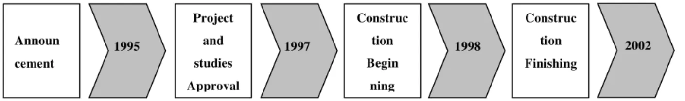
The announcement of Rodoanel was made in January 1995. Mario Covas was then state governor, elected in November 1994. As soon as Covas took office he decided to take up the new beltway project and start its construction. The necessary impact studies were carried out covering all technical, environmental and legal aspects, as well as financial arrangements. The timeline of Rodoanel West Section and the project milestone events are shown in Figure 1.
Figure 1 – Rodoanel West Section Timeline2
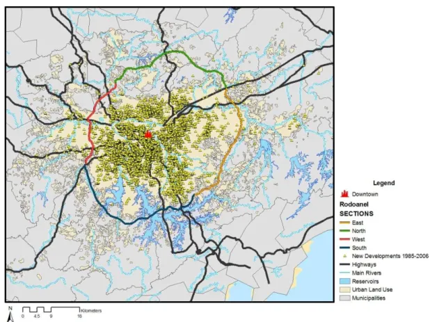
During project preparation, the main concern was the north section. The original route planned would cross the Environmental Protection Area of Serra da Cantareira, which is one of the main water sources for the SPMA (see the green area at the north in Figure 2).
Finally approval was granted for a new planned route in the northern area that avoided any crossings through the Environmental Protection Area of Serra da Cantareira. The strategy to implement the Rodoanel consisted in dividing its construction into four phases—each of them a section. The construction would begin by the western section which was the cheapest and the easiest. The South branch started on 2008 and was recently delivered. The Sao Paulo State is starting the process to build the third branch on the east but it will not resume before the new governor is elected.
2 Source: Secretaria de Estado dos Transportes de São Paulo. Announ
cement
Project
and
studies
Approval
Construc
tion
Begin
ning
Construc
tion
Finishing
Figure 2 – Rodoanel Route (west section detached in red color) 3
We test hypotheses related to two major events: the announcement and the construction of Rodoanel West Section. According to Boarnet and Chalermpong (2001) whose study evaluates new toll roads in Orange County, California, it is important to consider some threshold years and evaluate them because the value of the roads would not be fully capitalized in the announcement or at the beginning of the construction. He notes:
―Even with some foresight on the part of home buyers, we expected that the market
assessment of the likelihood that the roads would be built would rise over the early years
of our data (…).‖ (Boarnet & Chalermpong 2001, pp.581)
2. Hedonic Price Models and Land Use
Hedonic price models have been regularly used in applied studies since the fifties, although they were formally developed in forties (Bartik, 1987). A hedonic price model refers to the demand for a good which encompasses several attributes. Therefore according to Lancaster (1966) the consumer does not buy a single good, but a bundle of different characteristics. Durable goods such as cars or appliances are typical examples. Houses also can be seen as a hedonic good because consumers buy simultaneously location, dimension, and quantity of bedrooms, bathrooms and other characteristics.
Rosen (1974) affirms that consumer‘s utility is obtained by the attributes of the commodity,
not by the commodity itself. As a consequence any good z is expressed as a coordinator vector
z = (z1, z2, …, zn) of its k characteristics. For this reason a hedonic price model is p(z) = f(z1,
z2, …, zn). A simple hedonic price equation is:
k K
k kz z
p
1 0
)
(
Where each attribute zk has a marginal βk impact over p(z), i.e., the marginal price of the characteristic or its implicit value.
According to Bartik (1987) the hedonic price function gives information about the consumer‘s marginal bid for an attribute in a market equilibrium situation. Thus each attribute‘s bid
equals its marginal price. Therefore the hedonic equation is a reduced form of demand and
supply simultaneous interaction system of equations.
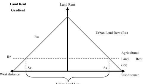
Figure 3 – Land Rent Gradient in a Linear City
One of the attributes of houses is distance from the CBD. This characteristic refers to land use and consequently to land price. Alonso (1960) shows the trade-off between land price and distance from CBD. This trade-off is due to transport costs, which are increasing to distance as represented in Figure 3 for a linear city model.
On the other hand there are negative externalities associated to the new infrastructure. As pointed out by Bouarnet and Chalermpong (2001), the proximity to the lanes (around 500 meters) can bring down house prices. The cause is the noise and air pollution due to the traffic.
So there are two driving forces interacting: accessibility and negative externality. The first helps to increase land prices and the second helps to decrease them. A priori we do not know
which one is greater and where each predominates (around the beltway). Agricultural Land Rent (Rr)
East distance West distance
Land Rent
Land Rent Gradient
Urban Land Use
Urban Land Rent (Ru) Ru
Rr
3. Data
Land prices are not systematic available in datasets. One must look primary for information from field work. One way to deal with this problem is estimate land prices indirectly from house prices. In order to do that we follow Biderman (2001) whose study was the pioneer in using Embraesp (Empresa Brasileira de Estudos Patrimoniais) residential sales database for academic purposes.
Embraesp data cover the SPMA since 1985 and register the asking price only of new residential developments. So these data are not appropriate to evaluate repeated sales as is the usual practice in empirical housing market studies in the US. From 1985 to 2006 there are 10,367 observations in the Embraesp database. 9,460 of them could be geocoded, of which 9,093 have information about the area of the land parcel. It is not a statistical sample stricto
sensu but contains all formal publicly-announced new developments. Thus it can be
representative for some inferences about population. As a consequence our analysis of Rodoanel impacts does not take into account informal markets or commercial developments or re-sales. The Embraesp database contains dwelling-specific information (useful area, quantity of bedrooms and bathrooms etc.).
We incorporate the information on location-specific aspects using block data from the 2000 Census made available by CEM (Centro de Estudos da Metrópole) from CEBRAP (Centro
Brasileiro de Análise e Planejamento). Cheshire and Sheppard (1995, pp. 248) suggest that ‗if
location-specific characteristics of housing are appropriately measured monocentric models
can perform well.‘ So each new residential sale was spatially joined to its 2000 Census block
attributes. The SPMA has more than 17,000 census blocks, each of them with about 400 dwellings units.
4. Hypotheses
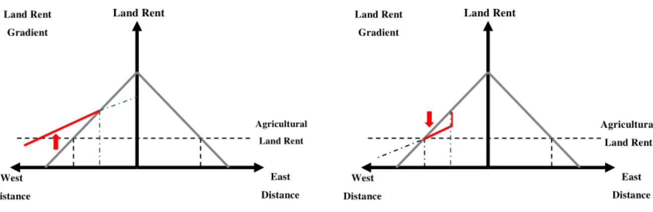
Assuming the monocentric shaped city and the gradient land price according to Alonso (1960), the main hypothesis we test is that Rodoanel West caused increases in land price on the west side of its ramps (Figure 4 – diagram on left). In spite of Rodoanel be focused on cargo transportation, we suspect that its lanes can be adopted for commuting purpose as the traffic jams in SPMA have been increasing and new routes are always looked for.
Conversely, proximity to the lanes may result in negative effects such as noise and air pollution due to traffic. These impacts tend to decrease the land price (Figure 4 – diagram on right).
Figure 4 – Expected Effects on Land Prices after Rodoanel West Section Deployment
In summary, there are two types of effects that are not necessary exclusive: accessibility and negative externalities. We can state the hypothesis in three parts:
(1) Increasing land prices on the ‗outside‘ of the beltway (e.g. accessibility effect
predominates)
0 :
0 :
1 0
ij ij
p H
p H
(2) Decreasing land prices on the vicinity of the beltway‘s lanes (e.g. negative externalities
predominate)
West Distance
East Distance
Land Rent
Agricultural Land Rent
Land Rent Gradient
West Distance
East Distance
Land Rent
Agricultural Land Rent Land Rent
0 : 0 : 1 0 ij ij p H p H
(3) No changes on land prices on the ‗inside‘ of the beltway (e.g. none of the effects
predominate) 0 : 0 : 1 0 ij ij p H p H
(Where pi,j is the residential land price for a dwelling unit i located in zone j)
If our hypothesis is confirmed it will allow us to conclude that those who live outbound of the beltway have an improvement in accessibility, while those who live near the lanes suffer negative effects from traffic, and those who live inbound experience no effect. The consequences for public policy will be several as we discuss further.
5. Research Strategy
We do not want to explore specific situations of Rodoanel West Section such as informal settlements accessibilities or conflicts. We would like to find the average effects of the new highway on land prices related to its announcement and to its construction. So we adopt the traditional econometric methodology for hedonic price estimation.
The first step is to get information about land prices, which is the dependent variable here. Embraesp dataset covers the asking prices of new residential properties, i.e. combines the value of the land and the building in the property asking price. A possible way to obtain land prices is by dividing the asking price of the housing unit(s) by the area of the land parcel area of the parcel where the unit(s) is build.
It is important to mention that these values are in reais (R$) deflated to the year of 2000.
Figure 5 shows the calculated land price histogram.
This measure is imperfect because we do not have the actual cost of production. The implication is the underline assumption of a constant capital-land relation which is a very strong assumption. As we know, the relation capital-land is increasing as we approach the CBD due to higher land prices. If we had the construction costs information the adequate land price could be computed as:
meters square
in area parcel
meters square
in area built . meters
square in area built
costs on constructi
-t developmen new
the of value meters
square Price Land
By using appropriate GIS software4 we calculate the minimum straight-line distance from each new residential unit offered for sale to the downtown center. Such measure is very important, as pointed out by Cheshire and Sheppard (1995), because it brings the urban rent theory approach to the analysis. The theory suggests a trade-off between land price and distance from CBD (e.g. a trade-off between accessibility and transport costs).
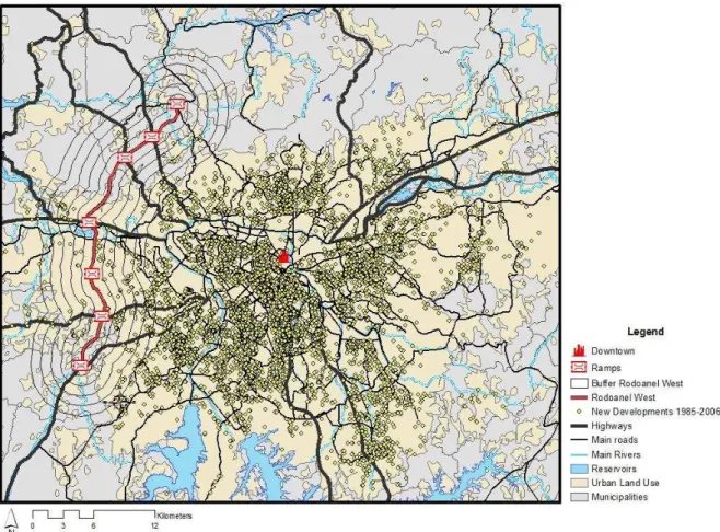
We also calculate the minimum straight-line distance from each new residential unit offered for sale to the Rodoanel West Section‘s lanes and ramps. This allows us to define buffers for
the area of influence of the road and thus the treatment group (see Figure 5).
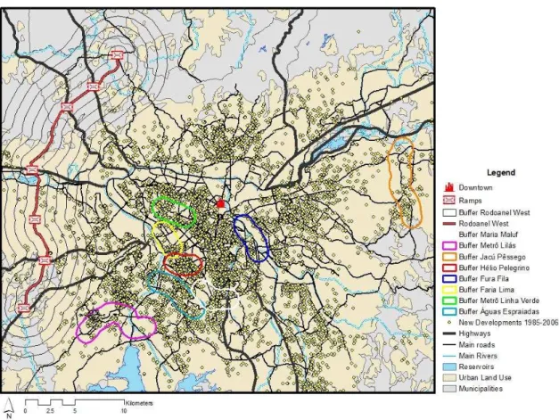
Figure 5 – New residential Developments (1985-2006) and Rodoanel West Section (track, ramps and buffers)5
So we can apply difference-in-differences (‗dif-in-dif‘) technique in order to estimate the impacts caused by Rodoanel West Section. According to Stock and Watson (2003), a basic dif-in-dif specification is:
Where ∆Yi can be considered as the variation on prices for the land parcel i, Xi is the binary variable that informs if the land parcel is surrounding Rodoanel´s ramps and β1 is the causal effect from the deployment of Rodoanel.
5 Source: Embraesp and Centre of Studies of Public Sector Politics and Economics at Getulio Vargas
More specifically we are looking land parcels in the site A affected by Rodoanel. If there is a site B that has not been crossed by Rodoanel, we can use it as a control group to compare the changes between A and B between the two periods (before and after its deployment). So we run the regression:
Where Y is the price of land parcels in each site in each period. T is a time (period) dummy,
SA is a state dummy for site A, and T*SA is the interaction of the period dummy and the site A
dummy. Box 1 displays the hypothetical percentage variation on prices of land parcels in each state and time period and Box 2 explains what each coefficient in the regression represents.
Box 1 – Hypothetical percentage variation on the prices of land parcels
Site A
(surrounding Rodoanel´s ramps)
Site B
(not surrounding Rodoanel´s ramps)
Period 1 (before the deployment
of Rodoanel) b a
Period 2 (after the deployment of
Rodoanel) d c
Box 2 – Calculation and interpretation of regression coefficients
Coefficient Calculation Interpretation
β0 a Baseline average
β1 c − a Time trend in the control
group
β2 b − a Differences between the two
sites in period 1 (before the deployment of Rodoanel)
β3 (d − b) − (c − a) Difference in the changes
over time, e.g. the ‗true‘
impact of Rodoanel.
Each period comprehends a dummy variable which assumes ‗1‘ during the respective stage and ‗0‘ otherwise.
The site specific variables are divided into four groups of dummies. The first group is formed by residential units offered for sale located up to 2,500 meters from Rodoanel‘s ramps
outbound. The second group is obtained in the same fashion but inbound. The third group
captures the residential units offered for sale located beyond 2,500 meters from Rodoanel‘s
ramps outbound. The fourth site specific group stands for the same range of distance from
Rodoanel‘s ramps as the previous but inbound till 5,000 meters.
After matching addresses by condominiums and filtering out inappropriate data (as ‗missing values‘) we are left with 7,392 new dwelling units from 1985 to 2006 with complete range of information. Table 1 summarizes the distribution of observations by interacting site specific and location specific variables. They are the treatment groups and their coefficients represent the net effect of Rodoanel West Section.
Table 1 – Treatment Groups (number of observations)
Interactive Dummies (site*period)
Announcement and Planning
Construction Delivery and Operation
Group 1
(outbound till 2500m)
0 2 8
Group 2
(inbound 2500m)
8 5 14
Group 3
(outbound 2500m)
0 4 42
Group 4
(2500m<inbound<5000m)
12 7 32
But we know there are others factors driving the prices that we must take them into account. Thus our estimator is a kind of dif-in-dif with additional regressors (hedonic price regression).
∑
5.1 Hedonic Price Regression Analysis
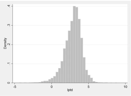
Following the methodology of Boarnet and Chalermpong (2001), Wilson and Frey (2007) and Gatzlaf and Smith (1993) we develop hedonic price regressions.6 However we take into account Cheshire and Sheppard (1995) suggestion that linear forms of the hedonic land price model may have non-normal errors. Therefore we adopt the log-form specification. In addition to support this choice, Figure 6 shows the histogram of the natural logarithm of land prices. The distribution of the logarithm of the prices seems to be closer to the log-normal distribution.
Figure 6 – Histogram of the Natural Log of Square Meter Price of Land
– deflated values (1985-2006)
The model should consider the two groups of factors that drive the land prices as we calculated: dwelling-specific and location-specific factors. Thus the model general specification7 is:
roup4 Delivery .G roup3 Delivery .G roup2 Delivery .G roup1 Delivery .G on.Group4 Constructi on.Group3 Constructi on.Group2 Constructi on.Group1 Constructi nt.Group4 Announceme nt.Group3 Announceme nt.Group2 Announceme nt.Group1 Announceme Group4 Group3 Group2 Group1 Delivery on Constructi nt Announceme Site' nit' Dwelling_U ln 1 9 1 8 1 7 1 6 1 5 1 4 1 3 1 2 1 1 1 0 9 8 7 6 5 4 3 2 10+ + +
= p
Where p = new home sales asking price deflated to 2000 Reais, using the General Price Index
(IGP-DI) for Brazil provided by the Getulio Vargas Foundation; Dwelling_Unit = vector of
dwelling unit characteristics such as size (useful area), number of bedrooms, number of bathrooms, number of parking spaces etc.; and Site = vector of site attributes such as water
system and sewage coverage, head of household average monthly income, dummy for home located in the municipality of São Paulo, straight-line distance from São Paulo downtown.
One option would be to adopt a panel data regression (as ‗fixed effects‘ methodology).
Unfortunately the micro level data are not a true panel. Each new development appears once in the sample (as noted earlier, it is not a repeated-sale database). Even if we aggregate the units for a local average it will be an unbalanced panel, with less degree of freedom. For this reason the use of pooled data and dummies seem to be more appropriate.
Take into account that we want to evaluate the effects of the Rodoanel on surrounding parcels, we have a quasi-experiment. The model that we adopt to estimate the impact of the Rodoanel on the variation of prices from surrounding parcels is a type of dif-in-dif regression. Note that the dependent variable ln(pi) is equivalent to Δpi / pi.
6. Results
We run several regressions changing the control group (see Appendix). In the first regression we considered the full sample and decomposed each time-period described on Figure 1 and each group described on Table 1. The second and the third regressions collapsed the time and site specific dummies in order to look for more general effects. Regressions 4 to 6 constrain the sample to housing located at the same distance from the CBD as the treatment groups.
Almost all control variables are significant at 1 percent and in general have the expected sign. The variables of interest are the interaction between site location (the groups) and the timing. For instance, the interaction between the construction period dummy and group 1 dummy would give us the (counter-factual) impact of the beltway construction on land prices within 2.5 km outbound of the beltway.
The impact of the beltway on land prices is different according to the stage of deployment. The announcement stage brings some positive expectations about benefits, but it is not clear whether they are going to be real. Boarnet and Chalermpong (2001) point out that new highway investments cast doubt on economic agents. Those kinds of investments require huge amounts of resources and face litigations and environmental barriers. Therefore the full values of the roads are not capitalized into land prices until works are completed. In the specific case of Rodoanel West Section the discredit was expressed in non-significant changes in prices. Later on agents can better anticipate benefits and cost.
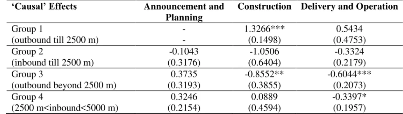
Table 2 – Estimated coefficients and standard errors for selected independent variables from general regression with full sample8
‘Causal’ Effects Announcement and
Planning
Construction Delivery and Operation
Group 1
(outbound till 2500 m)
- -
1.3266*** (0.1498)
0.5434 (0.4753) Group 2
(inbound till 2500 m)
-0.1043 (0.3176)
-1.0506 (0.6404)
-0.3324 (0.2179) Group 3
(outbound beyond 2500 m)
0.3735 (0.3193)
-0.8552** (0.3855)
-0.6044*** (0.2073) Group 4
(2500 m<inbound<5000 m) (0.2154) 0.3246 (0.4594) 0.0889 -0.3397* (0.1957)
The negative impact on Group 3 is the only result that does not changes after delivery and operation. The lack of significance of the delivery suggests that capitalization have happened mainly during construction. In general, the effects for those who live inbound (e.g. closer to the CBD) are not significant. Since it does not make a lot of sense the negative sign we believe that we may be confounding the impacts on areas beyond 2.5 km with some other event that we are not able to control.
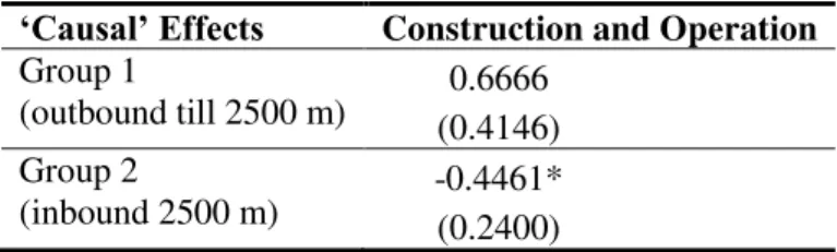
We first collapse the time variable into one major event: the physical presence of the lanes (construction and delivery). This specification reduces the time specific dummies to the
simplest possible form. It assumes ‗0‘ for all periods before construction and ‗1‘after it. The results follow the same general patterns of the decomposed regression. We then omit groups 3 and 4 and concentrate the analysis on Groups 1 and 2.
Table 3 shows the results. Now we are analyzing only the land located near the ramps to Rodoanel outbound and inbound. The results are compatible with the previous ones. Rodoanel West brings accessibility benefits for those who live on the outbound of the lanes but not for those who live on the inbound side. However, the positive effects are non-significant suggesting that the net impact on land prices might have been negative.
Table 3 – Impact of the Rodoanel Construction on Land Price in the Inbound and Outbound Surrounding Areas – Full Sample9
‘Causal’ Effects Construction and Operation
Group 1
(outbound till 2500 m) (0.4146) 0.6666 Group 2
(inbound 2500 m) -0.4461* (0.2400)
We then restrict the geography in order to compare the treatment group with more similar areas. We first impose that the site cannot be in the vicinity of any relevant transportation investment (but the Rodoanel, evidently) built from 1986 to 2006. Thus the number of observations dropped to 5,833 cases. In order to do that, we first identify and segregate other relevant transports investments made during the period. There were several investments but the most important are the following:
The extended subway Green Line which reached Sumaré and Vila Madalena neighborhoods;
The new subway Purple Line in the southern of the city of São Paulo;
The extension of Faria Lima Avenue and the connection to Hélio Pelegrino Avenue;
The initial new lanes for ‗Fura-Fila‘ Bus Rapid Transit (BRT);
The new Águas Espraiadas Avenue;
The interconnection of Bandeirantes Avenue and the ramp to Anchieta Highway
(‗Complexo Maria Maluf‘) – an improvement on the first beltway;
The extension of Jacú-Pêssego Avenue – an improvement on the third projected (and uncompleted) beltway.
Figure 7 – Relevant Transport Investments (buffers), New residential Developments (1985-2006) and Rodoanel West Section (track, ramps and buffers)10
Then we locate these interventions using GIS software. For each intervention we create a buffer of 1.0 km around its track and dropped all new residential developments inside these buffers. The idea is that these cases cannot be considered as a control group since those households have indeed increased their accessibility in the period. The ideal control group would be households that have their accessibility not significantly affected in the period. The interesting result is that now the impact on the outbound sites is significant and it is still positive. The impact on the inbound neighborhood of the road is still significant and negative. These results are confirming the asymmetrical impact of the highway.
10 Source: Embraesp and Centre of Studies of Public Sector Politics and Economics at Getulio Vargas
Table 4 – Impact of the Rodoanel Construction on Land Price in the Inbound and Outbound Surrounding Areas – Sites With no Relevant Investment in Transport11
‘Causal’ Effects Construction and Operation
Group 1
(outbound till 2500 m) (0.4140) 0.7217* Group 2
(inbound till 2500 m) -0.3998* (0.2401)
Figure 8 – Relevant Transport Investments (buffers), New residential Developments which distance from CDB is at least 15.5 km (1985-2006) and Rodoanel West Section (track, ramps and
buffers)12
11 Robust standard errors below coefficients. * p<0.10, ** p<0.05, *** p<0.01.
We then restrict the sample of new developments for which distance from CDB is at least 15.5 km (see Figure 8). This threshold is the closest distance to the CBD from any development in the treatment group. If the rent gradient is changing over time, using the entire sample could imply that we are confounding the impact on the (whole) gradient with the impact of the road. Concentrating on the same distance from the CBD would allow to control for such possible pattern.
As we can see the impact of Rodoanel‘s is still significant for the prices of Groups 1. For
Group 2 the impact are still positive but not significant.
Table 5 – Impact of the Rodoanel Construction on Land Price in the Inbound and Outbound Surrounding Areas – Sites with no Relevant Investment in Transport and more than 15.5km far
from the CBD13
‘Causal’ Effects Construction and Operation
Group 1
(outbound till 2500 m) 0.9496** (0.4317) Group 2
(inbound till 2500 m) (0.2831) 0.3357
Finally we drop from the analysis the new residential developments located up to 1km from the lanes. This follows a similar procedure used by Boarnet and Chalermpong (2001) in order to deal with noise and air pollution externalities from the traffic. With this new restriction we end up with 493 observations.
As we can see the in Table 6, the impact of Rodoanel‘s operation is again positive on the prices of Groups 1 and 2, but it is significant just for the first one. The sign and significance are exactly the same found in the previous regression and the magnitude of the coefficients is very similar to the previous specification. Thus it seems that the eventual negative effects of being near the lanes are not stronger enough to overcome the benefits of accessibility.
Table 6 – Impact of the Rodoanel Construction on Land Price in its Inbound and Outbound Surrounding Areas – Sites with no Relevant Investment in Transport, more than 15.5km far
from the CBD and more than 1km far from the Rodoanel 14
‘Causal’ Effects Construction and Operation
Group 1
(outbound till 2500 m) (0.4701) 0.9084* Group 1
(outbound till 2500 m) (0.3578) 0.3177
We summarize the statistically significant findings in Table 7 in order to bring about better and clear synthesis.
Table 7 – Variations on housing land parcels caused by Rodoanel West Section
Compared to the rest of the land parcels of SPMA
Compared to the rest of the land parcels of SPMA
(collapsing time variables into one major event:
construction and delivery)
Compared to sites with no relevant investment in transport
Compared to sites with no relevant investment in transport and more than 15.5km far from the CBD
Compared to sites with no relevant investment in transport, more than 15.5km far from the CBD and more than 1km far from the Rodoanel
Group 1 (outbound till 2500 m)
133% during construction
- 72% during deployment
95% during deployment
91% during deployment
Group 2 (inbound till 2500 m)
- -45% during
deployment -40% deployment during - -
If we read the different estimations ‗backwards‘ we will note the general nature of the
asymmetrical effects of Rodoanel:
1) Residential land parcels around the track of Rodoanel have negative or null price changes depending on the different sides from its lanes and the different distances from its ramps (when compared to more restricted comparison groups – e.g. similar characteristics but distant from any relevant transport intervention and/or equally distant from CBD).
2) The different periods of deployment have different effects on land prices. Rodoanel is a huge infrastructure project that took seven years from the announcement to the beginning of operations for its first section. If we do not take this into account we will misunderstand how Rodoanel has affected land prices.
3) Residential land parcels around the track of Rodoanel have negative or null or positive price changes depending on the different sides from its lanes and the different distances from its ramps (when compared to less restricted comparison groups).
In short, the results obtained by the econometric models show an asymmetric effect of Rodoanel on land prices. Let us take the last specification as the ultimate specification to be tested in order to discuss these results (see the last column on Table 7). Although the results corroborate the general hypothesis of asymmetry, there are some specific differences highlighted in Box 3.
Box 3 – Expected versus Estimated Effects: conclusions15
Original Hypothesis Conclusion
Increasing land prices on the ‗outside‘ of the beltway (e.g. accessibility effect predominates)
The effects are significant and positive for residential land parcels closer to the Rodoanel‘s ramps*.
Decreasing land prices on the vicinity of the beltway‘s lanes (e.g. negative externalities predominate)
The negative externality from closer proximity seems to be not significant (at least for the new residential developments).
No changes on land prices inbound the beltway (e.g. none of the effects predominate)
The effects are not significant (statistically null) for residential land parcels closer to Rodoanel‘s ramps**.
15 * For parcels which are located farther (beyond 2.5 km) the effects are not significant (statistically
Figure 9 shows a schematic representation of the result found: a kinked land rent gradient which is below the former land rent gradient for residential land parcels located on the right side of the ramps to the lanes and it is above the former land rent gradient for residential land parcels located up to 2.5 km on the left from the ramps to the lanes. The latter are those who really seem to obtain commuting benefits from the beltway. It should be noticed that there were no significant improvement in commuting alternatives (such as bus and commuter rail) along the west side of SPMA during the period evaluated.
Figure 9 – Illustration of the Results from Hedonic Price Equation (last specification)
These short-run effects tend to vanish over the years as residential and commercial location decisions are made. Also the better level of commuting service brought by Rodoanel will tend to diminish as the demand for the beltway goes up. Whereas changes on density seem to be plausible around the new beltway, there is no reason to believe that it can have enough power to contribute to increasing urban sprawl.
These findings would suggest taxation possibilities for purposes of urban policy. The economic rent created by Rodoanel could be taxed to fund the next section of the beltway or to cover its operational expenses. On the other hand if a tax is levied, that could reduce any advantage for new residential developments located far from the CBD.
The problem is that property taxes in Brazil are the responsibility of municipalities and the Rodoanel investment is funded by the state and the national government. Moreover, the eventual capturing of the incremental land value through property tax and the corresponding
West Distance
Land Rent
Agricultural Land Rent
East Distance
Land Rent Gradient
15km 22.5km 20 km
Rodoanel West
increase in municipal tax revenue can only be realized by the municipalities on the west of the beltway since, as we have seen, parcels on the east side experienced a decline in land values. Consequently the municipality of São Paulo, located on the east side of the beltway, would face a decline in property tax revenues from parcels located near the beltway.
The appropriation for commuting use of a road designed for cargo traffic, as is the case of Rodoanel, and the potential rent generated by this behavior is reflected in the congestion observed near the intersections of the beltway with radial highways in the peak-hours. That is one of the reasons why São Paulo state government was motivated to implement tolls on the ramps to Rodoanel West Section in the beginning of 2009.
Conclusion
This paper shows the findings from a research about the impact of the West Section of the Rodoanel beltway on land prices. We evaluate road announcement, construction and delivery/operation events. The results of the econometric methods used show that there are significant and asymmetrical effects attributed to Rodoanel.
The Roadanel construction and delivery/operation increase land prices of parcels located closer to ramps on the west side of the track. The connection between the beltway and the radial highways may be providing new commuting routes to the São Paulo CBD.
For parcels located on the east side of the beltway, relatively far from the track (between 2.5 km and 5 km), the effects of construction and delivery/operation have the opposite effect: these parcels face a decline in land prices.
References
Alonso, W. (1960) Theory of urban land market. Papers and Proceedings of Regional Science Association, vol. 6, pp. 149-157.
Bartik, T. (1987) The estimation of demand parameters in hedonic price models. Journal of Political Economy, vol. 95, n. 11, pp. 81-88.
Becker, S. O. and Ishino, A. (2002) Estimation of average treatment effects based based on propensity score. The Stata Journal, vol. 2, n. 4, pp. 358-377.
Biderman, C. (2001) Forças de atração e expulsão na Grande São Paulo. Tese de Doutorado Apresentada ao Curso de Pós Graduação da EAESP/FGV. São Paulo: EAESP/FGV.
Bouarnet, M. G. and Charlermpong, S. (2001) New highways, house Prices, and urban development: a case study of toll roads in Orange County, CA. Housing Policy Debate, vol. 12, n. 3, pp.
575-605.
Chesschire, P. and Sheppard, S. (1995) On the price of land and the value of amenities. Economica,
vol. 62, n. 246, pp. 247-267.
Epple, D. (1987) Hedonic prices and implicit markets: estimating demand and supply functions for differentiated products. Journal of Political Economy, vol. 95, n. 11, pp. 59-80.
Gatzlaff, D. H. and Smith, M. T. (1993) The impact of Miami metrorail on the value of residences near station locations. Land Economics, vol. 69, n. 1, pp. 54-66.
Lanchaster, K. J. (1966) A new approach to consumer theory. Journal of Political Economy, vol. 74,
n. 2, pp. 132-157.
Meyer, R., Grostein, M. and Biderman, C. (2004) São Paulo metrópole. São Paulo: EDUSP.
Prestes Maia, F. (1930) Plano de avenidas. São Paulo: Melhoramentos.
Rosen, S. (1974) Hedonic prices and implicit markets: product differentiation in pure competition,
Journal of Political Economy, vol. 82, pp. 34-55.
Stock, J. H. and Watson, M. W. (2003) Introduction to econometrics. Addison Wesley.
Wheaton, W. (1977) Residential decentralization, land rents and the benefits of urban transportation.
American Economic Review, vol. 67, n. 2, pp. 138-145.
Wilson, B. and Frew, J. (2007) Apartment rents and locations in Portland, Oregon: 1992-2002.
Appendix
Table 8 – Estimation results16
Var. Dep.: Ln (p) Regression
1 Regression 2 Regression 3 Regression 4 Regression 5 Regression 6
Constant 6.3157*** 6.3392*** 6.3676*** 6.2731*** 14.4167*** 14.1118***
(0.3160) (0.3137) (0.3145) (0.3448) (2.6929) (2.6959) ln of useful area -0.6868*** -0.6356*** -0.6354*** -0.6186*** -0.8842*** -0.8854***
(0.0468) (0.0470) (0.0474) (0.0527) (0.2068) (0.2063) # of bedrooms -0.0766*** -0.0920*** -0.0932*** -0.0757*** -0.0660 -0.0933
(0.0212) (0.0216) (0.0216) (0.0245) (0.1062) (0.1082)
# of bathrooms 0.1537*** 0.1428*** 0.1436*** 0.1189*** 0.3130*** 0.3299***
(0.0225) (0.0229) (0.0230) (0.0257) (0.0922) (0.0940)
# of parking places -0.0085 -0.0264 -0.0262 -0.0332 -0.1493* -0.1427*
(0.0195) (0.0196) (0.0197) (0.0220) (0.0809) (0.0808)
# of elevators -0.0011 -0.0031 -0.0025 -0.0008 0.1108*** 0.1152***
(0.0058) (0.0061) (0.0061) (0.0073) (0.0342) (0.0348)
# of floors 0.0639*** 0.0654*** 0.0658*** 0.0654*** 0.0507*** 0.0498***
(0.0019) (0.0020) (0.0020) (0.0023) (0.0102) (0.0104)
penthouse 0.0322*** 0.0362*** 0.0365*** 0.0328*** 0.0491* 0.0496*
(0.0062) (0.0064) (0.0064) (0.0070) (0.0276) (0.0284) percentage of dwellings with sewage coverage -0.1092 -0.1575 -0.1638 -0.2035 -0.2684 -0.2683
(0.1166) (0.1225) (0.1191) (0.1289) (0.2079) (0.2070) percentage of dwellings without bathrooms -1.8126 -1.6787 -1.8362 -0.5558 -6.4494 -7.8416
(2.0933) (2.1472) (2.1507) (2.1785) (6.2692) (6.6370) percentage of dwellings with garbage services coverage 0.0884 0.0690 0.0611 0.1577 0.9216 0.8895
(0.1520) (0.1503) (0.1501) (0.1582) (0.6683) (0.6738) percentage of dwellings with water system coverage 0.0722 -0.0136 0.0068 0.0261 -0.7474 -0.7903
(0.2516) (0.2559) (0.2565) (0.2730) (0.7173) (0.7231)
ln of income 0.0071 -0.0080 -0.0034 -0.0123 -0.0936 -0.0757
(0.0153) (0.0113) (0.0113) (0.0132) (0.0738) (0.0769) ln of population density in sector -0.0355*** -0.0388*** -0.0414*** -0.0414*** -0.0399 -0.0299
(0.0121) (0.0124) (0.0123) (0.0138) (0.0539) (0.0543) municipality of Sao Paulo 0.1062*** 0.1416*** 0.1717*** 0.1783*** 0.1209 0.1608
(0.0295) (0.0300) (0.0295) (0.0324) (0.1213) (0.1299) ln of distance from Sao Paulo downtown -0.0619*** -0.0623*** -0.0714*** -0.0695*** -0.7316*** -0.7145***
(0.0118) (0.0118) (0.0118) (0.0124) (0.2167) (0.2167) Rodoanel west section: announcement -0.3021***
(0.0285) Rodoanel west section: construction -0.3780***
(0.0357) Rodoanel west section: delivery -0.7116***
Table 8 – Estimation results (cont.)
Var. Dep.: Ln (p) Regression
1 Regression 2 Regression 3 Regression 4 Regression 5 Regression 6 (cont.)
near till 2500m west from Rodoanel -2.3469*** -2.3013*** -2.2954*** -2.3141*** -2.3443*** -2.3399*** (0.1355) (0.1329) (0.1388) (0.1402) (0.2155) (0.2209) near till 2500m east from Rodoanel 0.1421 0.0540 0.0694 0.0603 -0.3879 -0.6101* (0.1933) (0.1588) (0.1588) (0.1607) (0.2436) (0.3536) near beyond 2500m west from Rodoanel -0.0254 0.0174
(0.1677) (0.1667) near between 2500m and 5000m east from Rodoanel -0.1670 -0.0905
(0.1313) (0.1111) announcement*proximity 2500m west 0.0000
(0.0000) announcement*proximity 2500m east -0.1043
(0.3176) announcement*proximity beyond 2500m west 0.0000
(0.0000) announcement*proximity 2500m-5000m east 0.3246
(0.2154) construction*proximity 2500m west 1.3266***
(0.1498) construction*proximity 2500m east -1.0506
(0.6404) construction*proximity beyond 2500m west -0.8552**
(0.3855) construction*proximity 2500m-5000m east 0.0889
(0.4594)
delivery*proximity 2500m west 0.5434
(0.4753)
delivery*proximity 2500m east -0.3324
(0.2179) delivery*proximity beyond 2500m west -0.6044***
(0.2073) delivery*proximity 2500m-5000m east -0.3397* (0.1957)
after construction has started -0.5047*** -0.5143*** -0.5610*** -0.9013*** -0.8750*** (0.0227) (0.0226) (0.0252) (0.1535) (0.1613)
after*proximity 2500m east -0.4671* -0.4461* -0.3998* 0.3357 0.3177
(0.2407) (0.2400) (0.2401) (0.2831) (0.3578)
after*proximity 2500m-5000m east -0.3889**
(0.1871)
after*proximity 2500m west 0.6227 0.6666 0.7217* 0.9496** 0.9084*
(0.4133) (0.4146) (0.4140) (0.4317) (0.4701)
after*proximity beyond 2500m west -0.7335***
(0.2031)
R-squared 0.43 0.41 0.40 0.42 0.58 0.58