Abstract
The analytical approach is presented for both symmetric and anti-symmetric local buckling of the thin-plate in finite sizes and with a center crack under tension. An efficient classical solution based on the principle of minimum total potential energy was provided using only 2 and 1 degrees of freedom for symmetric and anti-symmetric modes and the linear elas-tic buckling loads are evaluated by the means of Rayleigh-Ritz method. In the pre-buckling state, a correction factor for the peak compressive stress in the finite cracked plates is defined with an empirical formula and used in the analytical solution of the buckling. To verify the analytical approach, a wide range of numerical results by aid of finite element method are provided herein and a comparison between theo-retical results with the experimental work of other research-ers has been done. Both numerical and experimental results accept the accuracy and validity of the presented analytical model.
Keywords
Cracked plate; tension; linear elastic buckling; Rayleigh-Ritz method.
An efficient analytical model to evaluate the first two local
buckling modes of finite cracked plate under tension
1 INTRODUCTION
In a cracked plate subjected to the tension load, perpendicular to the crack orientation, the developed compressive stress near the crack leads to buckling of crack edges. This phenomenon which can be called as local buckling of cracked plates under tension, has been studied by numerous researchers. The early works were the experimental studies such as the Air Force Flight Dynamics Laboratory (AFFDL) results in AFFDL-TR-65-146 (1965); Zielsdorff and Carlson (1972). Similarly, Dyshel (1990; 1999; 2002) has presented some variety of experimental results on the stability and fracture of plate with a central crack referred to as a non-classical problem.
Ali Ehsan Seifa
Mohammad Zaman Kabirb*
aDepartment of Civil Engineering,
Amirkabir University of Technology (Teh-ran Polytechnic), Hafez Street, Teh(Teh-ran, Iran.
bProfessor, Head of the Department of Civil
Engineering, Amirkabir University of Tech-nology (Tehran Polytechnic), Hafez Street, Tehran, Iran.
Tel: +9821-64543016
Corresponding author: b*[email protected]
http://dx.doi.org/10.1590/1679-78251773
Latin American Journal of Solids and Structures 12 (2015) 2078-2093
Besides, the numerical techniques such as the finite element method (FEM) have been carried out by many investigators such as Markstrom and Storakers (1980); Sih and Lee (1986); Shaw and Huang (1990); Brighenti (2005a; 2009) to evaluate the critical load in various geometry and boundary con-ditions. Furthermore, Riks et al. (1992) studied the buckling and the post-buckling behavior from the viewpoints of stability and fracture mechanics by the aid of finite element method.
As Cherepanov (1963) mentioned, an analytical solution for this problem is engaged to some mathematical and fundamental difficulties because the exact solution for in-plane fields of stress and displacement exists just for the infinite plates and mathematically it is complex as well as the local buckling shapes. Guz et al. (2004) presented an analytical solution for the buckling of infinite cracked plate under tension. For the finite cracked plate, Brighenti (2005b) used an approximate model with estimated pre-buckling stress functions. In that work, the stress functions are in the form of hyperbolic series with infinite terms. The buckling shape function is considered to be a radial Gauss-like function (same function of x and y) in which the values of the two unknown parameters were assumed by the author. Both Guz et al. (2004) and Brighenti (2005b) consider the first mode of buckling, which is called the symmetric mode.
Following the previous studies, the most of non-experimental works concern the numerical studies which use many degrees of freedom to solve the problem. Against, the current paper intends to present an efficient classical solution for the non-classical problem of the central cracked plate buckling under tension, which includes only 2 and 1 degrees of freedom for both first (symmetric) and second (anti-symmetric) modes of buckling and has answer for the finite plates with various geometric ratios. In this direction, primarily, the pre-buckling stress state is approximated by a simple function and then the proper shape functions with minimum degrees of freedom are used to describe the buckling mode shapes. Finally, the total potential energy is written as a function of the pre-buckling stress and the buckling deflection and subsequently, the well-known Rayleigh-Ritz method is used to evaluate the critical loads for each mode of buckling. All results were validated with several numerical finite ele-ment simulations in ABAQUS environele-ment and some existing experiele-mental works.
2 ANALYTICAL APPROACH
2.1 General considerations
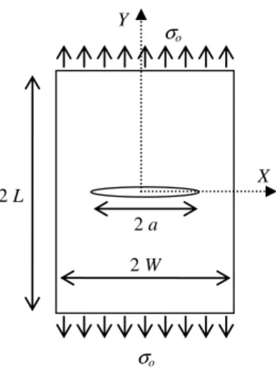
Figure 1 shows the finite cracked plate, with the thickness t, under tension load. The geometric parameters are shown in this figure as well. As shown, the central crack orientation is perpendicular to the load direction which corresponds to the lowest buckling load and in terms of geometry it has two axes of symmetry consistent with the X and Y .
It is assumed that the material is isotropic and linearly elastic with Young’s modulus E and Poisson’s ratio ν. Since σij denotes the pre-buckling stresses, from Von Karman’s linearized theory, the total potential energy Π is obtained based on the transverse displacement w x y
( )
, as the following equation:(
)(
)
(
)
2 2 2 2 2
, , 2 1 , , , , 2 , , , d d
2 xx yy xx yy xy x x xy x y y y
D t
w w w w w w w w w x y
D
ν σ σ σ
Π = + − − − − + +
∫∫
(1)Latin American Journal of Solids and Structures 12 (2015) 2078-2093 Figure 1: The finite plate with a central crack under tension.
By minimizing the total potential energy, ∂Π =0, the critical load can be obtained from an
Eigen-value problem. In Figure 2, the first and second modes are shown in which the buckling deformations are symmetric w x
(
,−y)
=w x y( )
, and anti-symmetric w x(
,−y)
= −w x y( )
, . Given that X and Y are two axes of symmetry, it is possible to consider only a quarter of the plate in the analytical model.
Figure 2: Symmetric and anti-symmetric buckling modes.
As can be seen, the maximum deflection occurs at the center of the crack for both modes and gener-ally, the deformations are insignificant in the regions away from the crack, because the instability of the crack edges is a local buckling phenomenon due to the compressive stress near the crack. Thus, providing a mathematical solution to this problem requires reviewing and determining the status of pre-buckling stress and especially compressive stress along the crack edges.
2.2 Pre-buckling stress state
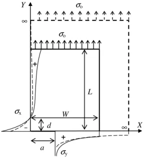
The exact solution for the stress field of an infinite plate with a crack under the in-plane loads exists in many references such as Sadd (2005) but for the finite plates, due to the complexity of the problem, it cannot achieve such relations. In Figure 3, the distribution of stresses σx and σy on the axes X and Y of a finite cracked plate schematically are compared with the infinite one under the same tension stress σo.
It is necessary to note that due to the symmetry, the tangential stress on the symmetry axes is zero and just normal stress exists. In this model, the normal stress σx acting on the Y -axis includes
2 a
σo
σo
X Y
Latin American Journal of Solids and Structures 12 (2015) 2078-2093
the local compressive stress parallel to the crack edges that is the main reason for the local buckling and should be considered in the analysis.
For some finite cracked plates problems, infinite plate relations can be used with some simplifica-tions such as applying a correction factor related to the finite size of the plate. For example, in the field of fracture mechanics, the correction factor β is used for the singular stress field at the crack tip of the finite plates. The values of β can be assessed using numerical methods and for different
geometric ratios a W , L W are presented in Isida (1971). In this study, another correction factor β′
is defined and used for the peak compressive stress. From the exact solution of infinite cracked plate under tension in Sadd (2005), the stress distribution σx on the axis Y is obtained as follows:
(
)
(
)
(
)
2 2
3 2 2
2
0, 1
1
x x o
Y a Y
Y
Y
σ σ σ
+
= = −
+
(2)
According to the equation (2), the maximum compressive stress is obtained for Y =0 which the value is equal to the applied tensile stress σo. So by using the correction factor β′, the peak
com-pressive stress for the finite cracked plate is achieved as β′ ×σo. In section 3.1, the values of β′ are
obtained for different ratios a W , L W using the finite element method.
2.3 Simplified analytical model
A simple analytical model that is used to estimate the buckling load of the finite cracked plate is shown in Figure 4. It is clear that one quarter of the plate is considered and the distribution of the stress σx on the Y -axis is represented as a simple bilinear function.
Figure 3: Comparison of stress distribution in the one quarter of a finite cracked plate (solid line) and the infi-nite one (dash line) under same tension. (+) for tensile
and (-) for compressive stresses.
Figure 4: Simplified model of the finite cracked plate. +
a
X Y
W L
σx
σy + −
−− −
σo
σo
∞ ∞
d
a
X
Y
W
−
a
L
σ
cσ
td
2
1
Latin American Journal of Solids and Structures 12 (2015) 2078-2093
For both finite and infinite cracked plates, the stress σx along Y -axis changes from a negative value to a positive one and at a special point (e.g. Y =d) it is zero (see Figure 3). From equation (2), the zero-value location d for the infinite plate can be found by setting σx = 0 which results in
5 1 0.8 2
d =a − ≈ a (3)
It is assumed that the value of d depends only on the crack length so that the constant δ =d a ≈0.8 can be defined and used for the finite plate with arbitrary dimensions as shown in Figure 4. This assumption is further verified in section 4.1. Now, using dimensionless parameters y =Y a and
L a
=
ℓ , the simple bi-linear function
x
σ with the value of −σc at y =0, σt at y =ℓ and zero for
y =δ can be written as
if 0 1 1 if c x t y y y y δ σ δ σ δ σ δ δ δ
− − < <
=
− − < <
− ℓ ℓ (4)
In the bi-linear function, σc is the peak compressive stress and can be achieved as σc = ×η σo, where
η equals β′ multiplied by a reduction coefficient C related to the linearization of σx. In this study,
roughly C =0.9 is used for all analytical cases but the exact value can be set by a regression analysis on the results. Apart from that, using the force equilibrium along the X direction, σt value is ob-tained in terms of the variable σc according to the following equation.
t c δ σ σ δ =
ℓ− (5)
Finally, equation (4) is rewritten as follows.
2
0.9 1 if 0
if 0.9 1 o x o y y y y
β σ δ
δ σ δ δ β σ δ δ
− ′ − < <
=
− ′ − < < − ℓ ℓ (6)
Latin American Journal of Solids and Structures 12 (2015) 2078-2093
(
)
( ) ( )
( ) ( )
( ) ( )
1 1 2 2
3 2
if 0 1 ,
if 1
o
o
x
w f x g y f x g y
w x y
x
w f x g y ω
+ ≤ ≤
= ≤ ≤
(7)
in which w0 =w
( )
0, 0 is the maximum deflection and(
) (
2)
2(
)
(
)(
)
1 2 3
1 2
1 1 3 ; 1 ; 1
1 ; 1 1
2
x x x
y y
f e x x f e Ax x f e B x x
y y y y
g e g e
ω
− − −
− −
= − + = − = − −
= − = − + +
ℓ ℓ ℓ
(8)
where A is an arbitrary parameter and a continuing condition at x =1 leads to B =A
(
ω−1)
. In this case, the division line x =1 acts as a simple support. It is necessary to note that these functions are obtained through multiplying an exponential decay that exerts locally the nature of buckling, to polynomial functions so that the overall satisfies all conditions in Table 1.Buckling Mode Panel Left Right Top Bottom
Symmetric 1 ,
0
x
w = w ≈0 w= 0 w,y ≠0
2 w ≈ 0 w= 0 w= 0 w,y =0
Anti-symmetric 1 w,x =0 w ≈0 w= 0 w,y ≠0
2 w ≈ 0 w= 0 w= 0 w= 0
Table 1: Boundary conditions of buckling shape modes at panels’ edges.
From Table 1, it is clear that for the anti-symmetric mode, the panel 2 has four edges with zero deflection and it is not unreasonable to assume w x y
( )
, =0 for 1≤ ≤x ω. In other words, thedivi-sion line x =1 acts as a clamped support. This assumption simplifies the solution for anti-symmetric
mode so that the shape function can be lessen as
(
)
4( ) ( )
13 2
4
, 0 1
2 3 1
o
w x y w f x g y x
f x x
= ≤ ≤
= − + (9)
To calculate the potential of applied stresses σx and σo shown in Figure 4, the first assumption is
that the stress σx acts throughout the horizontal shortening (in X-direction) due to the buckling deflection of panel 1. For the stress σo which acts in the vertical direction (Y -direction), since the crack edge is free to move, the vertical shortening due to the buckling deflection appears as crack mouse opening. Consequently it can be assumed that the stress σo is relatively without moving so
that the related potential can be neglected in the analysis.
Latin American Journal of Solids and Structures 12 (2015) 2078-2093 3 EVALUATIONS USING FEM
A wide range of models were prepared in ABAQUS environment in order to determine the correction factor β′ and numerical evaluation of the buckling loads in which the effect of parameter L W, which so far has received less attention, is also included.
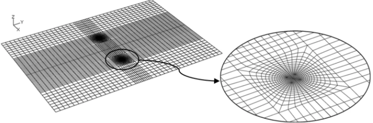
After some mesh size sensitivity analysis with relation to the buckling load, the proper finite element mesh with adequate refinement near the crack tips is illustrated in Figure 5 in which, 4-node doubly curved general-purpose shell elements S4R have been used.
Figure 5: Typical finite element mesh and crack tip detail.
3.1 Peak compressive stress correction factor
In section 2.2, the correction factor β′ was defined for the peak compressive stress in the finite plates
under tension as that amount can be calculated using the finite element models. Given that the pre-buckling stress field is independent of the material properties, the β′ is only related to the geometry
of the plate. Therefore, several models have been developed with different aspect ratios a W = 0.2 ∼0.5 and L W =1∼2, the results are presented in Table 2.
a W L W =1 1.25 1.5 1.75 2.0
0.00 1.0000 1.0000 1.0000 1.0000 1.0000 0.20 1.0676 1.0409 1.0270 1.0212 1.0191 0.25 1.1148 1.0719 1.0500 1.0409 1.0377 0.30 1.1730 1.1093 1.0775 1.0644 1.0598 0.35 1.2433 1.1536 1.1098 1.0920 1.0858 0.40 1.3264 1.2052 1.1475 1.1243 1.1163 0.45 1.4231 1.2645 1.1908 1.1616 1.1516 0.50 1.5339 1.3317 1.2402 1.2044 1.1922
Table 2: β′ for different aspect ratios from FEM.
Like the infinite cracked plates, the value of β′ for small cracks in comparison with plate dimensions
Latin American Journal of Solids and Structures 12 (2015) 2078-2093
Due to the use of β′ in the proposed solution, it will be useful to determine an approximate
formula for β′ based on the numerical results. Using the method of separation of variables, the
general form of β′ can be considered as follows.
(
) (
)
1 F a W G L W
β′ = + (10)
Each of the functions F and G has certain limit values which are useful to determine their overall form. For example, by changing a W from 0 to 1, F a W
(
)
must change from 0 to infinityrespec-tively and similarly G L W
(
)
changes from infinity to 1 when L W changes from 0 to infinity. Due to the described conditions, several functions were considered for F and G and they were analyzed using numerical results and applying least squares method. Finally, appropriate forms of the functionsF and G are recommended below.
(
)
(
)
(
)
2
2
2 1
a W F a W
a W
= −
(11)
(
)
(
)
38
1 1.3
3
G L W
L W
= + ≥ (12)
Due to the simple form and precision of the defined formula for β′, it can very well be used in the
analytical solution presented in section 2.
3.2 Buckling loads for the symmetric and anti-symmetric modes
Using equation (1) with the Rayleigh-Ritz method, it can be easily shown that the buckling load is directly related to the elastic modulus E and inversely with t2 (the thickness to the power of 2).
Thus, the other parameters involved in the problem are the crack length a, the dimensions of the plate L, W and the Poisson's ratio ν that their influence must be evaluated on the buckling load.
For this purpose, finite element models have been developed with different Poisson's ratios ν =
0.1∼0.4 and the aspect ratios a W =0.2∼0.5, L W =1∼2 and the values of buckling load are presented in Table 3 as the dimensionless quantities. It should be noted that in these models, the constant parameters are E =200 GPa, t =1 mm, W =200 mm and all exterior edges are considered to be simply supported. These results are used to validate the analytical results and are discussed in section 4.
4 VERIFICATION AND DISCUSSION OF THE RESULTS
4.1 Pre-buckling stress distribution and the correction factor β′
In Figure 6, the curves of correction factor β′ from equation (10) are drawn for the different ratios
Latin American Journal of Solids and Structures 12 (2015) 2078-2093 3
10
cr E
σ ×
0.1
ν =
Symmetric mode Anti-symmetric mode
a W L W =1 1.25 1.50 1.75 2.0 L W =1 1.25 1.50 1.75 2.0 0.20 0.911 0.930 0.947 0.954 0.956 1.257 1.298 1.324 1.337 1.341 0.25 0.563 0.582 0.597 0.605 0.608 0.768 0.804 0.828 0.840 0.844 0.30 0.376 0.394 0.409 0.417 0.419 0.505 0.538 0.560 0.570 0.574 0.35 0.267 0.283 0.297 0.304 0.306 0.350 0.379 0.399 0.408 0.412 0.40 0.197 0.212 0.224 0.230 0.232 0.253 0.278 0.295 0.304 0.307 0.45 0.151 0.164 0.175 0.179 0.180 0.188 0.210 0.225 0.233 0.236 0.50 0.118 0.130 0.139 0.142 0.143 0.144 0.163 0.176 0.183 0.186
0.2
ν =
Symmetric mode Anti-symmetric mode
a W L W =1 1.25 1.50 1.75 2.0 L W =1 1.25 1.50 1.75 2.0 0.20 0.887 0.906 0.922 0.929 0.931 1.231 1.271 1.297 1.309 1.313 0.25 0.548 0.567 0.582 0.590 0.592 0.752 0.788 0.811 0.822 0.827 0.30 0.367 0.384 0.399 0.406 0.408 0.495 0.527 0.548 0.559 0.562 0.35 0.260 0.276 0.289 0.296 0.298 0.343 0.371 0.391 0.400 0.404 0.40 0.192 0.207 0.219 0.224 0.225 0.248 0.272 0.289 0.298 0.301 0.45 0.147 0.160 0.170 0.175 0.175 0.184 0.206 0.221 0.228 0.231 0.50 0.115 0.127 0.135 0.138 0.139 0.141 0.159 0.173 0.179 0.182
0.3
ν =
Symmetric mode Anti-symmetric mode
a W L W =1 1.25 1.50 1.75 2.0 L W =1 1.25 1.50 1.75 2.0 0.20 0.873 0.892 0.907 0.914 0.916 1.217 1.256 1.281 1.293 1.298 0.25 0.540 0.558 0.573 0.581 0.583 0.744 0.779 0.802 0.813 0.818 0.30 0.361 0.379 0.393 0.400 0.402 0.490 0.521 0.542 0.552 0.556 0.35 0.256 0.272 0.285 0.291 0.293 0.340 0.367 0.386 0.395 0.399 0.40 0.189 0.204 0.216 0.221 0.222 0.245 0.267 0.286 0.294 0.298 0.45 0.147 0.158 0.167 0.172 0.172 0.184 0.203 0.218 0.226 0.229 0.50 0.113 0.124 0.133 0.136 0.136 0.139 0.158 0.171 0.177 0.180
0.4
ν =
Symmetric mode Anti-symmetric mode
a W L W =1 1.25 1.50 1.75 2.0 L W =1 1.25 1.50 1.75 2.0 0.20 0.869 0.888 0.903 0.910 0.912 1.215 1.254 1.278 1.290 1.294 0.25 0.537 0.556 0.571 0.578 0.580 0.743 0.778 0.800 0.811 0.815 0.30 0.360 0.378 0.392 0.399 0.401 0.489 0.520 0.541 0.551 0.555 0.35 0.255 0.272 0.284 0.290 0.292 0.339 0.367 0.386 0.395 0.398 0.40 0.189 0.204 0.215 0.220 0.221 0.245 0.269 0.286 0.294 0.297 0.45 0.144 0.157 0.167 0.171 0.171 0.182 0.203 0.218 0.225 0.228 0.50 0.112 0.124 0.132 0.135 0.134 0.139 0.157 0.170 0.177 0.179
Latin American Journal of Solids and Structures 12 (2015) 2078-2093
Figure 6: Correction factor β′ as a function of a W and L W from equation (10) and FEM from Table 2.
Figure 6 shows that, the approximate equation (10) for β′ is in good agreement with the finite
element results so that the maximum difference is less than 1.5 % in all cases. Also, by changing any of the parameters a W and L W, the FEM results will follow the expected and defined trend for β′
function. For example, with decreasing a W , the value of β′ decreases and approaches to 1 for all
ratios of L W.
Overall, the curves in Figure 6 show the effect of plate dimensions and the crack length on the peak compressive stress, so that, the peak compressive stress increases with increasing the crack length and decreasing the length of the plate in comparison with plate width.
Apart from the correction factor β′, Figure 7 shows the normalized actual distribution of stress
x
σ along the normalized Y-axis obtained from FEM for square plates (L W =1) with different crack lengths (a L =0.2∼0.5) in comparison with the equivalent bilinear function from equation (6) which is used in the buckling analysis.
Figure 7: Normalized distribution of stress σx from FEM and equivalent bilinear function from equation (6) with a larger view of the compressive region.
1.00 1.05 1.10 1.15 1.20 1.25 1.30 1.35 1.40 1.45 1.50
0.00 0.10 0.20 0.30 0.40 0.50
β′
a/W 1.0
1.25 1.5 1.75 2.0
FEM (L/W) Eq. (10)
Latin American Journal of Solids and Structures 12 (2015) 2078-2093
FEM results show that for different crack length the distribution of the stress σx has been changed, but the relative zero point of stress on the Y-axis is almost constant and about Y =0.8a. Such value was obtained in section 2.3 for infinite plates and was used as δ =d a ≈0.8 to define the bilinear function. Figure 7 also show that, the curve trend for the infinite cracked plates is descending far from the crack, so that, the positive stress σx tends to zero next to the plate edge. Against, FEM results indicate that this trend is ascending for the finite cracked plates especially for relatively larger crackscompared with the length of the plate. This represents the effect of finite size of plates on the pre-buckling stress state. Comparing the curves obtained for different ratios of a L implies that proportional to increase in the peak compressive stress, the maximum tensile stress on the Y -axis increases which is consistent with the equilibrium condition in the X direction written in section 2.3. The larger view of the compressive region of stress σx shows that under section 2.3, the peak
com-pressive stress in the equivalent bilinear function is multiplied by a factor of 0.9.
4.2 Symmetric and anti-symmetric buckling loads
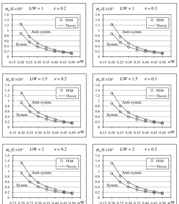
In this section, in order to demonstrate the accuracy and ability of the presented analytical model to estimate the buckling load of the cracked plates with different geometric and material properties, fairly complete comparison between analytical model (Theory) and FEM results are depicted graph-ically in Figures 8 to 10.
Curves depicted in Figure 8 show that with increasing the crack length, buckling capacity of the plates will drop drastically. The reason is that with increasing the crack length, on the one hand, the coefficient β′ increases and on the other hand, the geometric stiffness of the plate decreases and both
factors are simultaneously reducing the buckling capacity of the plate. It is necessary to note that this drop in the anti-symmetric mode is greater than the symmetric mode, so that with increasing crack length, the difference of the two modes decreases but never reaches zero. Therefore, the buckling load in the symmetric mode is often less than the anti-symmetric mode and the symmetric mode can be introduced as the first and prior mode. In contrast, with decreasing the crack length, the buckling load is rising with a steep gradient and it is expected that it tends to infinity at a W =0 because the plates without crack never buckle under tensile load.
Overall, the results of the presented analytical model for different values of crack length have an acceptable agreement with the FEM results in terms of quality and quantity which indicate that the simplifying assumptions of the analytical model are reasonable and do not affect the accuracy. The curves plotted in Figure 9 show that increasing the ratio L W or, in other words, increasing the length of the plate will always increase the buckling capacity. But, the sensitivity of the buckling load to the plate length is reduced by increasing the ratio L W, so that, it looks for L W >2, the buckling load is almost constant.
By comparing Figure 9 with Figure 8, it can be concluded that the buckling load is less sensible to L W than to a W, however, the analytical model is able to show that slight variations of buckling load as well and is in good agreement with the FEM results.
Latin American Journal of Solids and Structures 12 (2015) 2078-2093
Figure 8: Normalized buckling stresses versus relative crack length for both symmetric and anti-symmetric buckling modes.
Moreover, in the Figure 11, the presented approach is compared with some existing experimental works on the symmetric buckling mode, which will be described. The first experimental data was reported by Air Force Flight Dynamics Laboratory (AFFDL) in AFFDL-TR-65-146 (1965) as load versus buckling deflection curves and in the present paper, the extended Southwell technique from NACA TN-658 (1938) is used to estimate the buckling loads from those curves. In the work of Dixon and Strannigan (1969), the upper and lower limits of buckling load are given and here the upper
0 0.2 0.4 0.6 0.8 1 1.2 1.4 1.6
0.15 0.20 0.25 0.30 0.35 0.40 0.45 0.50 0.55a/W FEM Theory
Symm.
Anti-symm.
σcr /E ×103 L/W =1 ν=0.2
0 0.2 0.4 0.6 0.8 1 1.2 1.4 1.6
0.15 0.20 0.25 0.30 0.35 0.40 0.45 0.50 0.55a/W FEM Theory
Symm.
Anti-symm.
σcr /E ×103 L/W =1 ν=0.3
0 0.2 0.4 0.6 0.8 1 1.2 1.4 1.6
0.15 0.20 0.25 0.30 0.35 0.40 0.45 0.50 0.55a/W FEM Theory
Symm.
Anti-symm.
σcr /E ×103 L/W =1.5 ν=0.2
0 0.2 0.4 0.6 0.8 1 1.2 1.4 1.6
0.15 0.20 0.25 0.30 0.35 0.40 0.45 0.50 0.55a/W FEM Theory
Symm.
Anti-symm.
σcr /E ×103 L/W =1.5 ν=0.3
0 0.2 0.4 0.6 0.8 1 1.2 1.4 1.6
0.15 0.20 0.25 0.30 0.35 0.40 0.45 0.50 0.55a/W FEM Theory
Symm.
Anti-symm.
σcr /E ×103 L/W =2 ν=0.2
0 0.2 0.4 0.6 0.8 1 1.2 1.4 1.6
0.15 0.20 0.25 0.30 0.35 0.40 0.45 0.50 0.55a/W FEM Theory
Symm.
Anti-symm.
Latin American Journal of Solids and Structures 12 (2015) 2078-2093
Figure 9: Normalized buckling stresses versus relative plate's length for both symmetric and anti-symmetric buckling modes.
limit is considered. The other experiment was done by Zielsdorff and Carlson (1972) in which the buckling loads were presented and used directly in this paper. The characteristics of these samples are listed in Table 4 and ν = 0.33 is considered for all samples.
From Figure 11, it can be seen that the results of AFFDL-TR-65-146 (1965), with a small distance, are at the top and bottom of the present theoretical curve, so that the theoretical results are well consistent with the mean of the experimental results. Dixon and Strannigan (1969) experiments in-clude a wide range of relative crack lengths and are in very good agreement with the theoretical curve. In the work of Zielsdorff and Carlson (1972), a fewer range of cracks were considered and the difference between the experimental results and the theory increases with decreasing the relative crack length. Looking at three experimental works we can see that for the small cracks, the experimental results show lower values than the analytical results or in other words, the analytical results are somewhat overestimated for small cracks. In sum, given that the experiments were carried out under different conditions and on different materials, Figure 11, can confirm the accuracy of the analytical model based on the experimental results.
0 0.2 0.4 0.6 0.8 1
1.00 1.25 1.50 1.75 L/W+2.00 0.2
0.3 0.4 0.5
σcr /E×103 ν= 0.2
FEM (a/W) Theory
Symm.
0 0.2 0.4 0.6 0.8 1 1.2 1.4
1.00 1.25 1.50 1.75 L/W+2.00 0.2
0.3 0.4 0.5
σcr /E×103 ν= 0.2
FEM (a/W) Theory
Anti-symm.
0 0.2 0.4 0.6 0.8 1
1.00 1.25 1.50 1.75 L/W+2.00 0.2
0.3 0.4 0.5
σcr /E×103 ν= 0.3
FEM (a/W) Theory
Symm.
0 0.2 0.4 0.6 0.8 1 1.2 1.4
1.00 1.25 1.50 1.75 L/W+2.00 0.2
0.3 0.4 0.5
σcr /E×103 ν= 0.3
FEM (a/W) Theory
Latin American Journal of Solids and Structures 12 (2015) 2078-2093
Figure 10: Normalized buckling stresses versus Poisson's ratio for both symmetric and anti-symmetric buckling modes.
Figure 11: Comparison of the presented theoretical model with the experimental data.
0 0.2 0.4 0.6 0.8 1
0.00 0.10 0.20 0.30 0.40 0.50ν+ 0.2
0.3 0.4 0.5
σcr /E×103 L/W= 1
FEM (a/W) Theory
Symm. 0 0.2 0.4 0.6 0.8 1 1.2 1.4 1.6
0.00 0.10 0.20 0.30 0.40 0.50ν+ 0.2
0.3 0.4 0.5
σcr /E×103 L/W= 1
FEM (a/W) Theory
Anti-symm. 0 0.2 0.4 0.6 0.8 1
0.00 0.10 0.20 0.30 0.40 0.50ν+ 0.2
0.3 0.4 0.5
σcr /E×103 L/W= 2
FEM (a/W) Theory
Symm. 0 0.2 0.4 0.6 0.8 1 1.2 1.4 1.6
0.00 0.10 0.20 0.30 0.40 0.50ν+ 0.2
0.3 0.4 0.5
σcr /E×103 L/W= 2
FEM (a/W) Theory
Anti-symm. 0.0 0.5 1.0 1.5 2.0 2.5
0.05 0.10 0.15 0.20 0.25a/L
Theory
AFFDL-TR-65-146 (1965)
Symmetric Mode
σcr /E ×103
0.0 0.5 1.0 1.5 2.0 2.5 3.0
0.1 0.2 0.3 0.4 0.5 0.6 0.7 0.8 0.9 a/W1
Theory
Dixon & Strannigan (1969)
Latin American Journal of Solids and Structures 12 (2015) 2078-2093 Reference Material E (GPa) t (mm) L (mm) W (mm) a(mm)
AFFDL-TR-65-146 (1965) Al2024-T3,T81 70,71 1.52 495 114~305 W 3 Dixon & Strannigan (1969) Al-alloy 68.9 0.94 381 127 19~114 Zielsdorff & Carlson (1972) Al2024-T3 73 0.51 254 152 25.4~30.5
Table 4: Characteristics of experimental samples.
5 CONCLUSIONS
In this paper, an approximate classical solution based on the principle of minimum total potential energy was provided for non-classical local buckling problem of central cracked plate under tension which includes both symmetric and anti-symmetric modes. Given that the mathematical functions for symmetric and anti-symmetric shape modes are written using only 2 and 1 degrees of freedom, the proposed approach mathematically is efficient and has an advantage in comparison with the numerical methods with many degrees of freedom.
After investigating the pre-buckling state, the relative zero point of normal stress σx acting on
the Y -axis (perpendicular to the center of the crack as Figure 3) was defined. Then using the finite element models, it was shown that this point is approximately constant and independent of the plate dimensions so that its theoretical value for the infinite cracked plate can be used for the cracked plates with any sizes. Moreover, the factor β′ was defined as correction factor for the peak
compres-sive stress in the finite cracked plates; then, in order to mathematically describe β′, an empirical
formula was presented based on the finite element results. This correction factor was used in the analytical solution of buckling.
To verify the results of the presented analytical model, a wide range of numerical finite element models (FEM) were produced in ABAQUS environment which can evaluate the effects of the geo-metric characteristics and material properties of the plates on the buckling load. By comparing the results of these models with the results of the analytical model, the accuracy and the ability of the presented analytical model was demonstrated.
Finally, the results of three existing experimental works compared with the presented analytical model that confirm the validity of the analytical model to estimate the buckling load.
References
AFFDL-TR-65-146 (AFFDL), (1965). Technical Report – Experimental program to determine effect of buckling and specimen dimensions on fracture toughness of thin sheet materials.
Brighenti, R., (2005a). Numerical buckling analysis of compressed or tensioned cracked thin plates. Engineering struc-tures 27: 265–276.
Brighenti, R., (2005b). Buckling of cracked thin-plates under tension or compression. Thin-Walled Structures 43: 209– 224.
Brighenti, R., (2009). Buckling sensitivity analysis of cracked thin plates under membrane tension or compression loading. Nuclear Engineering and Design 239: 965–980.
Cherepanov, G.P., (1963). On the buckling under tension of a membrane containing holes. Applied Mathematics and Mechanics 27(2): 275-286.
Latin American Journal of Solids and Structures 12 (2015) 2078-2093
Dyshel, M.S., (1990). Stress-intensity coefficient taking account of local buckling of plates with cracks. International Applied Mechanics 26: 98-103.
Dyshel, M.S., (1999). Local buckling of extended plates containing cracks and cracklike defects, subject to the influence of geometrical parameters of the plates and the defects. International Applied Mechanics 35: 1272-1276.
Dyshel, M.S., (2002). Stability and fracture of plates with a central and an edge crack under tension. International Applied Mechanics 38: 472-476.
Guz, A.N., Dyshel, M.Sh., Nazarenko, V.M., (2004). Fracture and stability of materials and structural members with cracks approaches and results. International Applied Mechanics 40: 1323-1359.
Isida, M., (1971). Effect of width and length on stress intensity factors of internally cracked plates under various boundary conditions. International Journal of Fracture Mechanics 7: 301-316.
Markstrom, K., Storakers, B., (1980). Buckling of cracked members under tension. International Journal of Solids and Structures 16: 217–229.
Riks, E., Rankin, C.C., Brogan, F.A., (1992). The buckling behavior of a central crack in a plate under tension. Engineering Fracture Mechanics 43: 529–548.
Sadd, M.H., (2005). Elasticity: Theory, Applications and Numerics. Elsevier Inc, Oxford.
Shaw, D., Huang, Y.H., (1990). Buckling behavior of a central cracked thin plate under tension. Engineering Fracture Mechanics 35: 1019-1027.
Sih, G.C., Lee, Y.D., (1986). Tensile and compressive buckling of plates weakened by cracks. Theory and Applied Fracture Mechanics 6: 129–138.
TN-658 (NACA), (1938). Technical Notes – Generalized analysis of experimental observations in problems of elastic stability.