Lat. Am. j. solids struct. vol.12 número11

(1)

Abstract

The widespread use of tubular sections in regions like Western Europe and North America in addition struc-tural and aesthetical reasons can be attributed to the high degree of development of their production technol-ogy. Despite this fact their use in Brazil in the past was limited to a few spatial roofs. Currently, the situation in the Brazilian market begins to change caused by the significant increase in the availability of structural hol-low sections. This work presents an analysis of “KK” joints with circular hollow sections. A comparison be-tween the analytical design formulations proposed by the Eurocode 3 Part 1.8, the 2nd edition of the CIDECT tubular joint design guide was performed.A finite ele-ment model was developed in the ANSYS program for each analysed joint typology.The modelling of a spatial truss made of circular hollow section elements was also performed to enable a comparison between a single joint and the response of the joint as a part of a full scale truss structure.

Keywords

Tubular sections; finite element model; spatial truss.

Evaluation of CHS tubular KK joints

1 INTRODUCTION

The widespread use of tubular sections in regions like Western Europe and North America can be attributed to the high degree of development of their production technology. Despite this fact their use in Brazil in the past was limited to a few spatial roofs. Currently, the situation in the Brazilian market begins to change caused by the significant increase in the availability of structural hollow sections. In addition, their associated aesthetical and structural advantages led designers to focus on the technologic and design issues and contributed to their worldwide use (an example is illustrated in Figure 1).

David Silva Nobrea

Luciano R.O. de Limab

Pedro C.G. da S. Vellascoc Luis F. Costa-Nevesd André T. da Silvae

a_{PGECIV. Civil Engineering Post-Graduate}

Pro-gram. UERJ – State University of Rio de Janeiro. Brazil

b,c,e_{Structural Engineering Department. UERJ –}

State University of Rio de Janeiro. Brazil

d_{INESCC. Civil Engineering Department – FCTUC –}

University of Coimbra. Portugal

Corresponding author:

a_{david_nobre17@yahoo.com.br} b_{lucianolima@uerj.br}

c_{vellasco@eng.uerj.br} d_{luis@dec.uc.pt} e_{tenchini@eng.uerj.br}

http://dx.doi.org/10.1590/1679-78251789

(2)

Latin American Journal of Solids and Structures 12 (2015) 2143-2158

Design methods accuracy is a key instrument to achieve an economical and safe design, and recent tubular joint studies indicate that further research is needed, especially for some particular geometries characterized by failure modes with corresponding load predictions that are unsafe or uneconomical. One of the first comprehensive investigation in this area was published by Korol and Mirza (1982) that developed a numerical model with shell elements. These authors concluded for simultaneous increase of the joint resistance and the variable β and/or the decrease of the variable γ. These

authors also indicated the need of establishing a deformation limit criterion for these connections. Recently, Lu et al.(1994), cited by Kosteski et al. (2003), with results also validated and accepted by Zhao (2000) established an approximate 3% d₀ (chord diameter) deformation limit for the loaded

section face corresponding to the joint ultimate limit state. This 3% d₀ limit (N_u) is currently widely

accepted and is the limit adopted by the International Institute of Welding (IIW) for the maximum acceptable displacement associated to the ultimate limit state, while a 1% d₀ limit (N_s) is adopted

for the serviceability limit state establishment. If the ratio N_u N_s is greater than 1.5, the joint

strength should be based on the serviceability limit state. Alternatively if N_u N_s < 1.5 the ultimate

limit state controls the design and the 3% d₀ limit (N_u) applies. In the case of CHS joints, most

frequently N_u N_s> 1.5, and therefore the appropriate deformation limit to establish the ultimate

joint strength should be 0.03d0.

Figure 1: Example of a structure with hollow sections.

This paper presents a numerical model (i.e. nonlinear FEM simulations) used to perform a parametric study dealing with the behavior of CHS (circular hollow sections) tubular KK joints. The proposed model was validated by comparisons to experiments (Lee and Wilmshurst, 1997), to design standard predictions like Eurocode 3 (2003), ABNT NBR16239 (2013) and the new CIDECT (Wardenier et al., 2008) and finally to classic deformation limits present in literature. The main variables of the present study were the brace diameter to chord diameter ratio and the chord face diameter to chord thickness ratio. These parameters were chosen based on recent studies that indicated some discrep-ancies between Eurocode 3 (2003) rules and numerical results.

(3)

Latin American Journal of Solids and Structures 12 (2015) 2143-2158 loading of the braces. Multiple regression analysis was performed to obtain prediction equations. The proposed ultimate strength equations are shown to be in agreement with the test results. The predic-tion models were based on a simple mechanical model of a ring that enables an extrapolapredic-tion of the geometric variables' application ranges. The proposed ultimate strength equations were compared to existing prediction formulas. For the proposed validity ranges of the ultimate strength equations, the multi planar coefficient µ, the factor by which the uniplanar joint strength has to be multiplied to

obtain the multi planar joint strength, ranged from 0.5 to 1.3, indicating that multi planar effects were insignificant, as stated by Paul et al. (1994).

A numerical study on the static strength of CHS (circular hollow section) joints with the multi planar double-K configuration was presented by Lee and Wilmshurst (1997). The aim of the work was to establish a valid and accurate finite element model for an extensive parametric study aiming to investigate the various factors which influence the static strength. These factors included modelling the effect of the weld geometry, boundary conditions at chord and brace ends, mode of loading, chord length and material properties. The numerical results were rigorously calibrated against existing ex-perimental data. The study provided an insight into the many aspects of elastic-plastic finite element analysis which is gradually replacing experimental tests as the main tool of research in tubular joint technology.

Mendes (2008) performed a study with theoretical, numerical and experimental approaches of welded K-, KT- and T-joints of HSS profiles, using RHS in the chord and CHS in the other structural elements. An analytical study was performed, using code recommendations (Eurocode 3 - Part 8, 2005), and some comparisons were established with the numerical and experimental results. This author found a good agreement for these sets of results for T-joints, but the results for K- and KT-joints showed the need for further improvement.

Gazzola et al. (2000) assessed the axial load effect in tubular welded K-joints using finite element techniques and compared the results to available analytical formulations, concluding that additional researches should be performed for this joint type. Lee and Gazzola (2006) investigated numerically the overlap effect for K-joints under bending moment.

Forti (2010) performed a parametric study investigating the behavior of K- and KK-joint using circular hollow sections with spacing between diagonals and being symmetrically loaded. The joints types’ behavior was compared using a numerical model developed in ANSYS (2010). Two additional parametrical studies were made with 55 KK-joints and similar K-joints. From these studies, the dominant failure KK-joints modes based in diametric deformation could be established, and their relevance as a function of the spacing between diagonals.

Silva (2012) investigated the behavior of K- and T-joints with circular hollow sections and estab-lished comparisons between the analytical formulations proposed by Eurocode 3 – Part 8 (2005), the 2nd edition design guide of tubular joints of the Wardenier et al. (2008), the Brazilian code – NBR 16239:2013 (2013) and the deformation limit criteria (Lu et al., 1994). For each of the analyzed joint types, a finite element model was developed in ANSYS (2010) being calibrated and validated with experimental and numerical results present in the literature. The material and geometric nonlineari-ties were incorporated into the models to fully mobilize the resistance capacity of the joint. Analysis of models with and without chord loading enabled this author to conclude that the ratio between the loads associated with the ultimate and service limit states remains smaller than 1.50, in other words,

1.50

u s

(4)

2 EUROCODE 3 AND CIDECT DESIGN PROVISIONS

According to Eurocode 3 (2003); ABNT NBR16239 (2013); Wardenier et al. (2008), some geometrical limits need to be verified prior to the evaluation of the joint resistance. These limits are presented in Figure 2 where d₀, d_i, t₀, t_i, θ, φ, g_l, g_t and L represent respectively, the chord diameter, the

brace diameter, the chord thickness, the brace thickness, the angle between chord axis and plane in which compression braces lie, the out-of-plane angle between the planes in which the braces lie, the longitudinal gap between braces, the transverse gap between braces and the chord length. When CHS KK-joints are considered, some ultimate limit states should be verified. Despite this fact, chord yield-ing controlled the CHS KK joint design in all considered cases. Eurocode 3 (2003) and ABNT NBR16239 (2013) expresses this ultimate limit state in equation (7) based on CHS KK joint with a reduction factor of 0.9.

30º≤θi ≤90º (1)

1

0

0.2 d 1

d

β

≤ = ≤ (2)

0 0

0

10 d 50

t

µ

≤ = ≤ (3)

10 i 50

i i

d t

µ

≤ = ≤ (4)

0

2

d t

γ = (5)

1 2

g ≥t +t (6)

(

)

2

1,Rd 0.9 g p y0 0 1.8 10.2 1 0 M5 sin

N = k k f t + ×d d γ θ (7)

(

)

0.2 1.2

0

1 0.024 exp 0.5 1.33 g

k = γ __ + γ g t − __ (8)

Where N_1,_Rd is the chord face failure resistance;

γ is a geometrical parameter according to equation (5);

p

k is taken equal to 1.0;

g

k is a parameter according to equation (8);

0 y

f is the chord yield stress taken equal to 355 MPa in parametrical analysis;

β is a geometrical parameter according to equation (2);

5 M

γ is the partial safety factor, in this case, equal to 1.

The joint strength Eq. (9) for chord yielding limit state according to Wardenier et al. (2008) is expressed in terms of Qu (influence of the parameters β and γ) and Qf (influence of the parameter

n). In these equations, the parameter C₁ is taken as 0.25 for chord compression stresses (n <0) and

(5)

(a) (b)

(c)

Figure 2: Geometrical limits of a KK tubular joint.

2 0 0 *

1

sin

y

i u f

f t N Q Q

θ

= with 0,3

₍

1,6

₎

0.8

0

1.65 1 8 1 1 1.2 ( )

u

Q = γ + β __ + + g t __ (9)

0 0

,0 ,0

pl pl

N M

n

N M

= +

(

)

1

1 C

f

Q = − n (10)

3 NUMERICAL MODEL

The proposed numerical model adopted shell elements available in the ANSYS Element Library (AN-SYS, 2010). The model was developed using four-node thick shell elements (SHELL181), therefore considering bending, shear and membrane deformations. The finite element mesh was more refined near the welds, where the stress concentration is more likely to occur, and as more regular as possible, with well-proportioned elements to avoid numerical problems. The welds were modelled with shell elements according to Lee (1999), see Figure 3, presenting an overview of the developed finite element model. Loading was applied by displacing the nodes at the left end of the chord while the right end was left unrestrained. This simulated the test set-up described by Lee (1999) that was used to cali-brate the numerical model. A full nonlinear analysis was performed considering material and geomet-rical nonlinearities.

L

0

/2

d

0

t

0

t

1

L

0

/2

d

0

d

1

t

1

d

1

L

0

/2

L

0

/2

d

0

t

1

(6)

a) full model b) weld detail c) weld model after Lee (1999)

Figure 3: CHS KK joint model.

A parametric study varying some geometrical parameters was performed to evaluate their influence in the connection resistance. The adopted material constitutive law presented a bilinear behaviour with a slight strain-hardening before failure with a yield stresses of 355 MPa and 600 MPa for con-nected members and weld elements, respectively. Table 1 presents the variables used in the parametric study, in which 19 simulations were performed. It is important to emphasise that the corresponding parameters combinations were chosen considering the limits imposed by the chord bending moment and brace normal plastic resistances. A single section for the chord was used, 114.3x4.4 mm, with four different brace diameters. 38, 44.5, 46 and 50.8 mm, all with a 3 mm thickness. The weld thickness was adopted as the minimum thickness of the plates to be connected. In this table the joint resistance considering the chord yielding failure according to Eurocode 3 (2003) and Wardenier et al. (2008) are also presented. It is important to mention that, for all studied cases, the CIDECT resistance values were greater than those obtained from the Eurocode 3 (2003) provisions.

4 NUMERICAL RESULTS

As previously explained for this joint type, the ultimate limit state that governs the joint design is the chord yielding. According to the deformation limit criterion of 3% d₀ (see Lu et al., 1994; Zhao

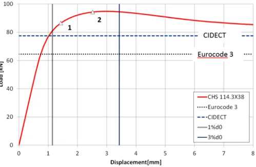
2000), for the studied joints, the chord out of plane displacement limit is 3.43 mm. Aiming at identi-fying and confirming the initial assumptions regarding the ultimate limit state for CHS tubular joints, the von Mises stress distribution for a joint between a 114.3x4.4 mm chord and a 38.0x3 mm brace was analyzed and the results are presented in Figure 4. It may be observed that the joint failure is controlled by the chord yielding and that the Eurocode 3 and CIDECT resistances are less than the joint ultimate load. If the partial coefficient factor γM₅ is used, the joint design will lead to even more conservative limits. The application of the deformation limit criterion (Nu and Ns) is summarized in Table 1, Table 2, Table 3 and Table 4. The load-displacement curve for the joint 114.3x38 is plotted in Figure 5 with the application of the 3% d₀ criterion, and where two levels of force are

highlighted, point (1) in the elastic range and point (2) corresponding to the von Mises stresses, according to Figure 4 (a) and (b), respectively.

(7)

Latin American Journal of Solids and Structures 12 (2015) 2143-2158 a) applied load = 86.5 kN (point 1) a) applied load = 94.3 kN (point 2)

Figure 4: CHS 114.3x4.4 with 38x3 – Von Mises stress distribution.

Figure 5: Load-displacement curve: deformation limit criterion application.

5 GLOBAL TRUSS

5.1 Truss Structures analysis

(8)

REF d₁ θ φ g_l g_t β N_s N_u N_peak N_1,Rd N₁∗ [1]

1,Rd

N N *

1 N N

KK-01 38.0 60o 90o 35.0 49.5 0.33 80.86 94.45 94.79 64.05 77.47 0.68 0.82 KK-02-A 38.0 60o 45o 55.0 49.5 0.33 75.33 89.61 62.15 74.75 0.69 0.83 KK-02-B 38.0 60o 45o 35.0 49.5 0.33 73.70 87.36 64.05 77.47 0.73 0.89 KK-03 38.0 60o 60o 35.0 21.2 0.33 83.37 97.42 64.05 77.47 0.66 0.80 KK-04 38.0 60o 60o 55.0 21.2 0.33 78.95 95.50 62.15 74.75 0.65 0.78 KK-05 38.0 60o 75o 35.0 35.5 0.33 84.42 96.72 97.21 64.05 77.47 0.66 0.80 KK-06 38.0 60o 75o 55.0 35.5 0.33 76.39 94.14 62.15 74.75 0.66 0.79 KK-07 44.5 60o ₉₀o _35.0 _43.1 _0.39 _91.63 _108.36 _71.21 _90.36 _0.66 _0.83

KK-08-A 44.5 60o 45o 55.0 43.1 0.39 83.82 97.55 69.10 87.18 0.71 0.89 KK-08-B 44.5 60o 45o 35.0 43.1 0.39 82.15 93.34 71.21 90.36 0.76 0.97 KK-09 44.5 60o ₆₀o _35.0 _14.3 _0.39 _93.26 _107.82 _71.21 _90.36 _0.66 _0.84

KK-10 44.5 60o 60o 55.0 14.3 0.39 88.59 105.61 69.10 87.18 0.65 0.83 KK-11 44.5 60o 75o 35.0 28.8 0.39 94.85 110.00 71.21 90.36 0.65 0.82 KK-12-A 44.5 60o ₅₀o _55.0 _28.8 _0.39 _86.89 _101.97 _69.10 _87.18 _0.68 _0.85

KK-12-B 44.5 60o 50o 35.0 28.8 0.39 86.28 98.40 71.21 90.36 0.72 0.92 KK-13-A 46.0 60o 45o 35.0 41.3 0.40 84.12 95.18 72.86 93.50 0.77 0.98 KK-13-B 46.0 60o ₄₅o _55.0 _41.3 _0.40 _85.84 _99.36 _70.70 _90.22 _0.71 _0.91

KK-17 50.8 60o 60o 35.0 7.4 0.44 102.48 117.16 78.14 103.97 0.67 0.89 KK-19 50.8 60o 75o 35.0 22.0 0.44 104.98 121.28 78.14 103.97 0.64 0.86

[1]_If

u s

N N <1.5 then N =Nu else N =Ns.

If there is a Npeak, its value controls the design.

Dimensions in mm and loads in kN.

Table 1: Summary of first group of the numerical models (d₀ =114.3, t₀=4.4, σ_y =355 MPa and t₁=3).

REF d₁ θ φ g_l g_t β=d d₁ ₀ N_peak N_1,Rd N₁∗ [1] 1,Rd

N N *

1 N N

P-KK-21 38.0 60o 90o 35 69.5 0.27 84.93 59.05 68.81 0.70 0.81 P-KK-22 38.0 60o ₉₀o ₅₅ _69.5 _0.27 _81.62 _56.81 _66.39 _0.70 _0.81

P-KK-23 38.0 60o 60o 35 35.4 0.27 91.00 59.05 68.81 0.65 0.76 P-KK-24 38.0 60o 60o 55 35.4 0.27 87.17 56.81 66.39 0.65 0.76 P-KK-25 38.0 60o ₇₅o ₃₅ _52.7 _0.27 _89.10 _59.05 _68.81 _0.66 _0.77

P-KK-29 44.5 60o 90o 35 63.5 0.31 94.55 65.15 78.59 0.69 0.83 P-KK-30 44.5 60o 90o 55 63.5 0.31 92.86 62.68 75.83 0.67 0.82 P-KK-31 44.5 60o ₆₀o ₃₅ _28.8 _0.31 _101.27 _65.15 _78.59 _0.64 _0.78

P-KK-32 44.5 60o 60o 55 28.8 0.31 97.07 62.68 75.83 0.65 0.78 P-KK-33 44.5 60o 75o 35 46.3 0.31 99.21 65.15 78.59 0.66 0.79 P-KK-34 44.5 60o ₇₅o ₅₅ _46.3 _0.31 _93.09 _62.68 _75.83 _0.67 _0.81

P-KK-35 44.5 60o 85o 55 57.8 0.31 92.51 62.68 75.83 0.68 0.82 P-KK-36 50.8 60o 90o 35 57.4 0.36 105.27 71.06 88.93 0.68 0.84 P-KK-37 50.8 60o ₉₀o ₅₅ _57.4 _0.36 _105.12 _68.37 _85.81 _0.65 _0.82

P-KK-41 50.8 60o 75o 55 39.7 0.36 103.84 68.37 85.81 0.66 0.83 P-KK-42 50.8 60o 80o 55 51.6 0.36 103.84 68.37 85.81 0.66 0.83

[1]_If

u s

Dimensions in mm and loads in kN

(9)

Latin American Journal of Solids and Structures 12 (2015) 2143-2158 REF d₁ g_t g_l β=d d1 0 Ns Nu Npeak N1,Rd N1∗

[1] 1,Rd

N N *

1 N N

SKK-02 28.8 33.4 28 0.24 91.64 82.65 97.19 72.97 80.38 0.75 0.83 SKK-03 28.8 33.4 38 0.24 92.31 89.42 100.71 69.51 78.09 0.69 0.78 SKK-04 28.8 33.4 48 0.24 92.98 104.65 68.00 76.56 0.65 0.73 SKK-05 28.8 33.4 58 0.24 92.00 103.36 67.40 75.45 0.65 0.73 SKK-06 28.8 33.4 68 0.24 89.88 100.28 101.88 67.17 74.61 0.67 0.74 SKK-08 38.4 23.6 28 0.32 111.50 118.36 121.16 86.99 101.48 0.73 0.86 SKK-09 38.4 23.6 38 0.32 109.93 122.34 82.87 98.60 0.68 0.81 SKK-10 38.4 23.6 48 0.32 111.03 124.26 81.06 96.66 0.65 0.78 SKK-11 38.4 23.6 58 0.32 111.26 125.47 80.35 95.27 0.64 0.76 SKK-13 48.0 13.4 28 0.40 128.57 142.06 101.01 126.03 0.71 0.89 SKK-14 48.0 13.4 38 0.40 126.48 138.18 96.22 122.45 0.70 0.89 SKK-15 48.0 13.4 48 0.40 125.78 139.22 94.12 120.05 0.68 0.86

[1]_If

u s

Table 3: Summary of the third group of the numerical models (d₀=120 mm, θ =56,3o_,_φ ₌₆₀o _and

y

σ =355 N/mm²).

REF d₁ g_t g_l β =d d₁ ₀ N_s N_u N_peak N_1,Rd N₁∗ N1,Rd N[1] * 1 N N

SKK-03-B 28.8 33.4 38 0.24 42.55 38.77 43.36 24.64 28.91 0.57 0.67 SKK-03-C 28.8 33.4 38 0.24 22.87 17.28 23.00 12.89 15.39 0.56 0.67 SKK-03-D 28.8 33.4 38 0.24 12.67 9.38 13.25 7.68 9.30 0.58 0.70 SKK-09-A 38.4 23.6 38 0.32 177.43 201.59 - 142.33 165.35 0.71 0.82 SKK-09-B 38.4 23.6 38 0.32 53.90 51.28 54.55 29.37 36.50 0.54 0.67 SKK-09-C 38.4 23.6 38 0.32 28.77 21.04 28.95 15.36 19.43 0.53 0.67 SKK-09-D 38.4 23.6 38 0.32 16.18 11.46 17.17 9.15 11.74 0.53 0.68 SKK-09-H 38.4 23.6 38 0.32 119.89 129.39 - 82.87 98.60 0.64 0.76 SKK-09-I 38.4 23.6 38 0.32 75.37 83.12 83.46 54.53 66.20 0.66 0.80 SKK-09-J 38.4 23.6 38 0.32 47.42 44.72 49.53 29.37 36.50 0.59 0.74 SKK-14-A 48.0 13.4 38 0.40 202.97 225.82 - 165.27 205.35 0.73 0.91 SKK-14-B 48.0 13.4 38 0.40 60.22 58.62 61.42 34.10 45.33 0.56 0.74 SKK-14-C 48.0 13.4 38 0.40 35.00 25.92 35.14 17.84 24.13 0.51 0.69 SKK-14-D 48.0 13.4 38 0.40 20.12 14.04 21.54 10.63 14.58 0.49 0.68

[1]_If

u s

Table 4: Summary of the fourth group of the numerical models (d₀ =120 mm, θ=56,3o, φ=60o and σ_y =355 N/mm²).

(10)

Latin American Journal of Solids and Structures 12 (2015) 2143-2158 5.2 Model with eccentricity – Shell Elements – Nonlinear Analysis

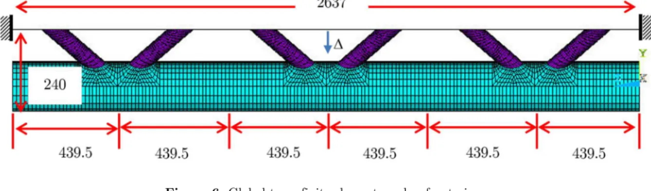
Aiming to investigate the applicability of the design equations for welded KK-joints using hollow sections, as well as to compare the behavior of the isolated joint with the behavior of the same joint integrated in a conventional truss system, a numerical model for a spatial truss with three KK-joints was developed, as illustrated in Figure 6. The boundary conditions – fully rigid supports at the upper extremities – as well as the point of application of the prescribed displacement at mid-span may be depicted.

Full nonlinear analyses considering geometric and material nonlinearities were performed, aiming to reproduce the behavior of a real truss structure. It should be referred that the original truss di-mensions were changed (flange and diagonal thicknesses enhanced to 8 mm and to 6 mm respectively) to force the joints to control the design, as depicted in Table 5.

A 40 mm thick plate was used in the upper part of the spatial truss modelled with SHELL181 elements and a linear elastic material, having the sole objective of transmitting the load applied to the KK-joint diagonals.

Figure 6: Global truss finite element mesh – front view.

Joint d₀

[mm]

0

t

[mm]

1

d

[mm]

1

t

[mm]

1 0

d d

β = γ =d₀ 2t₀ τ =t t₁ ₀ θ

DKA1-M 217 8 77.7 6 0.36 13.37 0.75 60o

Table 5: Geometrical properties – global truss.

(11)

Latin American Journal of Solids and Structures 12 (2015) 2143-2158 Figure 7: Global truss finite element mesh – isometric view.

Figure 8: Weld region detail.

5.3 KK-Joint between circular hollow sections – Isolated joint versus joint integrated in a truss

(12)

Figure 9: Load versus Displacement: Trussed node versus Isolated node.

For the isolated joint, the loads corresponding to the serviceability limit state, N_s, was 350.8 kN; for the ultimate limit state, N_u, 331.03 kN; and that for the peak, N_peak, was 357.39 kN at the compres-sion brace. For the tencompres-sion brace, the load for the serviceability limit state, Ns, was 336.55 kN; for the ultimate limit state, N_u, was 366.72 kN; and for the peak, N_peak, was 366.81 kN. In both situations there was a load peak between the 1% and 3% levels indicating that the peak load controlled the joint design.

As far as the truss joint is concerned, and referring to the compression brace, the load for the serviceability limit state, N_s, was 327.29 kN; and for the ultimate limit state, N_u, was 427.69 kN. With respect to the tension brace, the load for the serviceability limit state, N_s, was 333.4 kN and that for the ultimate limit state, N_u, was 454.46 kN.In these two last situations, the ratio N_u N_s

was less than 1.50, i.e., indicating the ultimate limit state load controlled the joint design. Figure 9 also shows that the design load of the connection was 297.8 kN according to the equation proposed by Eurocode 3 (2003) and 334.2 kN according to the Wardenier et al. (2008) recommendations. Comparing the curves for the global truss and for isolated joints a 25% difference may be depicted, that may be caused by differences in the boundary conditions adopted in the two investigated models. In the isolated joint model the chord was considered as simply supported, while in the global truss the joint had more flexible boundaries, since the restrictions were applied to the upper chord. Fur-thermore, the load application method in the two models was different; in the isolated joint the load was directly applied to the diagonals, whereas the load was applied at the truss upper chord center. The difference between the analyses represents a bolder design for the isolated joint when compared to the joint belonging to a conventional truss system. In addition, the equation proposed by Wardenier et al. (2008) shows a good agreement to the limit deformation criterion for both situations, though being more accurate for the isolated joint.

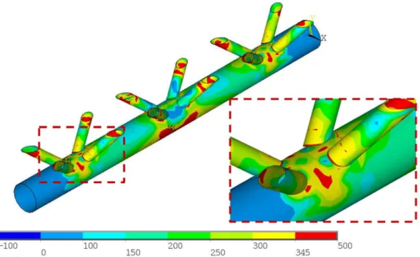
Figure 10 illustrates the points for which the Von Mises stresses depicted in Figure 11, Figure 12 and Figure 13, showing that yielding first occurs in the chord than in the diagonals. In these illustra-tions, only the chord and the diagonals (not the top plate nor the welds) are presented.

0 50 100 150 200 250 300 350 400 450 500

0 2 4 6 8 10 12 14 16 18 20

Lo a d [ k N ] Displacement [mm]

COMPRESSION BRACE -ISOLATED NODE TENSION BRACE - ISOLATED NODE

COMPRESSION BRACE -TRUSSED NODE TENSION BRACE - TRUSSED NODE

EC3 1-8/ NBR 16239:2013

(13)

Latin American Journal of Solids and Structures 12 (2015) 2143-2158 Figure 10: Load displacement curve for the investigated truss.

Figure 11: Von Mises stresses (MPa) Tension brace axial load = 259.9 kN and displacement = 1.43 mm (Point 1).

6 FINAL REMARKS

This paper presented a numerical study of CHS KK tubular joints performed with the finite element package ANSYS (2010). The numerical results were compared to analytical results proposed by Eurocode 3 (2003); Wardenier et al. (2008) recommendations. It is important to emphasise that

0 50 100 150 200 250 300 350 400 450 500

0 2 4 6 8 10 12 14 16 18 20

Lo

a

d

[

k

N

]

Displacement [mm]

Tension Brace 1% 3%

1

2

(14)

Figure 12: Von Mises stresses (MPa) – Tension brace axial load = 343.5 kN and displacement = 2.32 mm (Point 2).

(15)

Latin American Journal of Solids and Structures 12 (2015) 2143-2158 for this joint type, the Eurocode 3 (2003) results were more conservative when compared to their Wardenier et al. (2008) counterparts. The ultimate limit state for this joint type was the chord yielding according to the Eurocode 3 (2003); Wardenier et al. (2008) and to the numerical results. As depicted in Table 1, the numerical resistances obtained from the application of the deformation limit criterion were higher than those obtained from the application of the Eurocode 3 (2003) provi-sions, showing this code safety. The ratio N₁∗ N is closer to 1 than the ratio N_1,_Rd N , as could be

observed in Table 1. This fact indicates that Wardenier et al. (2008) formulation is more accurate than the Eurocode 3 (2003) formulation.

Comparing a joint belonging to a conventional truss system to an isolated joint, there was a difference of approximately 25% that may be considered reasonable in the context of this paper. It is observed that this difference represents a more economical design for the joint within a truss when compared to the isolated joint. It follows also that the proposed design by Wardenier et al. (2008) presents a good agreement with the application of the deformation criterion for both situations, and is more accurate for the isolated joint.

References

ABNT NBR 16239:2013, (2013). Projetos de estrutura de aço e de estruturas mistas de aço e concreto de edificações com perfis tubulares.

ANSYS 12.0 ®, (2010), ANSYS, Inc., Theory Reference.

Eurocode 3, ENV 1993-1-1, (2003). Design of steel structures - Structures – Part 1-1: General rules and rules for buildings. CEN, European Committee for Standardisation, Brussels.

Eurocode 3, EN 1993-1-8, (2005). Design of steel structures - Structures – Part 1-8: Design of joints. CEN, European Committee for Standardisation, Brussels.

Forti, N.C.S., (2010). Estudo paramétrico de estruturas tubulares com ligações multiplanares. PhD thesis, Universidade Estadual de Campinas.

Gazzola, F., Lee, M.M.K., Dexter, E.M., (2000). Design equation for overlap tubular K-joints under axial loading. Journal of Structural Engineering 126(7): 798-808, ASCE.

Korol, R., Mirza, F., (1982). Finite element analysis of RHS T-joints. Journal of the Structural Division 108: 2081-2098, N. ST9, ASCE.

Kosteski, N., Packer, J.A., Puthli, R.S., (2003). A finite element method based yield load determination procedure for hollow structural section connections. Journal of Constructional Steel Research 59: 453-471.

Lee, M.K.K., (1999). Strength, stress and fracture analyses of offshore tubular joints using finite elements. Journal of Constructional Steel Research 51: 265-286.

Lee, M.M.K., Gazzola, F., (2006). Design equation for offshore overlap tubular K-joints under in-plane bending. Journal of Structural Engineering 1329(7): 1087-1095, ASCE.

Lee, M.M.K., Wilmshurst, S.R., (1997). Strength of multiplanar tubular KK-joints under antisymmetrical axial load-ing. Journal of Structural Engineering 123(6): 755.764.

Lima, N.S., (2012). Comportamento estrutural de ligações tubulares T e KT. MSc thesis, Universidade do Estado do Rio de Janeiro, Faculdade de Engenharia, Programa de Pós-Graduação em Engenharia Civil.

(16)

Mendes, F.C., (2008). Análise teórica-experimental de ligações tipo “T”, “K” e “KT” com perfis metálicos tubulares. MSc thesis, Universidade Federal de Ouro Preto.

Paul, J.C., Makino, Y., Kurobane, Y., (1994). Ultimate resistance of unstiffened multiplanar tubular TT and KK-joints. Journal of Structural Engineering 120(10): 2853-2870.

Silva, R.S., (2012). Avaliação de ligações K e T entre perfis estruturais tubulares circulares. MSc thesis, Universidade do Estado do Rio de Janeiro.

Wardenier, J., Kurobane, Y., Packer, J.A., van der Vegte, G.J., Zhao, X.-L., (2008). Design guide for circular hollow section (CHS) joints under predominantly static loading. CIDECT, 2nd. Edition, "Construction with Hollow Steel Sections series", Verlag TUV Rheinland, 2008.