Lat. Am. j. solids struct. vol.12 número11

(1)

Abstract

A transition element is developed for the local global analysis of laminated composite beams. It bridges one part of the domain modelled with a higher order theory and other with a 2D mixed layerwise theory (LWT) used at critical zone of the domain. The use of developed transition element makes the analysis for interlaminar stresses possible with significant accuracy. The mixed 2D model incorporates the transverse normal and shear stresses as nodal degrees of freedom (DOF) which inherently ensures continuity of these stresses. Non critical zones are modelled with higher order equivalent single layer (ESL) theory leading to the global mesh with multiple models applied simultaneously. Use of higher order ESL in non critical zones reduces the total number of elements required to map the domain. A substantial reduction in DOF as compared to a complete 2D mixed model is obvious. This computationally economical multiple modelling scheme using the transition element is applied to static and free vibration analyses of laminated composite beams. Results obtained are in good agreement with benchmarks available in literature.

Keywords

Mixed formulation; finite element method; laminated composite beams; transition element; local global analysis; Hamilton's variational principle; principle of minimum potential energy.

Multi-model finite element scheme for static and free vibration

analyses of composite laminated beams

1 INTRODUCTION

Laminated composites are finding varied engineering applications as these materials possess a good environmental resistance, strength and are light in weight. Failure modes of laminated composites include the delamination failure leading to separation of the layers and loss of integrity of the structure. Due to the heterogeneous material properties of the different layers of the composite laminate high interlaminar stresses develop at the interfaces. For the kinetic equilibrium in the thickness direction, these interlaminar stresses need to be continuous between the layers. Pipes and

U.N. Banda* Y.M. Desaib

a,b_{Department of Civil Engineering,} Indian Institute of Technology Bombay, Powai, Mumbai - 400076, India. b_{JK & MJ Mehta Chair Professor} b_{desai@civil.iitb.ac.in}

Corresponding author: a*_{umeshband@gmail.com}

http://dx.doi.org/10.1590/1679-78251743

(2)

Latin American Journal of Solids and Structures 12 (2015) 2061-2077

Pagano (1970); Rybicki (1971) brought out that delamination failure can be attributed to the interlaminar transverse shear and normal stresses. For a sound design, an accurate evaluation of the interlaminar stresses becomes inevitable. Different analytical and finite element equivalent single layer (ESL) and layerwise (LW) models have been proposed for analysis of composites. The ESL models in the literature predict the global parameters with a reasonable accuracy but fail to predict the continuity of interlaminar stresses. The displacement based LW models also fail to predict continuity of transverse stresses. These are more accurate relative to ESL models for global parameters but need higher computational effort. For estimation of the transverse stresses, a separate stress function or integration of stress equilibrium equations is essential. LW mixed model with transverse stresses as nodal DOF are accurate for global parameters and also for local interlaminar stresses.

Accurate elastic analysis of interlaminar stresses in composite laminates was presented by Srinivas and Rao (1970); Pagano (1969, 1970); Pagano and Hatfield (1972). As an offshoot of the plate formulation, many researchers have presented theories for analysis of composite laminated beams. Kant (1982) presented a comprehensive higher order theory for analysis of thick plates. Kant et al. (1997) applied the fully cubic theory for the dynamic analysis of beams. Various forms of higher order sub-theories were evolved by eliminating some terms from the comprehensive cubic theory (Marur and Kant, 1996; Manjunatha and Kant, 1993a; 1993b). Reddy (1987) presented higher order ESL as well as displacement based LW formulations. Contributions were also made by Lo et al. (1978); Spilker (1982), and others in the form of higher order theories. The formulation of Spilker had a stress based hybrid element having separate through thickness distributions for stress and displacements. To overcome the limitation of displacement based ESL, Rao et al. (2001) proposed an analytical solution based on mixed formulation in which the transverse stresses are invoked as DOF ensuring their continuity. This model has been employed for static and dynamic analyses of laminated plates and beams. Shimpi and Ghugal (1999) presented a trigonometric shear deformable LW theory capable of maintaining the continuity of transverse stresses. Desai and Ramtekkar (2002) presented a mixed finite element LW model with transverse stresses also included in the set of nodal DOF. The issue of continuity is inherently resolved and the results are seen to be in good agreement with the exact solutions. The formulation was applied to static analysis of composite beams. Ramtekkar et al. (2002) extended the mixed formulation for free vibration analysis of beams. Adyodgu (2006) presented a pair of shear deformable beam theories by employing parabolic and exponential shape functions respectively in conjunction with the classical beam theory for free vibration analysis of angle ply beams. Marur and Kant (2007) presented a higher order theory for free vibration analysis of angle ply beams.

(3)

Latin American Journal of Solids and Structures 12 (2015) 2061-2077 In this work, the positive traits of the higher order ESL theory and the mixed LWT are used together to obtain global as well as the local transverse stress parameters with a good accuracy. Laminate is modelled using a stack of 2D elements having mixed DOF in the zone where the transverse stresses are critical. Remaining zone is modelled using higher order ESL (HOSTB8). A unique transition element is developed to bridge the interface of ESL and mixed LWT based elements.

2 THEORETICAL FORMULATION FOR BEAM ANALYSIS

Three models have been formulated for analysis of transversely loaded laminated composite beams consisting of several orthotropic layers each having different properties;

(a)Model 1: This model adopts a cubic displacement field in the thickness direction for displacements (U , W ) and has 8DOF per node. The theory has been identified as HOSTB8. The model is based on the plane stress state of stresses and strains.

(b)Model 2: In this model, mixed finite element LWT which has two displacements (U , W ) and the transverse stresses (τ_xz, σ_z) as the nodal DOF is used. The theory is based on elasticity

relationships. Therefore, requirement of any additional parameters/stress variation functions are advantageously avoided.

(c)Model 3: This model is based on a local global finite element procedure to take advantage of computational efficiency of higher order ESL theory and accuracy of the LW mixed model.

2.1 Model 1: Development of ESL based theory (HOSTB8)

Displacements in two principal directions of the laminated beam as a fully cubic function of the thickness co-ordinate are

2 * 3 *

0 0

2 * 3 *

0 0

( , , ) ( , , ) ( , , ) ( , , ) ( , , )

x x

z z

u x z t u x z t z x z t z u x z t z x z t w x z t w x z t z x z t z w x z t z x z t

θ θ

= + + +

(1)

The above displacement field eliminates any requirement of shear correction factor and chances of shear locking. Here (u₀ and w₀) are deformations in X, Z (laminate co-ordinate) directions at the mid-plane. (θ_x and θ_z) are rotations at mid-plane about principal directions of laminated beam

and ( * 0

u , θ_x*, w₀* and θ_z*) are higher order terms from Taylor’s series. By using material property,

(4)

Latin American Journal of Solids and Structures 12 (2015) 2061-2077 2.2 Model 2: Development of mixed LW model

A 6-node two-dimensional plane stress element based on mixed formulation is used by considering displacement fields u x z

₍

,

₎

, and w x z

(

,

)

having quadratic variation along the length of beam and

cubic variation in the transverse direction. The cubic variation has been adopted to invoke the transverse stresses as the nodal parameters in addition to the nodal deformations. The displacement field is expressed as

3 3 3 3

2 3

0 1 2 3

1 1 1 1

( , )

k i ik i ik i ik i ik

i i i i

u x z g a z g a z g a z g a

= = = =

=

_∑

+

_∑

+

_∑

+

_∑

(2)

where

(

)

2

(

)

1 1 , 2 1 , 3 1

2 2

g = ξ ξ− g = −ξ g = ξ +ξ , ξ=x L_x (3)

k =1, 2 and u₁ =u; u₂ =w;

Further, a_mik (m =0, 1, 2, 3; i =1, 2, 3) are the generalized coordinates.

Variation of displacement fields has been assumed to be cubic through the thickness of element, although there are only two nodes along ‘z’ axis of an element. Derivative of displacement with

respect to the thickness coordinate has also been included in the displacement field. Such a inclusion is required for invoking transverse stress components σ_z, and τ_xz as nodal DOF in the formulation.

Further, it also ensures parabolic variation of the transverse stresses through the thickness of an element.

By making use of the elasticity relationship, displacement field u_k

(

x z,

)

in Eq. (2) can be shown to be

(

)

(

)

6

1

,

k i q kn p kn

n

u x z g f u f u

=

_∑

+ ⌢

(4)

Here, i=1, 2, 3 for the nodes with ξ = −1, ξ=0 and ξ =1, respectively;

q =1, 2 and p =3, 4 for the nodes with η = −1 and η =1, respectively for node numbers 1 to 6 and;

(

3

)

(

3

)

(

2 3

)

(

2 3

)

1 2 3 4

1 1

2 3 ; 2 3 ; 1 ; 1

4 4 4 4

z z

L L

f = − η+η f = + η−η f = −η−η +η f = − −η+η +η

3

f and f₄ correspond to derivative of displacements with respect to thickness co-ordinate, whereas,

1

f and f₂ correspond to the displacement DOF, u_kn (k =1, 2 and n =1, 2, 3, ...6) are nodal displacement variables, whereas u⌢_kn

(= ∂ukn ∂z) contains the nodal transverse stress variables. Application of principle of minimum potential energy is used to develop element property matrix. Detailed formulation can be seen in Desai and Ramtekkar (2002).

(5)

Latin American Journal of Solids and Structures 12 (2015) 2061-2077 2.3 Model 3: Development of transition between ESL (HOSTB8) and 2D mixed LW model

Compatibility between two differently modelled sub-domains (by using Model 1 and Model 2) is enforced by degenerating a 2D mixed element through kinematic constraints compatible with deformations predicted by ESL HOSTB8 element. Cook et al. (2003) has presented a methodology to connect dissimilar elements.

A 2D-to-1D transition element has one or two edges of 2D element that are kinematically restrained to enforce compatibility with adjacent ESL elements. Such a edge is denoted as a transition edge in the sequel. The 2D element on the transition edge is conditioned for compatibility with the DOF of the ESL (HOSTB8) element to ensure continuity of the combined model. Such an element acts as a transition element to connect two independently modelled sub-domains. Transition is achieved by placing a stack of such transition elements used in different layers of a laminate at the transition edge.

A pair of incompatible mesh formulations is shown in Fig. 1 wherein a four-node ESL element with eight DOF per node (node numbers denoted with a prime) is connected to a stack of 2D mixed elements with four DOF per node (two translations and two transverse stresses).

Figure 1: The configuration of connection between 2D mixed and HOSTB8 elements.

Kinematics of any point at a distance ‘d_kj’ from the reference plane of the laminate on the transition

face is completely described by displacement field for the ESL. Because ESL and stack of 2D elements represent the same laminate, motion of the corner 2D node (node 1) (refer Fig. 1) is entirely prescribed by the two translations, two rotations and the higher order terms of its corresponding ESL node (node 4). Consequently, the DOF associated with nodes 1 and 4 are followers to the DOF associated with ESL leader node 4’, and hence must be restrained. The node of the ESL on the transition edge form 2D elements' transition node. This node represents transition edge of 2D element stack. An indicative impression of the change in configuration of the 2D element on imposition of the restraint is shown in Fig. 2.

By using the displacement field of HOSTB8 in Eq. (3), kinematics

{ }

2

ˆ

D

k

(6)

ESL HOST B8

2D MIXED

ESL HOST B8

2D MIXED TRANSITION ELEMENTS

(a) (b)

Figure 2: An indicative impression of unidirectional transition (a) before implementation of restraint (b) after implementation of restraint.

{ }

2 3

2 3 1

2

* * * *

0 0 0 0

1

ˆ 1 0 0 0 0

ˆ 0 1 0 0 0

where

k

j

kj kj kj

D

kj kj kj

D

T

x z x z

D

u d d d

q

w d d d

q u w θ θ u w θ θ

      _ _   ₌   _ _   _ _         = _ _ (5) or

{ }

ˆ ₂k

{ }

₁j

D kj D

q _{=  } R q (6)

By developing the restraint sub-matrices  _{ }R_kj for all pairs of ESL and 2D nodes, the transformation matrix  _{ }R for the entire element can be formulated by appropriately populating

sub-matrices kj R

 

  corresponding to every pair. Finite element stiffness property, mass property

matrices and internal force vector for the transition element are obtained by matrix transformations using the constructed stiffness property matrix, force vector ,mass matrix of 2D element and associated transformation matrix as follows,

{ }

2

2 T

e _Tr e _D

T

e Tr D

T

e _Tr e _D

K R K R

F R F

M R M R

  =                =     ₌              (7)

(7)

1 1 1

i

m n k

G _j _l

e e e

i j _tr l

m n k

G _i _j _l

e e e

i j _tr l

K K K K

M M M M

= = =

     

  = _ _+ _ _ + _ _

       

     

  ₌ _ _₊ _ _ ₊ _ _

       

∑

(8)

Here

[K]G, [M]G are the global stiffness property and mass matrices, respectively; [ i]

e

K , [ i] e

M are the element property and mass property matrices of _ith_{element, respectively,} formed by using mixed LWT;

j e Tr K

 

  , Me Trj are the element property and mass matrices of th

j transition element, respectively;

[ l] e

K , [ l] e

M are the element stiffness and mass matrices of lthESL element, respectively; m, n and k in Eq. (10) represent number of LWT, transition and ESL elements.

The displacement vector of the transition element qˆ_tr is composed of the DOF of the ESL node

on the transition edge, and the DOF of the 2D nodes on the interior of element. The transition element that is developed by the application of the restraints consists of 5 nodes and 24DOF in case of an one edge transition.

2.4 Analysis of plate under static loading and vibration analysis

Standard finite element procedures are used to assemble and formulate global system matrices. For the static analysis the load deformation relationship is

{ }

G

K D F

  =

  (9)

Gauss elimination method is used for determination of DOF in Eq. (9).

By using Hamilton’s variational principle as brought out in Bathe (1997) and solution to the equation of motion of laminate, the characteristic equation of the eigenvalue problem is formed

(

G 2 G

)

{ }

_ˆ ₀

K ω M D

  −   =

    (10)

Here global mass matrix _M_G and stiffness property matrix _K_G are as defined in Eq. (8).

{ }

F ,

{ }

D are global nodal load and DOF vectors respectively.

{ }

Dˆ is the modal vector and ω

is natural frequency of laminate.

Solution of Eq. (10) after imposition of boundary conditions yield natural frequency ω and

corresponding modal eigenvector

{ }

_Dˆ _{. Sub-space iteration technique is used in the current work}

for solution of eigenvalue problem.

3 ILLUSTRATIVE EXAMPLES AND DISCUSSIONS

Following two mesh patterns are possible for a symmetrically loaded simply supported laminated beams;

(a) Peak τ_xz is estimated through Mesh 1 by using a stack of 2D elements with mixed DOF at

(8)

(b) Peak σ_zis estimated through Mesh 2 by using a stack of 2D elements with mixed DOF at

and in the vicinity of

₍

x =a 2

₎

and the remaining part of the laminate meshed with ESL

elements.

For the static and free vibration analyses, symmetrical loading on the beam and simply supported end conditions are assumed. An example with different boundary conditions (Example 6) for an four layered angle ply beam is also considered for free vibration analysis. However, the same meshing patterns are used for discretization. Implementation of this novel hybrid finite element mesh is done on full length of beam. Free vibration analysis is also performed for two meshing arrangements to further validate the soundness and efficacy of the combined model. Stress estimation in static analysis for transverse stresses has been done by using selective meshing pattern according to suitability. Results obtained for static and free vibration analyses are compared with those from higher order ESL theories and LW mixed and displacement based finite element formulations available in literature.

A combined mesh size of (10)/(2x30) implies that full length of beam is discretized with 10 elements and out of which a portion of 2 elements is modelled with 30 2D elements with mixed DOF in the thickness direction. The remaining domain is modelled with ESL (HOSTB8) elements. Thus, there will be 68 elements (8#HOSTB8+60#2D) in the entire domain. If the same laminate is modelled using only 2D elements, the total number of elements for a mesh (10x30) will be 300. Proposed combined mesh reduces total number of DOF due to reduction in number of elements required to model the domain and also ensures continuity of transverse stresses.

Beams with different layups, span to thickness ratios (S), and material properties with various end conditions have been considered for static and free vibration analyses. Boundary conditions are listed in Table 1. Material properties and normalisation factors used for static and free vibration analyses are mentioned with the results.

3.1 Static analysis

3.1.1 Example 1

A simply supported cross ply (0°

/90°

) beam with layers of equal thickness and subjected to unidirectional sinusoidal loading is considered. The beam is analysed using both combined mesh patterns for stresses (τ_xz and σ_z), longitudinal and transverse displacements (u and w). The

transverse shear and transverse normal stresses has been selectively estimated by using Mesh 1 and Mesh 2 respectively. The results for S = 4 and 10 are compared in Table 2. Exact elasticity solution by Pagano (1969), and FE results obtained by Desai and Ramtekkar (2002), Liou and Sun (1987), Lu and Liu (1992), Manjunatha and Kant (1993b), and Shimpi and Ghugal (1999) have been presented for proper comparison. Results from the present analysis have been found to be in agreement with the established results. The variation of normalized longitudinal normal stress (σ_x),

transverse normal and shear stresses (σ_z and τ_xz ) through the thickness of the beam with S = 4,

(9)

Description Location Degree-of-freedom

u W τ_xz σ_z

1. Simple support (S) (Mixed LW Elements)

0

X =

2

Z = +h

2

Z = −h

- - - 0 - - - 0 0 - 0 q * 0

2. Clamped support (C) (Mixed LW Elements)

0

X =

2

Z = +h

2

Z = −h

- - - 0 - - - 0 0 - 0 q * 0

3. Free end (F) (Mixed LW Elements)

0

X =

2

Z = +h

2

Z = −h

- - - - - - - 0 0 - 0 q * 0

4. Simply supported beams (SS) (with ESL HOSTB8 Elements at ends in Mesh 2)

0

X =

Simple support

* *

0 0 z z 0

w =w =θ =θ =

X =a

Simple support

* * *

0 0 0 0 z z 0

u =u =w =w =θ =θ =

5. Clamped support (C) (ESL HOSTB8 Elements) * * 0 0 * * 0 0 0 x x z z u u w w θ θ θ θ = = = = = = = =

6. Free end (F) (ESL HOSTB8 Elements)

* * 0 0 * * 0 0 unrestrained x x z z u u w w θ θ θ θ = = = = = = = =

Note: ‘−_{’ indicates no boundary condition imposed on that degree-of-freedom at that location} '*' q₀ =0 for free vibration analysis

Table 1: Boundary conditions for composite beams.

0.0 0.5 1.0 1.5 2.0 2.5 3.0 -0.4

-0.2 0.0 0.2

0.4 Fully Mixed 10X90

Present 10/(3X90) z / h τ xz

(a) (b) (c)

Figure 3: Through thickness variation of stresses in a 0°_/90° laminated beam subjected to sinusoidal load (S = 4);

(

)

(

)

( )

(

)

(10)

S Source σ_X

₍

a 2,h 2

₎

σ_X

₍

a 2,−h 2

₎

τ_XZ(max.) W

(

a 2, 0

)

4

Pagano (1969) 3.8359 -29.9745 2.7300 4.7675

Desai and Ramtekkar (2002) 3.8247 -29.9383 2.7500 4.7636

Liou and Sun (1987) - - - 4.5950

Lu and Liu (1992) 3.5714 -30.0000 - 4.7773

Manjunatha & Kant (1993b) HOSTB7 3.7500 -26.9700 2.823 4.2839 Manjunatha & Kant (1993b) HOSTB8 3.7680 -26.9200 2.822 4.2903

Shimpi and Ghugal (1999) 3.9650 -30.2980 - 4.7431

Present Analysis Mesh 1(10/(3X90)) 3.678 -29.08 2.748 4.700

Present Analysis Mesh 2(10/(4X90)) 3.651 -31.11 - 4.844

10

Pagano (1969) - - - 2.9568

Liou and Sun (1987) - - - 2.9520

Lu andLiu (1992) 20.0000 -175.000 - 3.0000

Shimpi and Ghugal (1999) 19.8999 -176.870 - 2.9743

Note: (i) ‘−’ represents result not available.

Table 2: Comparison of the maximum transverse displacement, the in-plane normal and the transverse shear stresses for simply supported laminated beam under sinusoial loading (lamination scheme: 0°_/90°₎

1 2 3 12 13 23 12 13 23

(E =172.4 GPa, E =E =6.89 GPa, G =G =3.45 GPa, G =1.378 GPa, ν =ν = ν =0.25)

( )

(

)

(

)

2 3

2

4 2

0

0 0

100

' z ; W E h ; _x x h ; _xz xz h

z w

h q a q a q a

σ τ

 _

 _

 = = = = 

 _

 _

 

3.1.2 Example 2

Static analysis of a three-layered cross-ply (0°/90°/0°) simply supported beam with equal thickness

of each layer, has been considered in this example. The beam is subjected to uni-directional sinusoidal loading applied at top edge. The transverse shear and transverse normal stresses has been selectively estimated by using Mesh 1 and Mesh 2 respectively. Normalized maximum transverse displacement (w), in-plane normal stress (σ_x) and transverse shear stress (τ_xz) for the

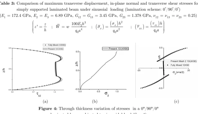
simply supported laminated beam (with S = 4 and 10) have been presented in Table 3. Results obtained through present analysis are compared with elasticity solution by Pagano (1969) and various analytical/ FE solutions given by Desai and Ramtekkar (2002); Lo et al. (1978); Spilker (1982); Engblom and Ochoa (1985); Toledano and Murakami (1987); Manjunatha and Kant (1993b). Present results shows good agreement with the elasticity solutions, which underlines the usefulness of the present model. Variation of normalized longitudinal normal stress (σ_x) and

transverse stresses (σ_z and τ_xz) through thickness of beam with S = 4 is presented in Fig. 3. It is

(11)

S Source σ_X

(

a 2,h 2

)

σ_X

(

a 2,−h 2

)

τ_XZ(max) W

(

a 2, 0

)

4

Pagano (1969) 18.6102 -18.0023 1.5974 2.8600

Lo et al. (1978) - - 1.5555 -

Spilker (1982) - - 1.5636 2.8410

Engblom and Ochoa (1985) 10.0090 -10.1081 1.7734 -

Toledano and Murakami (1987) - - - 2.8810

10

Pagano (1969) 73.6000 -73.2000 4.2346 0.9568

Spilker (1982) - - 4.5292 0.9312

Engblom and Ochoa (1985) 63.7344 -63.4025 4.4590 -

Note: (i) ‘−_{’ represents result not available}

Table 3: Comparison of maximum transverse displacement, in-plane normal and transverse shear stresses for simply supported laminated beam under sinusoial loading (lamination scheme: 0°_/90°_/0°₎

1 2 3 12 13 23 12 13 23

(E =172.4 GPa, E =E = 6.89 GPa, G =G =3.45 GPa, G =1.378 GPa, ν = ν =ν = 0.25)

( )

(

)

(

)

2 3

2

4 2

0

0 0

100

' z ; E h ; _x x h ; _xz xz h

z W w

h q a q a q a

σ τ

 _

 _

 = = = = 

 _

 

 

0.0 0.5 1.0

-0.5 0.0 0.5

z

/h

σ

z

Present 10/(4X90)

(a) (b) (c)

Figure 4: Through thickness variation of stresses in a 0°/90°/0° laminated beam subjected to sinusoidal load (S = 4)

(

)

(

)

( )

(

)

(a) τ_xz 0,z , (b) σ_z a 2,z , c σ_x a 2,z

3.2 Free vibration analysis

3.2.1 Example 3

A six-layer symmetric cross-ply (0°/0°/90°/90°/0°/0°) thick beam under simple support is

(12)

the present model are compared in Table 4 with FOBT, HOBT by Marur and Kant (1996), mixed theory by Rao et al. (2001) and FEM solution by Ramtekkar et al. (2002). The through thickness variation of non dimensional inplane displacements, transverse normal and shear stresses for first three modes is shown Fig. 5. It can be observed that the results from the present studies are in good agreement with HOBT and the mixed theory with a substantial reduction in the total DOF.

Mode Marur and Kant(1996) Rao et al.

(2001)

Ramtekkar et.al (2002)

Present Mesh 1 10/(2X90)

Present Mesh 2 10/(2X90)

FOBT HOBT

1 1.639 1.6540 1.655 1.657 1.656 1.655

2 3.810 3.9160 1.879 3.910 3.918 3.919

3 5.912 6.1800 3.908 6.138 6.180 6.187

4 7.988 8.4460 6.146 8.323 6.422 8.440

5 10.100 10.7110 8.400 10.440 8.447 10.725

6 11.181 12.9690 10.694 12.469 10.716 11.109

7 12.188 15.2220 11.107 14.385 11.109 12.531

8 12.953 17.4690 12.616 16.161 12.987 12.970

9 14.392 19.7120 13.061 17.771 15.261 15.290

10 16.732 - 15.510 - 17.524 17.494

11 19.088 - 17.404 - 17.808 18.875

12 19.205 - 18.837 - 18.900 19.980

13 - - 20.168 - 19.765 22.104

14 25.910 - 21.639 - 22.093 22.988

15 - - - - 24.338 24.857

Table 4: Comparison of non-dimensional natural frequencies

₍

2

₎

1

a h E

ω = ω× × ρ

of (0/0/90/90/0/0) simply supported beam

(E₁=525 GPa, E₂ =21 GPa, G₁₂ =10.50 GPa, ν₁₂ =0.3, Density (ρ)= 800 Ns2/m4, Length = 762 mm, Breadth = 25.4 mm, Depth = 152.4 mm)

(a) (b) (c)

(13)

Latin American Journal of Solids and Structures 12 (2015) 2061-2077 3.2.2 Example 4

A six-layer un-symmetric cross-ply (0°/90°/0°/90°/0°/90°) thick beam under simple support

condition is considered in this example. The non-dimensional natural frequencies (ω) for different

modes have been presented in Table 5. Comparison of frequencies with the available results from FOBT, HOBT (4a, 4b, 5) by Marur and Kant (1996), mixed theory by Rao et al. (2001) and FEM solution by Ramtekkar et al. (2002) has been done. The results show good agreement with the earlier reported results in the literature.

Mode Ramtekkar et al. (2002)

Marur and Kant (1996)

HOBT5 Present

Mesh 1

Present Mesh 2 10/(4X90)

FOBT HOBT4a HOBT4b

1 1.376 1.432 1.483 1.434 1.416 1.384 1.415

2 2.791 3.597 3.806 3.614 3.531 3.509 3.522

3 3.480 5.750 6.153 5.870 5.675 5.431 5.667

4 5.577 7.856 8.457 8.114 7.795 5.687 7.766

5 7.696 9.994 10.809 10.462 10.021 7.759 9.934

6 9.887 10.932 10.935 10.762 10.668 9.897 10.646

7 11.107 11.181 12.248 11.110 11.110 11.109 11.109

8 11.597 12.104 13.132 12.807 12.285 12.067 12.109

9 12.189 14.319 15.575 15.253 14.633 14.254 14.324

10 14.062 15.868 16.468 15.839 15.663 15.1055 15.632

11 15.871 16.673 18.166 17.873 17.244 16.463 16.467

12 16.178 19.147 20.889 20.611 19.981 16.686 18.924

13 19.294 - 21.709 21.430 21.108 18.677 21.011

14 20.314 21.855 - - - 20.991 21.022

15 - - - 22.069 22.746

₍

2

₎

1

a h E

ω = ω× × ρ of a simply supported

thick un-symmetrically laminated composite beam (0o/90o/0o/90o/0o/90o)

(E₁ =525 GPa, E₂ =21 GPa, G₁₂ =10.50 GPa, ν₁₂ =0.3, Density (ρ)= 800 Ns2/m4, Length = 762 mm, Breadth = 25.4 mm, Depth = 152.4 mm)

3.2.3 Example 5

A symmetric cross-ply (0°_/90°_/90°_/0°_{) thin beam under simple support condition is considered for}

free vibration analysis. The non-dimensional natural frequencies (ω) obtained from the present

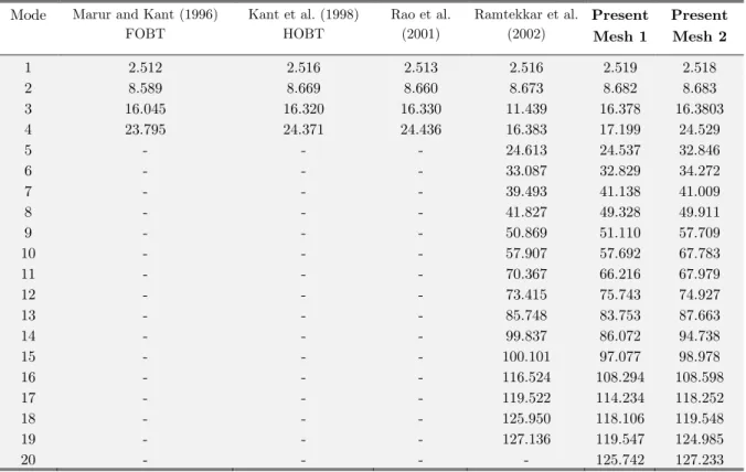
investigation are compared in Table 6, with the first order beam theory FOBT (4a) by Marur and Kant (1996), HOBT by Kant et al. (1998) and the mixed theory by Rao et al. (2001) and FEM solution by Ramtekkar et al. (2002). Results have been observed to be in very good agreement with the HOBT and the mixed theory.

3.2.4 Example 6

A four layered angle ply beam with layup (θ°/-_θ°/-_θ°/_θ°) is considered in this example. To

(14)

Mode Marur and Kant (1996) FOBT

Kant et al. (1998) HOBT

Rao et al. (2001)

Ramtekkar et al. (2002)

Present Mesh 1

Present Mesh 2

1 2.512 2.516 2.513 2.516 2.519 2.518

2 8.589 8.669 8.660 8.673 8.682 8.683

3 16.045 16.320 16.330 11.439 16.378 16.3803

4 23.795 24.371 24.436 16.383 17.199 24.529

5 - - - 24.613 24.537 32.846

6 - - - 33.087 32.829 34.272

7 - - - 39.493 41.138 41.009

8 - - - 41.827 49.328 49.911

9 - - - 50.869 51.110 57.709

10 - - - 57.907 57.692 67.783

11 - - - 70.367 66.216 67.979

12 - - - 73.415 75.743 74.927

13 - - - 85.748 83.753 87.663

14 - - - 99.837 86.072 94.738

15 - - - 100.101 97.077 98.978

16 - - - 116.524 108.294 108.598

17 - - - 119.522 114.234 118.252

18 - - - 125.950 118.106 119.548

19 - - - 127.136 119.547 124.985

20 - - - - 125.742 127.233

₍

2

₎

1

a h E

ω= ω× × ρ of a simply supported thick un-symmetrically laminated composite beam (0o/90o/90o/0o)

(E₁=1.448x108 kN/mm2, E₂ =9.65x106 kN/mm2, G₁₂ =4.14x106 kN/mm2,, ν₁₂ =0.3, Density (ρ)= 1839.23 Ns2/m4, Length = 15 m, Breadth = Depth = 1 m)

BC Source

Ply angle 'θ°_'

0° 15° 30° 45° 60° 75° 90°

SS Adyodgu (2006) 2.651 1.896 1.141 0.804 0.736 0.725 0.729

Present Mesh 1 (10/(3x60)) 2.615 1.386 0.749 0.721 0.731 0.705 0.731

Present Mesh 2 (10/(2x60)) 2.614 1.386 0.749 0.720 0.730 0.705 0.730

CC Adyodgu (2006) 4.973 4.294 2.195 1.929 1.669 1.612 1.619

Present Mesh 1 (10/(3x60)) 4.676 2.906 1.662 1.604 1.628 1.577 1.632

Present Mesh 2 (10/(2x60)) 4.670 2.903 1.659 1.601 1.624 1.573 1.628

CF Adyodgu (2006) 0.981 0.676 0.414 0.288 0.262 0.258 0.260

Present Mesh 1 (10/(3x60)) 0.973 0.500 0.268 0.258 0.261 0.252 0.261

Present Mesh 2 (10/(2x60)) 0.973 0.500 0.268 0.257 0.261 0.252 0.261 FC Present Mesh 1 0.973 0.500 0.268 0.258 0.261 0.252 0.261

Table 7: Variation of non-dimensional fundamental frequency

₍

2

₎

1

a h E

ω = ω× × ρ of a four layer angle ply laminated beam (θ°_/₋_θ°_/₋_θ°_/_θ°_{) under different boundary conditions (BC).}

(15)

Latin American Journal of Solids and Structures 12 (2015) 2061-2077 for θ =0°, 15°, 30°, 45°, 60°, 75°, 90°. Simply supported at both ends (SS), clamped at both ends

(CC) and clamped free (CF) boundary conditions are considered. CF condition with Mesh 1 meshing pattern has a stack of 2D mixed elements at the clamped end and remaining domain is modelled with HOSTB8 elements. An end condition, free clamped (FC) is also considered with Mesh 1 meshing pattern having the stack of 2D mixed elements at the free end. The non-dimensional fundamental frequencies are compared with those presented by Adyodgu (2006) in Table 7. Variation of the fundamental frequency with the ply angle for boundary condition (SS) is shown in Fig 6. Except for θ=15° and 30°, natural frequencies for all other orientation of plies are in

close proximity of those presented by Adyodgu (2006). The consistency between results of the two meshing patterns under all boundary conditions strengthens the efficacy of the combined mesh model.

Figure 6: Variation of non-dimensional fundamental frequency of a four layer angle ply SS beam (θ°/-_θ°/-_θ°/_θ°) with ply angle.

The results of above examples illustrate that the present multi-modelling scheme is apt for complete analysis of laminated beams. The accuracy requirements are fulfilled without sacrificing the computational efficiency. Continuity of transverse stresses is also ensured. It is observed that Ramtekkar et al.(2002) presented few frequencies which were not reported earlier in the literature. Present combined mesh model misses out on few of those additional frequencies reported in Ramtekkar et al. (2002) but on the other hand some new frequencies are encountered. The genuineness of these new frequencies is under investigation by the authors.

4 CONCLUSION

(16)

to reduction in number of elements rquired for the entire domain. This makes the procedure computationally economical. Increase in the size of the local LW mixed sub-domain would make the mesh to tend towards full LW modeling and the methodology may loose its advantage. An accuracy above 90% in comparison with elasticity solution is seen to be achieved by using LW mixed model on 25% to 40% of the entire domain. The present combined formulation overcome the shortcoming of ESL in prediction of continuity of the transverse stresses. The method suggested is confirming to the elasticity principles as both the models used on the sub-domains are derived from the elasticity equations and two dimensional state of stress and strain. The results given by the developed model show reasonably good accuracy as compared with the benchmarks from the literature.

References

Adyodgu, M., (2006). Free Vibration Analysis of Angle-ply Laminated Beams with General Boundary Conditions. J. Reinforced Plastics and Composites 25(15): 1571-1583.

Bathe, K.J., (1997). Finite element procedures. New Delhi: Prentice-Hall of India.

Cook, R.D., Malkus, D.S., Plesha, M.E., Witt, R.J., (2003). Concepts and applications of finite element analysis. Fourth edition, John Willey & Sons (Asia): 278-279.

Desai, Y.M., Ramtekkar, G.S., (2002). Mixed finite element model for laminated composite beams. Structural Engineering and Mechanics 13(3): 261-276.

Engblom, J.J., Ochoa, O.O., (1985). Through the thickness stress predictions for laminated plates of advanced composite materials. Int. J. Numerical Methods in Engineering 21: 1759-1776.

Kant, T., (1982). Numerical analysis of thick plates. Computer methods in Applied Mechanics and engineering 31(1): 1-18.

Kant, T., Marur, S.R., Rao, G.S., (1998). Analytical solution to the dynamic analysis of laminated beams using higher order refined theory. Composite Structures 40(1): 1-9.

Liou, W.J., Sun, C.T., (1987). A three-dimensional hybrid stress isoparametric element for the analysis of laminated composite plates. Computers & Structures 25(2): 241-249.

Lo, K.H., Christensen, R.M., Wu, E.M., (1978). Stress solution determination for high order plate theory. Int. J. Solids and Structures 14: 655-662.

Lu, X., Liu, D., (1992). An interlaminar shear stress continuity theory for both thin and thick composite laminates. ASME J. Applied Mechanics 59: 502-509.

Manjunatha, B.S., Kant, T., (1993a). New theories for symmetric/unsymmetric composite and sandwich beams with C0 finite elements. Composite Structures 23: 61-73.

Manjunatha, B.S., Kant, T., (1993b). Different numerical techniques for the estimation of multiaxial stresses in symmetric/unsymmetric composite and sandwich beams with refined theories. J. Reinforced Plastics and Composites 12: 2-37.

Marur, S.R., Kant, T., (1996). Free vibration analysis of fiber reinforced composite beams using higher order theories and finite element modelling. J. of Sound and Vibration 194(3): 337-351.

Marur, S.R., Kant, T., (2007). On the angle ply higher order beam vibrations. Computational Mechanics 40(1): 25-33.

Pagano, N.J., (1969). Exact solutions for composite laminates in cylindrical bending. J. Composite Materials 3: 398-411.

(17)

Pagano, N.J., Hatfield, S.J., (1972). Elastic behavior of multilayered bi-directional composites. AIAA J. 10: 931-933.

Pipes, R.B., Pagano, N.J., (1970). Interlaminar stresses in composite laminates under uniform axial extension. J. Composite Materials 4(4): 538-548.

Ramtekkar, G.S., Desai, Y.M., Shah, A.H., (2002). Natural vibrations of laminated composite beams by using mixed finite element modelling. J. Sound and Vibration 257(4): 635-651.

Rao, K.M., Desai, Y.M., Chitnis, M.R., (2001). Free vibrations of laminated beams using mixed theory. Composite Structures 52(2): 149-160.

Reddy, J.N., (1987). A generalization of two-dimensional theories of laminated composite plates. Commun. Applied Numerical Methods 3: 173-180.

Rybicki, E.F., (1971). Approximate three-dimensional solutions for symmetric laminates under in-plane loading. J. Composite Materials 5: 354-360.

Shimpi, R.P., Ghugal, Y.M., (1999). A layerwise trigonometric shear deformation theory for two layered cross-ply laminated beams. J. Reinforced Plastics and Composites 18: 1516-1543.

Spilker, R.L., (1982). Hybrid‐stress eight‐node elements for thin and thick multilayer laminated plates. J. Numerical Methods in Engineering 18(6): 801-828.

Srinivas, S., Rao, A.K., (1970). Bending, vibration and buckling of simply supported thick orthotropic rectangular plates and laminates. J. Solids and Structures 6(11): 1463-1481.