Lat. Am. j. solids struct. vol.12 número11

(1)

Abstract

The use of thin-walled composite beams in Engineering has at-tracted great interest in recent years. Composite beams and other structural elements tend to have thin walls due to the high strength of the material. Other important aspect is that, even without reach-ing large strains and without overcomreach-ing the elastic limit of the material, such as beams present geometric nonlinear behavior due to their high slenderness, leading to large displacements and rota-tions. In this paper, a three-dimensional frame finite element for geometric nonlinear analysis of thin-walled laminated composite beams is presented. The finite element uses the Total Lagrangian formulation in order to allow the treatment of large displacements, but with moderated rotations. The constitutive matrix of the lami-nated beams is evaluated through a suitable thin-walled beam the-ory. In this theory, the effects of the couplings for several layups are considered, but the effects of the warping and transverse shear are neglected. Comparisons with numerical experiments demonstrate the very good accuracy of the proposed finite element.

Keywords

Composite materials; thin-walled beams; three-dimensional frame finite element; geometric nonlinearity.

Geometrically nonlinear analysis of thin-walled laminated

composite beams

1 INTRODUCTION

The use of thin-walled laminated composite beams in Aeronautical, Mechanical, Naval and Civil Engineering has attracted great interest in recent years due to several advantages of fiber reinforced composite materials, such as high specific strength and stiffness, high corrosion resistance, good thermal insulation, excellent damping properties and fatigue resistance. Other important character-istic is that, even without reaching large strains and without overcoming the elastic limit of the material, such beams present geometric nonlinear behavior due to high slenderness, leading to

Luiz Antônio Taumaturgo Mororóa Antônio Macário Cartaxo de Melob Evandro Parente Juniorc

Laboratório de Mecânica Computacional e Visualização, Departamento de Engenharia Estrutural e Construção Civil,

Universidade Federal do Ceará.

Corresponding author: a_{luiztaumaturgo@gmail.com} b_{macario@ufc.br}

c_{evandro@ufc.br}

http://dx.doi.org/10.1590/1679-78251782

(2)

Latin American Journal of Solids and Structures 12 (2015) 2094-2117

large displacements and rotations. Obviously, the analysis and design of these beams require the use of appropriated theoretical and computational tools.

In laminated composites, each ply presents orthotropic behavior, where the fiber direction is stronger and stiffer than the orthogonal directions. On the other hand, laminated composites can present anisotropic behavior, due to the presence of plies with different orientations, leading to cou-plings between forces and strains that are not present in isotropic beam case.

A more natural option to the structural analysis of thin-walled laminated composite beams is the use of shell or solid finite elements, in which orthotropic materials with different orientations in each ply and effects due to transverse shear deformation and warping can readily be defined. In addition, these elements provide directly stresses in each ply. However, the computational cost and the mesh and geometry generation processes of this approach are prohibitive, except for small structures. Such issues increase significantly when geometric nonlinear effects are considered.

Therefore, the development of three-dimensional frame finite element for geometric nonlinear anal-ysis of thin-walled laminated composite beams is an attractive task, due to low mesh and geometry generation as well as low computational cost. Several studies addressing this issue have been developed in recent years and Total and Updated Lagrangian approaches are usually used.

Bhaskar and Librescu (1995) proposed a finite element based on Total Lagragian theory taking into account the effects due to transverse shear deformation and warping to analyze thin-walled anisotropic beams with closed and open sections. In the same way, Vo and Lee (2009a) proposed a three-dimensional frame finite element based on Von Kármán strain tensor to analyze laminated box beams. The effects of the composite layup and couplings were assessed. After, the authors enhanced such finite element to consider transverse shear deformation effects (Vo and Lee, 2010a). Cardoso et al. (2009); Omidvar and Ghorbanpoor (1996) proposed a three-dimensional frame finite element based on Updated Lagrangian theory to analyze thin-walled laminated beams including warping effects. In these works, the authors analyzed only beams with open-section.

In this paper, a three-dimensional frame finite element for geometric nonlinear analysis of thin-walled laminated composite beams is presented. The finite element uses the Total Lagrangian formu-lation in order to allow the treatment of large displacements, but with moderated rotations. In this formulation, the constitutive matrix of the laminated beams is evaluated through the Kollar and Pluzsik (2002) theory. In this theory, the effects of the couplings for several layups are considered, but the effects of the warping and transverse shear are neglected.

Numerical applications are accomplished in order to verify the performance of the proposed ele-ment formulation. Verification is carried out through shell three-dimensional finite eleele-ment models developed in the ABAQUS (Simulia, 2012) commercial software and numerical simulations found in the literature. A very good agreement was obtained between the results of the proposed finite element and computational results available in the literature, as well as the results of shell models analyzed using ABAQUS.

2 BEAM THEORY

(3)

Latin American Journal of Solids and Structures 12 (2015) 2094-2117 Considering arbitrary layup and arbitrary cross-section, and neglecting the effects due to trans-verse shear deformation and to warping, the constitutive relation for thin-walled laminated composite beams can be given by (Kollar and Pluzsik, 2002):

11 12 13 14 21 22 23 24 31 32 33 34 41 42 43 44

x x

y y

v v v

z z

N C C C C

M C C C C

T C C C C

ε κ κ β

     

   

    

  _ _ 

   

 ₌  _⇒ ₌

  _ _ 

  _ _ 

   

  _ _ 

   

    

   

     

C

σ ε (1)

where N_x is the axial force, M_y and M_z are the bending moments about y and z axes, respectively,

T is the torque, ε_x is the normal strain in the x direction, κ_y and κ_z are the beam curvatures about y and z axes, respectively, β is the rate of change of twist angle along x direction (Figure

1), C_v is the constitutive matrix of the beam, which coefficients represent the beam section properties.

Figure 1: Beam forces and global coordinate system.

For a isotropic beam with doubly symmetric cross-section, the relationships in Equation (1) based on Euler-Bernoulli-Navier and Saint Venant theories are uncoupled (C₁₁ =EA, C₂₂ =EI_y, C₃₃ =EI_z,

44

C =GJ ):

0 0 0

x x

y y y

z z z

N EA

M EI

T GJ

ε κ κ β

     

   

    

  _ _ 

   

 ₌  

  _ _ 

  _ _ 

   

  _ _ 

   

    

   

     

(2)

(4)

matrix becomes 7x7 (Sheikh and Thomsen, 2008). In addition, it can be found in literature 8x8 (Vo and Lee, 2008; Vo and Lee, 2009a) and 9x9 (Salim and Davalos, 2005; Vo and Lee, 2011) C_v matrices to assess box and open cross-section beams.

It is important to note that formulation and boundary conditions of the problem become more difficult as much as the improvements of the theory (approach) to obtained constitutive beam matrix. In addition, the computational efforts are increased, due to great number of degrees of freedom. Cesnik and Hodges (1997) developed a two-dimensional finite element model, implemented in VABS (Variational Asymptotical Beam Sectional Analysis) software, for predict laminated beam section properties. Such approach is based on the called method VAM (Variational Asymptotical Method). This method splits the three-dimensional model in two ones: a two-dimensional one over the cross-section and another along length.

In order to assess the several effects, especially due to shear deformation and warping, Volovoi et al. (2001) analyzed many thin-walled laminated beam theories. According to Volovoi et al. (2001), in many practical cases a C_v 4x4 matrix well formulated leads to good results mainly for closed cross-section. Using a more refined theory for this case, the gain is small. According to Volovoi et al. (2001), the effects due to shear deformation and warping are not important for beams with closed cross-section. Pluzsik and Kollar (2002) presented the same conclusion using shell element.

There are many approaches to assess thin-walled composite beams considering open and closed sections. Since the focus of this work is closed sections and based on the results and conclusions of Volovoi et al. (2001); Pluzsik and Kollar (2002), the approach proposed by Kollar and Pluzsik (2002) is used to predict the constitutive matrix.

2.1 Kollar and Pluzsik theory

Kollar and Pluzsik (2002) proposed a general theory to analyze thin-walled laminated beams and presented analytical expressions for constitutive matrix C_v for open and closed sections. Considering a closed section, the beam’s wall consists of N flat segments each one may be made of several layers of composite materials with arbitrary layup (Figure 2).

As indicated in Figure 3, the following coordinate system are employed: x y z global coordinate

system with origin at the mechanical centroid (point C); x y z global coordinate system with origin

at an arbitrary chosen point (point O); x s r_i _{i i} local coordinate system for the -th segment with origin at the center of reference plane of the -th segment (point c_i). The x_i axes is parallel to the

x coordinate, the s_i axes is along the segment and r_i is normal to the segment.

According to Classical Laminated Theory (CLT) the strain-stress relationship in the i-th segment may be given by (Jones, 1999; Reddy, 2004):

(5)

Latin American Journal of Solids and Structures 12 (2015) 2094-2117 Figure 2: Segments of the cross-section. Figure 3: Coordinate systems.

The displacements of the centroidal axes are the axial displacement u, the transverse displacements vand w in the y and z directions, respectively, and rotation of the cross-section ψ (twist angle). Considering the convention of positive internal forces as showed in Figure 1, the relationships between these displacements and strains at the global system x y z are:

2 2

d d d d

; ; ;

d d d d

x y z

u w v

x x x x

ψ

ε = κ = − κ = β= ₍₄₎

In the global system x y z these relationships become:

2 2

d d d d

; ; ;

d d d d

x y z

u w v

x x x x

ψ

ε = κ = − κ = β = (5)

Where ε_x , κ_y, κ_z and β are the axial strain, curvatures and twist rate of the longitudinal axes passing through the origin of the coordinate system x y z , respectively; u, w, v and ψ are the displacements of the x axis.

2.2 Closed cross-section

When a closed section beam is cut lengthwise, the cut edges are subjected to relative displacements as shown in Figure 4. These displacements are prevented in the original beam by means of generalized forces X₁, X₂, X₃ and X₄. The transverse forces X₃ and X₄ along cut edges are generally neglected

(Kollar and Pluzsik, 2002). The shear force X₁ and bending moment X₂ correspond to N_xs and M_s

in Equation (3), respectively. These terms do not change along cut edges.

Compatibility equations along the edges must be used to predict X₁ and X₂ (Kollar and Pluzsik,

2002):

left right

o o

u u

w w

s s

=

∂ ∂

=

∂ ∂

(6)

Figure 4: Cut of the closed section beam. Figure 5: Rotation in cut beam.

where _wo_{is the displacement of the wall perpendicular to the segment’s reference surface (Figure 5).} The first compatibility equation can be express as:

2Aβ γ_xso ds 0

− +

_∫

= ₍₇₎

where A is the enclosed area of the cross-section defined by middle surface and o xs

γ is the shear strain of the segment at its plane.

The second compatibility equation can be written by using the definition 2 o 2

s w s

κ = −∂ ∂ . In this case, the second relationship in Equation (6) becomes:

d 0

s s

κ =

∫

(8)

In order to analyze thin-walled closed section composite beams, Kollar and Pluzsik (2002) define the following five steps that must be done:

1. The strains in each segment of the beam cross-section are related to the axial strain, curvatures and twist of the longitudinal beam axis through kinematic hypothesis and plate theory.

2. The forces X₁ and X₂ in each segment of the beam cross-section are expressed in terms of strains

in the segments.

3. The resultant axial force, bending moments and torque acting at the longitudinal axis of the beam are determined from the segment forces.

4. X₁ and X₂ are determined from compatibility equations.

5. The constitutive matrix C_v is established by relating the resultant axial force, bending moments and torque to the axial strain, curvatures and angle of twist of the longitudinal beam axis.

After all the steps have been done in conjunctions with compatibility equations, the constitutive matrix can be written as (Kollar and Pluzsik, 2002):

(

1

)

1

1 N

t t

v i i i

i

C − −

=

(7)

Latin American Journal of Solids and Structures 12 (2015) 2094-2117 where,

11 11 16

2 11

16 16 66

1 0 2 1 0 1 2 12

0 0 0

1 1 1

0

2 2 4

i i

i i b

a b

α β β

β δ δ

   −       ₋      = _ _         − −      ω (10)

The coefficient a₁₁_i is computed by:

1 11 12 13 11 11 16 12 22 23 11 11 16 13 23 33 _i 16 16 66 _i

a a a a a a a a a

α β β

β δ δ

−           ₌                   (11)

The matrixes F and L are respectively given by:

16 12

61 12

16 61 66

66 62 1

62 22 1

12 12 26

66 26 1 0 2 0 0 1

0 ₁ ₁

2 2 2 N i i i _i i i b α β β δ

α β β

α β β δ

β δ δ

β δ − =   _{ }  _ _{ }             −    _ _     _ _ _ _{ }  = _{ } _ _{− } _ _ _{ }_          −               _− − _     _ _ 

∑

F ω (12)

0 0 0 2 0 0 0 0 A  −    = _ _−    

L J ₍₁₃₎

where,

16 61 66

1 1

12 12 26

1 0 2 1 0 2 N i i i i

α β β

β δ δ

− =    −    = _ _  ₋     

∑

J ω R (14)

The matrix R_i can be written through the relationship between the strains of the axis of the i -th segment:

1 0

0 cos sin 0 0 sin cos 0

0 0 0 1

i

c

x i i x

c

s i i y

c

i i z

r c

i

z y

ε ε

κ α α κ

α α κ

(8)

where z_i and y_i are the origin coordinates of the x s r local system for the i-th segment (Figure 6). The angle α_i is the angle between the s and y axes (Figure 6). The superscript c refers to the

longitudinal axis passing through middle of the average surface of the segment (s = 0 and r =0). The first of these equations is written according to Euler-Benoulli-Navier hypothesis. The quantities

c si

κ and κ_ric are the curvatures of the i-th segment in the x r and x s plane, respectively (Figure 7).

The last equation is written considering that the angle of twist of the wall segment is equal to the angle of twist of the beam ( c

i

β =β).

Kollar and Pluzsik (2002) and Mororó (2013) present the detailed formulation. In this work, the axis orientations are the same ones adopted by Mororó (2013).

Figure 6: Coordinates of point c_i and segment orientation (angle α).

Figure 7: Axis curvatures in the i-th segment.

The previous formulation was focused on closed cross-section. Nonetheless, it is worth to em-phasize that for open cross-section, the forces and are neglected. Then, from Equation (9) the constitutive matrix for this case is given by (Kollar and Pluzsik, 2002):

(

1

)

1 N

t

v i i i

i

−

=

∑

(9)

Latin American Journal of Solids and Structures 12 (2015) 2094-2117 3 FINITE ELEMENT FORMULATION

The element formulation is based on the Bernoulli-Euler-Navier bending hypothesis and the Saint Venant’s torsion hypothesis. As shallow arch approach is used, the geometric nonlinearity is consid-ering only in the axial strain:

2 2

, , ,

, ,

1 1

2 2

x x x x

xy y x xz z x

u v w

u v

u w

ε

γ γ

= + +

= +

(17)

where u, v and w are the local displacements of a generic point P of the cross-section (Figure 8

).

They can be written as:

, ,

c c x c x c x

c x

u u yv zw v v z

w w y

θ

= − −

= −

= +

(18)

where u_c, v_c and w_c are the displacement components of the centroid of the cross-section and θ_x is the rotation about the x axis.

Figure 8: Displacement of generic point P on the cross-section.

Substitution of Equation (18) in Equation (17) yields:

, , , ,

, ,

x m z y c x x x c x x x xy x x

xz x x

y z yw zv

z y

ε ε κ κ θ θ

γ θ

= − + + −

= −

=

(19)

(10)

(

)

2 2 2 2 2

, , , ,

, ,

1 1 1

2 2 2

m c x c x c x x x

y c xx z c xx

u v w y z

w v ε θ κ κ = + + + + = − = (20)

In this element, the nonlinearity is only considered in membrane part εm (shallow arch), as considered by MacGuire et al. (2000). Then, the two last terms (yw_{c x x x}_, θ_, and zv_{c x x x}_, θ_, ) of the axial strain defined in Equation (19) will be neglected. In the following, the subscript c will be dropped to simplify the

notation, since only displacements of centroid appear in Equation (20).

Using the Principle of Virtual Work (PVW), the internal virtual work (δU ) is given by:

(

_x _x _xy _xy _xz _xz

)

d V

U V

δ =

∫

σ δε +τ δγ +τ δγ ₍₂₁₎

Using Equation (19):

(

x m x z x y xy x x, xz x x,

)

d d

L A

U y z z y A x

δ =

∫ ∫

σ δε − σ δκ + σ δκ − τ δθ + τ δθ

(22)

where A and L are cross-section area and element length, respectively.

Noting that only the last term in ε_m varies with respect to A and assuming an average normal

stress so that σ_x =N_x A (MacGuire et al., 2000; Battini and Pacoste, 2002; Battini, 2002), the first term of Equation (22) becomes:

2 2 2

, , , ,

1 1

d d d

2 2 2

p

x m x x x x x x

L A L

I

A x N u v w x

A

σ δε δ θ

 _  _  = __ + + + _   

∫ ∫

∫

(23)

where I_p is the polar moment of inertia of the cross-section:

(

2 2

)

_d

p A

I =

∫

y +z A ₍₂₄₎

Integration of the second and third terms in the Equation (22) over the cross-section leads to bending moments about z and y axes, respectively:

d d z x A y x A

M y A

M z A

σ σ = − =

∫

(25)

Finally, the integration over the cross-section of the last two terms in the Equation (22) leads to:

(

)

d 1 d xy A xz A

z A T

y A T

(11)

Latin American Journal of Solids and Structures 12 (2015) 2094-2117 where the portions

(

α−1

)

and α of the total torsion moment T are resisted by mean of the stresses

xy

τ and τ_xz, respectively. For Saint Venat’s pure torsion, α=1 2 (MacGuire et al., 2000). Therefore, Equation (22) becomes:

(

x m y y z z x x,

)

d

L

U N M M T x

δ =

∫

δε + δκ + δκ + δθ

(27)

From PVW, the internal virtual work can be written as:

d

t t

v v L

x δd g=

∫

δε σ

(28)

where g and δd are internal nodal force vector and virtual nodal displacement vector, respectively;

v δε and

v

σ are the virtual generalized strain vector and the generalized stress vector, respectively. The generalized beam strains are written in terms of degrees of freedom of element by:

v v δ δ = = Bd B d ε ε (29)

where

{

,

}

t v = εm κy κz β = θx x

ε , B is the displacement-strain matrix and B is the matrix that relates the variation of the strains to variation of the displacements. The next steps of the for-mulation are devoted to the determination of B and B matrices.

In order to avoid membrane locking due to unbalanced of the axial and transverse terms, the average membrane strain (Crisfield, 1991; Battini and Pacoste, 2002; Battini, 2002) is used for ε_m:

2 2 2

, , , ,

0

1 1 1

d

2 2 2

L

p

m x x x x x

I

u v w x

L A ε θ  _  _  = __ + + + __  

∫

(30)

Solving the above integral, the average membrane strain can be expressed as:

2 1 2 2 2

, , ,

0 0 0

1 1

d d d

2 2 2

L L L

p

m x x x x

I u u

v x w x x

L L L LA

ε = − +

∫

+

∫

+

∫

θ (31)

where u₁ and u₂ are the element nodal displacements at the nodes 1 and 2, respectively.

After discretization, the displacements in the element are interpolated from nodal displacements (nodal degrees of freedom). Let m be the degree of the higher-order derivative in PVW equation, the

interpolation function must have _Cm−1_{continuity for adjacent elements. Therefore, function with} 0

C continuity can be used to interpolate the axial displacement and the twist angle and the transverse

displacements require the use of functions with _C1 _continuity: 2 1

1, 2, 0

, 1, 2, 3, 4, ,

, 1, 2, ,

0 0 0 0 0 0 0 0 0 0

0 0 0 0 0 0 0 0

0 0 0 0 0 0 0 0 0 0

x x

x x x x x bv x

x x x x x bw x

x x x x x

u u

N N

L

v H H H H

w H H H H

N N _θ

θ − _ _ = __ __ =   =__ __ =   =__ − − __ =   =__ __ =

d B d

d B d

(12)

where d is the vector of nodal displacements, N_i are the linear Lagrange polynomials and H_i

func-tions are the Hermite (cubic) polynomials:

Using Equation (32), the average membrane strain can be written in matrix form as:

(

)

0

1 1 1

2 2 2

1 2

L

m Lv Lw L

m L m m θ θ ε ε ε ε = + + +     =_ + + + _      _  =_ + __   = B

B d B d B d B d

B B B B d

B B d

B d (33) where , , 0 , , 0 , , 0 d d d L t t

Lv v v bv x bv x L

t t

Lw w w bw x bw x L

t t

L x x

x x x

θ θ θ θ θ

= ⇒ = = ⇒ = = ⇒ =

∫

B d A A B B

(34)

The bending curvatures κ_y and κ_z and twist rate θ_{x x}_, are the same ones used in traditional linear three-dimensional frame element (MacGuire et al., 2000). Then, from Equations (20), (32) and (33), the nonlinear B matrix is given by:

0 , , , , , , 1 2 0 0 0 m L

bw xx bw xx bv xx bv xx

x x θ θ       _ _     _ _     _ _     _ _ =_ _= _ _+_ _     _ _     _ _     _ _     _ _

B B B

B B

B

B B

(35)

The membrane strain variation δε_m is obtained from Equation (33):

(

) (

)

0 0

1 2

m L L L

m m

δε δ δ δ δ

δε δ

= + + = +

=

B d B d B d B B d B d

(36)

Using Equations (20) and (32) it can show that:

0 , , , , , , 0 0 0 m L

bw xx bw xx bv xx bv xx

x x θ θ                         =_ _ =_ _+_ _                        

B B B

B B

B

B B

(13)

Latin American Journal of Solids and Structures 12 (2015) 2094-2117 Using Equations (28) and (29), the element internal force vector (g) is given by:

d t

v L

x =

_∫

g Bσ

(38)

The use of quadratically convergent Newton-Rapshon method to solve the nonlinear equilibrium equations requires the computation of the tangent stiffness matrix. The tangent stiffness matrix (K_T) is obtained by differentiation of the internal force vector with respect to the nodal displacements:

d d

t t v

T v E G

L L

x x

∂

∂ ∂

= = + = +

∂

∫

∂

∫

∂

g B

K B K K

d d d

σ

σ (39)

where K_E is the elastic stiffness matrix and K_G is the geometric (or initial stress) stiffness matrix. Remembering that σ_v =C_{v v}ε and using the second relationship in Equation (29), the elastic stiffness matrix can be expressed as:

d t

E v

L

x =

_∫

K B C B ₍₄₀₎

Using Equations (33), (34), (34) and (37), the term ∂ ∂B d can be written as:

(

)

0 0 0

L

L t t t

v w θ v w θ

∂ 

 

 _∂ 

  _∂

∂ _ _ ∂

=_ _ ⇒ = + + = + + =

∂ _ _ ∂ ∂

 

 

B d

B B

d A d A d A A A A A

d d d (41)

Therefore, the geometric stiffness matrix is given by:

d t

G x

L

N x =

_∫

K A ₍₄₂₎

It is important to note that, differently from the standard beam elements, the normal force N_x cannot

be taken out of the above integral, since this force is not constant along the present element, even though the membrane strains are constant due to the use of Equation (30). This difference occurs due to the coupling terms in C_v matrix (C₁₁, C₁₂, C₁₃, C₁₄) that are generally not zero for laminated

beams. Thus:

11 12 13 14

x x y z

N =C ε +C κ +C κ +C β ₍₄₃₎

According to Equation (32), the curvatures (κ_y and κ_z) depend linearly on x, while ε_x and β are constant along element length. Therefore, the normal force can have a linear variation along the element. On the other hand, for isotropic and homogeneous beams the matrix C_v is diagonal (C₁₁ =EA, C₁₂ =C₁₃ =C₁₄ =0) and the axial force is constant, simplifying the computation of the

(14)

3.1 Linear analysis

Internal force vector and stiffness matrix of the linear element can be easily obtained from the non-linear formulation. For small displacements, the strain field can be written as:

, , ,

, ,

x x xy y x xz z x

u u v u w

ε

γ

=

= +

(44)

Therefore, the displacement-strain matrix B (Equation (35)) does not depend on nodal displacement.

Thus,

0 , , , bw xx

bv xx x θ

 

 

=  

 

 

B B B

B B

(45)

Hence, the internal force vector is given by:

d t

v L

x =

_∫

g Bσ

(46)

and the stiffness matrix simplifies to:

d t

v L

x =

_∫

K B C B ₍₄₇₎

Mororó et al. (2012) used this linear element to analyze thin-walled laminated I and box beams.

3.2 Buckling

The linearized buckling analysis consists in solving the generalized eigenproblem defined by (Cook et al., 2002):

(

K+λKG

)

φ =0 (48)

where K is global linear stiffness matrix assembled through element stiffness matrices, K_G is global geometric stiffness matrix assembled through element geometric stiffness matrices for the reference load, λ are the eigenvalues associated with the buckling load factors and φ are eigenvectors (buckling

modes).

3.3 Natural frequencies and modes

(15)

(

_K₊_ω2_M

)

_φ₌₀

(49)

where K is global linear stiffness matrix as mentioned above, M is global mass matrix, obtained

using element-by-element assembly, which corresponds to the standard element mass matrix (Mac-Guire et al., 2000). In this case, _ω2_{are the eigenvalues,}_ω_{are natural frequencies and}_φ_are eigen-vectors (vibration modes).

4 NUMERICAL EXAMPLES

Numerical applications of the proposed finite element (TL) to analyze thin-walled laminated compo-site beams were carried-out and the computed results are compared with results from the literature and results obtained using shell elements from ABAQUS (Simulia, 2012). Geometrically nonlinear problems are solved numerically using the Load Control Method or the Displacement Control Method, both with Newton-Raphson iterations (Crisfield, 1991).

4.1 Cantilever box beam with transverse load

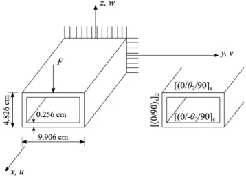
This example is concerned with the nonlinear analysis of the cantilever laminated box beam subjected to a transverse force considered by Stemple and Lee (1989); Vo and Lee (2009b); Vo and Lee (2010b); Vanegas and Patiño (2013).

The load F =1.78 kN is applied in 10 equal increments. The composite layup of each segment of the cross-section and its dimensions are shown in Figure 9. Each segment of the cross-section has eight plies, each one with a thickness of 0.032 cm. Composite layups of the webs are constant, but layups of the flange can change with θ. The material properties are presented in Table 1.

Figure 9: Geometry and composite layup of box beam.

1

E (GPa) E₂(GPa) G₁₂(GPa) ν₁₂

146.78 10.3 6.2 0.28

(16)

The beam length is 2.54 m, which was discretized with 8 and 16 TL elements. The shell finite element model in ABAQUS was built with quadratic thick-shell elements based on Reisner-Mindlin theory, with 8 nodes and reduced integration (S8R). This mesh has 7140 elements. The loading of the shell model was applied in two points on the cross-section of the free-end. A rigid device of isotropic material with 1 mm in the longitudinal direction and Young’s modulus equals to 20000 GPa was introduced in the loaded section to enforce the plane section hypothesis.

The displacements v and w and rotation of the cross-section ψ at free-end were computed for o

90

θ = and θ =45o. The results obtained with TL element and that from the literature for F = 1.78kN are presented in Table 2. It can be noted that TL solutions are more flexible than the other solutions and do not present lateral displacement v

.

Literature

o

45

θ= _θ₌₉₀o

w (cm) v (cm) ψ (rad) w (cm) v (cm) ψ (rad)

Vanegas and Patiño (2013) 58.80 0.91 0.045 59.12 0.03 0.00 Vo and Lee (2010b) 55.00 1.20 0.072 59.12 0.03 0.00 Vo and Lee (2009b) 51.30 1.00 0.065 52.90 0.01 0.00 Stemple and Lee (1989) 48.50 1.35 0.090 53.40 0.06 0.00

TL: 8 elements 61.08 0.00 0.124 61.91 0.00 0.00

TL: 16 elements 61.10 0.00 0.124 65.97 0.00 0.00

Table 2: Free-end displacement for F =1.78 kN.

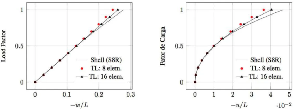
The equilibrium paths obtained using shell (S8R) and beam (TL) elements for _θ ₌₄₅o_{are depicted} in Figure 10and Table 3. It is interesting to note that the shell solution is even more flexible than TL solution. The difference is more pronounced for load factors greater than 0.7 when the shell model loses stiffness due to a local buckling near the fixed-end. It can be noted that the TL results show better agreement with the shell solution than previous results. However, it is important to note that the use of beam elements is not recommended for the load level used for this example in the literature, due to the inability of these elements to represent local buckling effects.

(17)

Load Factor Shell model TL: 16 elements

u (m) w (m) u (%) w (%)

0.1 -9.0303E-04 -6.1986E-02 -2.36 -1.44 0.2 -3.6120E-03 -1.2394E-01 -2.35 -1.41 0.3 -8.1269E-03 -1.8582E-01 -2.35 -1.37 0.4 -1.4452E-02 -2.4765E-01 -2.38 -1.32 0.5 -2.2670E-02 -3.1000E-01 -2.76 -1.46 0.6 -3.3642E-02 -3.7764E-01 -5.64 -2.93 0.7 -4.7735E-02 -4.4960E-01 -9.49* -4.88* 0.8 -6.4871E-02 -5.2346E-01 -13.01* -6.63* 0.9 -8.4938E-02 -5.9789E-01 -15.91 -8.04* 1.0 -1.0779E-01 -6.7203E-01 -18.20* -9.09*

(*) Local Buckling

Table 3: Displacements for _θ₌₄₅o _and_F ₌_{1.78 kN.}

The equilibrium paths obtained using shell (S8R) and beam (TL) elements for _θ ₌₉₀o_{are depicted} in Figure 11. The Load Control Method with automatic increment was used in the ABAQUS solution. It can be noted a very good agreement between the two solutions until a load factor about 0.6. After such load level, the beam presents local buckling, as shown in Figure 12.

Figure 11: Displacement of free-end: _θ₌₉₀0_.

(18)

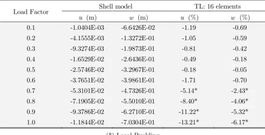
Once again, both solutions are compared in Table 4 for constant load increments. The divergence between the shell and beam results for large load factors is due to the influence of local buckling on the solution. This example shows that great care should be taken when choosing benchmark problems for comparison of finite elements for analysis of thin-walled laminated beams.

Load Factor Shell model TL: 16 elements

u (m) w (m) u (%) w (%)

0.1 -1.0404E-03 -6.6426E-02 -1.19 -0.69 0.2 -4.1555E-03 -1.3272E-01 -1.05 -0.59 0.3 -9.3274E-03 -1.9873E-01 -0.81 -0.42 0.4 -1.6529E-02 -2.6436E-01 -0.49 -0.18 0.5 -2.5746E-02 -3.2967E-01 -0.18 -0.05 0.6 -3.7651E-02 -3.9861E-01 -1.71 -0.70 0.7 -5.3101E-02 -4.7326E-01 -5.14* -2.43* 0.8 -7.1905E-02 -5.5010E-01 -8.40* -4.06* 0.9 -9.3786E-02 -6.2710E-01 -11.22* -5.32* 1.0 -1.1844E-02 -7.0304E-01 -13.21* -6.17*

(*) Local Buckling

Table 4: Displacement for _θ₌₉₀o _and_F ₌_{1.78 kN.}

4.2 Stability analysis of cantilever composite tube

This example deals with the buckling of the cantilever composite tube shown in Figure 13. The tube has mean radius R=60 mm and length L=6 m. The tube has six plies made of prepreg car-bon/epoxy AS4/3501-6, each one with thickness equal to 1 mm. Two different stacking sequences were considered: one symmetric cross-ply layup and another non-symmetric angle-ply layup, as pre-sented in Table 5

.

The material properties are given in Table 6.

Figure 13: Geometry of cantilever tube.

Models Layup

L1 [0/90/0/0/90/0]

L2 [0/90/-45/0/90/-45]

(19)

Latin American Journal of Solids and Structures 12 (2015) 2094-2117 1

E (GPa) E₂(GPa) E₃(GPa) G₁₂(GPa) G₁₃(GPa) G₂₃(GPa) ν₁₂ ν₁₃ ν₂₃

147.0 10.3 10.3 7.0 7.0 3.7 0.27 0.27 0.54

Table 6: Material properties (Daniel and Ishai, 2006).

A convergence study was carried-out for the first three buckling loads. The relative difference between shell and beam results is shown in Figure 14 for both layups. The shell model has 4816 elements (S8R). The convergence is faster for the first two buckling modes, which are bending modes with the same buckling load (Figure 15). However, it can be noted that the use of TL elements lead to very good results even for coarse meshes.

Figure 14: Convergence study.

(20)

Table 7 shows the computed results using 4816 shell elements (S8R) and 10 beam elements (TL). It can be noted that the proposed element yields very good results, for both layups, with a much lower computational cost than the use of shell elements.

Modes Shell (N) TL (N) Difference (%)

L1 L2 L1 L2 L1 L2

1 2.8322E+04 1.6530E+04 2.8443E+04 1.6538E+04 0.43 0.05 2 2.8322E+04 1.6530E+04 2.8443E+04 1.6538E+04 0.43 0.05 3 2.4763E+05 1.4728E+05 2.5600E+05 1.4886E+05 3.38 1.07

Table 7: First three buckling loads.

Finally, in order to analyze TL performance on post-buckling behavior, the tube was subjected to axial compression load F = 28.322 kN (buckling load to first and second modes) and three different values for the transverse load P (10 N, 50 N and 100 N). The equilibrium paths are shown in Figure 16. The Displacement Control method was used and a total displacement at the free-end equal to 1.2 m (w L =0.2) was applied in 50 equal increments. As expected, the transverse displacements increase with the value of the transverse load applied to the structure.

4.3 Cantilever composite tube subject to transverse load

A cantilever composite tube subject to a transverse load _P ₌₁₀_{EI L}2 _{(26.8671 kN) is considered in} this section. The equivalent bending stiffness EI was obtained using the classical expression of the Mechanics of Materials for beam displacements with the transverse displacements computed by a shell finite element model (Mororó, 2013). This example has same geometry and material properties of the previous one but now the symmetric angle-ply layup [+45/-45/+45/+45/-45/+45] is used. The tube was discretized with 8 TL elements and the obtained results were compared with a shell finite element model developed in ABAQUS. In this model, the reference load was applied at two points on the cross-section at the free-end. To avoid local effects, a rigid ring similar to the used in Example 1 was placed at the loaded section.

The equilibrium paths shown in Figure 17 were computed using the Displacement Control method by controlling the vertical displacement at the free-end until 1.8 m (w L =0.3) using 30 equal incre-ments. It can be noted that the results are in very good agreement, but when displacement increases pastw L =0.2, the difference between the solutions starts to grow. However, displacements of this magnitude are precluded by most design codes, showing that the performance of the proposed element is satisfactory for design purposes. It is important to note that no local buckling occurred in this example.

4.4 Natural frequencies of a cantilever box beam

This example presents the natural frequency analysis of a cantilever box beam with composite layup [06/456] (each ply has 1/6 mm) shown in Figure 18. The box beam has length equal to 5 m and the

(21)

Latin American Journal of Solids and Structures 12 (2015) 2094-2117 Figure 16: Transverse displacement of free-end of beam. Figure 17: Displacements of free-end of beam.

1

E (MPa) E₂(MPa) G₁₂(MPa) ν₁₂ Density (kg/m3₎

148000 9650 4550 0.3 1500

Table 8: Material properties T300/CFRP (Kollar and Pluzsik, 2002).

As in previous examples, the proposed finite element solution is compared with the results of a shell finite element model developed in ABAQUS. The shell model has 14000 elements (S8R) and 3D beam finite element model has 10 TL elements. The finite element mesh of the shell model is depicted in Figure 19.

Figure 18: Box beam cross-section. Figure 19: Detail of the mesh with shell elements (S8R) of the box beam.

(22)

Mode Shell (Hz) TL (Hz) Difference (%)

1 3.523 3.537 0.39

2 4.5167 4.530 0.30

3 21.944 22.165 1.00

Table 9: Percent difference for the first three natural frequencies.

Figure 20: Third vibration mode of the box beam (lateral bending).

5 CONCLUSIONS

This work presented a three-dimensional frame finite element for nonlinear analysis of thin-walled laminated composite beams. This element uses the Total Lagrangian formulation in order to allow the treatment of large displacements and moderate rotations.

The relation between generalized strains and stress is evaluated using a well-known theory of thin-walled beams with arbitrary layups (Kollar and Pluzsik, 2002), resulting in a fully coupled 4x4 cross-section stiffness matrix. Since the warping is neglected, this approach is particularly suited to the analysis of laminated beams with closed cross-sections.

Several numerical applications were carried-out to evaluate the performance of the proposed ele-ment. The results showed that the displacements, buckling loads and natural frequencies computed by the proposed beam element, for all considered layups, are in very good agreement with the results computed using shell elements. Therefore, this element is an excellent analysis tool for laminate com-posite beams, since it simplifies the mesh generation and leads to a much lower cost than the use of shell elements, which is the standard approach to the analysis of laminated structures with arbitrary layups.

Acknowledgements

(23)

References

Battini, J.M., (2002). Co-rotational beam elements in instability problems. Ph.D. Thesis, Royal Institute of Technology, Sweden.

Battini, J.M., Pacoste, C., (2002). Co-rotational beam elements with warping effects in stability problems. Computer Methods in Applied Mechanics and Engineering 191: 1755-1789.

Bhaskar, K., Librescu, L., (1995). A geometrically non-linear theory for laminated anisotropic thin-walled beams. International Journal of Engineering Science 33: 1331-1344.

Cardoso, J.E.B., Benedito, N.M.B., Valido, A.J.J., (2009). Finite element analysis of thin-walled composite laminated beams with geometrically nonlinear behavior including warping deformation. Thin-Walled Structures 47: 1363-1372. Cesnik, C.E.S., Hodges, D.H., (1997). VABS: A new concept for composite rotor blade cross-sectional modeling. Journal of the American Helicopter Society 42: 27-38.

Cook, R., Malkus, D., Plesha, M., Witt, R.J., (2002). Concepts and applications of finite element analysis. 4th ed., John Wiley & Sons.

Crisfield, M.A., (1991). Non-linear finite element analysis of solids and structures: essentials. 1st ed., John Wiley & Sons.

Daniel, I.M., Ishai, O., (2006). Engineering mechanics of composite materials. 2nd ed., Oxford University.

Lee, J., Lee, S., (2004). Flexural-torsional behavior of thin-walled composite beams. Thin-Walled Structures 42: 1293-1305.

Jones, R.M., (1999). Mechanics of composite materials. 2nd Ed. Philadelphia: Taylor & Francis.

Kollar, L.P., Pluzsik, A., (2002). Analysis of thin-walled composite beams with arbitrary layup. Journal of Reinforced Plastic and Composites 21: 1423-1465.

MacGuire, W., Gallagher, R.H., Ziemian, R.D., (2000). Matrix Structural Analysis. 2nd Ed., John Wiley & Sons. Mororó, L.A.T., (2013). Geometric nonlinear analysis of thin-walled laminated beams. M.Sc. Thesis (in Portuguese), Federal University of Ceará, Brazil.

Omidvar, B., Ghorbanpoor, A., (1996). A nonlinear FE solution for thin-walled open-section composite beams. Journal of Structures Engineering 11: 1369-1378.

Pluzsik, A., Kollar, L.P., (2002). Effects of shear deformation and restrained warping on the displacement of composite beams. Journal of Reinforced Plastics and Composites 21: 1517-1241.

Reddy, J.N., (2004). Mechanics of laminated composite plates and shells: theory and analysis. 2nd ed, CRC Press. Salim, H.A., Davalos, J.F., (2005). Torsion of open and closed thin-walled laminated composite section. Journal of Composite Materials 39: 497-524.

Sheikh, A.H., Thomsen, O.T., (2008). An efficient beam element for analysis of laminated composite beams of thin-walled open and closed cross sections. Composite Science and Technology 68: 2273-2281.

Simulia, (2012). ABAQUS/Standard User’s Manual – version 6.21.

Stemple, A.D., Lee, S.W., (1989). A finite element model for composite beams undergoing large deflection with arbi-trary cross-section warping. International Journal of Numerical Methods in Engineering 9: 2143-2160.

Vanegas, J.D., Patiño, I.D., (2013). Linear and non-linear finite element analysis of shear-corrected composite box beams. Latin American Journal of Solids and Structures 10: 647-673.

Vo, T.P., Lee, J., (2007). Flexural-torsional behavior of thin-walled closed-section composite box beams. Engineering Structures 29: 1774-1782.

(24)

Vo, T.P., Lee, J., (2009a). Flexural-torsional behavior of thin-walled composite space frames. International Journal of Mechanical Sciences 51: 837-845.

Vo, T.P., Lee, J., (2009b). Geometrically nonlinear analysis of thin-walled composite box beams. Computers & Struc-tures 87: 837-845.

Vo, T.P., Lee, J., (2010a). Geometrically nonlinear analysis of thin-walled open-section composite beams. Computers and Structures 88: 347-356.

Vo, T.P., Lee, J., (2010b). Geometrically nonlinear analysis of thin-walled composite box beams using shear-deformable beam theory. International Journal of Mechanics Sciences 52: 65-74.

Vo, T.P., Lee, J., (2011). Geometrical nonlinear analysis of thin-walled composite beams using finite element method based on first order shear deformation theory. Archives of Applied Mechanics 81: 419-435.