Fitted HBT Radii Versus Space-Time Variances in Flow-Dominated Models
Mike Lisa1, Evan Frodermann1, and Ulrich Heinz1 1 Department of Physics, Ohio State University,
1040 Physics Research Building,
191 West Woodruff Ave, Columbus, OH 43210, USA
Received on 20 December, 2006
The inability of otherwise successful dynamical models to reproduce the “HBT radii” extracted from two-particle correlations measured at the Relativistic Heavy Ion Collider (RHIC) is known as the “RHIC HBT Puzzle”. Most comparisons between models and experiment exploit the fact that for Gaussian sources the HBT radii agree with certain combinations of the space-time widths of the source which can be directly computed from the emission function, without having to evaluate, at significant expense, the two-particle correlation func-tion. We here study the validity of this approach for realistic emission function models some of which exhibit significant deviations from simple Gaussian behaviour. By Fourier transforming the emission function we com-pute the 2-particle correlation function and fit it with a Gaussian to partially mimic the procedure used for measured correlation functions. We describe a novel algorithm to perform this Gaussian fit analytically. We find that for realistic hydrodynamic models the HBT radii extracted from this procedure agree better with the data than the values previously extracted from the space-time widths of the emission function. Although serious discrepancies between the calculated and measured HBT radii remain, we show that a more “apples-to-apples” comparison of models with data can play an important role in any eventually successful theoretical description of RHIC HBT data.
Keywords: Non-Gaussian; Flow; Hydrodynamics; Femtoscopy; Heavy ions; Pion correlations; RHIC
I. INTRODUCTION
Two-particle intensity interferometry is widely used to characterize the space-time aspects of the freeze-out config-uration in relativistic heavy ion collisions [1]. It is common to condense this information in terms of characteristic length scales of the “homogeneity regions” [2] from which particles of a given momentum originate.
In this paper we discuss the degree to which homogene-ity lengths extracted in quite different ways may be validly compared. Throughout our study, we restrict ourselves to in-terference effects between identical, non-interacting bosons, resulting from Bose-Einstein statistics. Since final state in-teractions (e.g. Coulomb effects) affect most interferometry studies, our study may be regarded (1) as a proof-of-principle example that care must be taken to perform “apples-to-apples” comparisons, and (2) as an estimate of the magnitude of the differences for two popular theoretical models.
The homogeneity length scales are extracted in experiments by assuming that the homogeneity region can be approxi-mated by a Gaussian-profile ellipsoid in configuration space, resulting in a Gaussian two-particle momentum correlation function, and performing a semi-analytic Gaussian fit to the relative momentum dependence of the measured correlation function (see e.g. [1] for details). Following common prac-tice, we will refer in the following to the size parameters ob-tained from Gaussian fits to the correlation function as “HBT radii”.
Fitting experimental data to functional forms other than Gaussian is common in studies of elementary particle colli-sions, for which Gaussian fits clearly fail. In heavy ion col-lisions, the Gaussian ansatz works relatively well, but, es-pecially with the high quality and high-statistics data sets now available at RHIC, finer, non-Gaussian structures may
be physically interesting. Instead of inventing ad-hoc func-tional forms with which to fit the correlation functions, or functionally expanding about a Gaussian fitting form [3, 4], imaging [5–7] the homogeneity region is perhaps the most promising route to explore these structures. Indeed, recent ex-perimental imaging studies [41, 42] show clear signs of non-Gaussian behaviour. In this paper we do not take up this is-sue. Instead, we note that most experimental studies in heavy-ion physics to date have used the Gaussian ansatz [1], and we explore some ways in which HBT radii obtained in this way from data may be compared to model calculations.
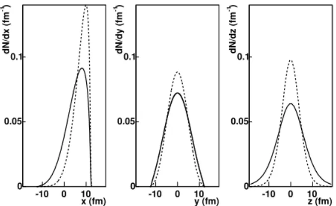
If the homogeneity region is indeed Gaussian in profile, then the HBT radii agree exactly with appropriate combina-tions of the root-mean-squared (RMS) variances of its spa-tial distribution [8]. Given a theoretical model for the freeze-out configuration, calculating these space-time variances is much easier than computing and fitting the correlation func-tion. Many comparisons between models and data therefore use this short-cut, comparing the space-time variances directly to the experimental HBT radii. However, the homogeneity re-gion is seldom perfectly Gaussian; Fig. 1 shows two-particle separation distributions from a Blast-wave model [23] which has successfully reproduced much of the data from the soft sector at RHIC.
x (fm) -10 0 10
)
-1
dN/dx (fm
0 0.05 0.1
y (fm) -10 0 10
)
-1
dN/dy (fm
0 0.05 0.1
z (fm) -10 0 10
)
-1
dN/dz (fm
0 0.05 0.1
FIG. 1: Projections of spatial freeze-out distributions (in lab frame) along the out (x), side (y), and long (z) directions, for pions withpT=
0.25 GeV/c (solid line) and 0.5 GeV/c (dashed line). From [23].
the Boltzmann/cascade approach or the shortcomings of the comparison of variances with HBT radii in the hydrody-namic case is unclear. Similarly, differences between hy-drodynamic calculations of space-time variances [9, 10] and Gaussian HBT radii fitted to three-dimensional [11–13] and one-dimensional [14, 15] correlations have been observed. However, since these calculations were performed using dif-ferent initial conditions and other parameters, it is unclear whether this, or the different extraction methods, were respon-sible for the observed differences.
Focus exclusively on the “HBT Puzzle,” per se, may be misplaced, since the transition from deconfined matter (sQGP) to confined matter is likely a crossover transition rather than a strong first-order one; in other words, there is no large latent heat associated with the transition. In this case, the large HBT radii initially predicted by models with a strong phase transition [10], are not expected after all [1]. In any event, our task here is to evaluate the degree of validity of methods of comparing model calculations to data.
Isolating the effect of the method itself is best done by using the same hydrodynamic model and parameters, and compar-ing radii calculated in different ways. One such study [16] compared space-time variances with “Gaussian radii” ex-tracted from moments of the calculated correlation function. For identical kaon correlations, the radii extracted were al-most independent of the method used. In the present study, we use a more sophisticated technique to emulate the three-dimensional Gaussian fits used by experimentalists, and we focus on pion correlations, for which the “HBT Puzzle” has been studied in detail. In our study, we find that the method used to extract the radii does, indeed, matter.
One cascade model (MPC [17]) which reports RMS vari-ances shows discrepancies with data similar to the hydrody-namic models. Studies [18–20] performed within the Boltz-mann/cascade framework show that space-time variances of the freeze-out configuration and Gaussian fits to the correla-tor can yield quite different radius parameters, mostly due to long tails in the spatial freeze-out distribution from resonance decays which strongly affect the space-time variances but are not reflected by Gaussian fits to the correlation function,
ac-cording to hydrodynamic calculations [21]. (See, however, the recent study by Kisielet al[22], which addresses this is-sue in detail in the context of a blast-wave parameterization.) Hydrodynamic calculations of the space-time variances there-fore usually do not include resonance decay contributions in the emission function [9]. Still, the comparison in [9] involves two differently determined quantities, and in the present paper we eliminate this shortcoming.
To do so requires two additional steps beyond the calcula-tion of the model emission funccalcula-tion: (i) The correlacalcula-tion func-tion must be computed via Fourier transformafunc-tion (for nonin-teracting identical particles) or by folding with a relative wave function that includes final state interaction effects (for with long-range final state interactions). This is straightforward al-beit numerically expensive since it involves multiple space-time integrals. (ii) A Gaussian fit to the three-dimensional correlation function must be performed, including a correla-tion strength parameterλas in the experiment.
We here concentrate on non-interacting pairs of identical particles as the practically most important case and also in or-der to simplify as much as possible the computation of the cor-relator. For the second step we develop an analytical Gaussian fit algorithm which reduces the multi-dimensional fit problem to a simple set of linear equations for diagonalizing a four-dimensional matrix. This should help theoretical modelers to overcome the barrier of unfamiliarity when faced with a multi-parameter fitting problem.
We apply our procedure to emission functions from hydro-dynamic calculations [9] and from the blast-wave parameter-ization [23]. Both generate non-Gaussian freeze-out distri-butions, due in large measure to finite-size effects coupled with strong collective flow which is known to be important at RHIC. On the way, we also discuss and analyze Gaussian fits to 1-dimensional projections of the 3-dimensional correla-tor. This allows for comparison with earlier work along these lines [14, 21] and first introduces our new analytic Gaussian fit algorithm in an easy and transparent simpler setting.
Much of this work has been presented previously [40].
II. VARIANCES VERSUS HBT RADII
Experimentally, the correlation function between two identical particles, as a function of their relative mo-mentum qqq≡pppa−pppb and their average (pair) momentum K
K
K≡(pppa+pppb)/2, is given by
C(qqq,KKK) =A(qqq,KKK)
B(qqq,KKK), (1) whereA(qqq,KKK)is the signal distribution andB(qqq,KKK)is the ref-erence or background distribution which is ideally similar to Ain all respects except for the presence of femtoscopic corre-lations (see e.g. [1] for details). C(qqq,KKK)is the modification to the conditional probability for measuring particleb with momentumpppb=KKK−12qqqif particleahas been measured with momentumpppa=KKK+1
the fact that the separation distribution may depend on the av-erage momentum of the pair [2] and in general does so for exploding sources [24].
Theoretically, the correlation function can be calculated from the emission functionS(ppp,x)describing the probability to emit a particle from spacetime pointxwith momentum ppp, by convoluting it with the two-particle relative wave function [1]. For pairs of non-interacting identical particles one has simply [1, 3]
C(qqq,KKK)≈1+
d4x S(KKK,x)eiq·x
d4x S(KKK,x) 2
. (2)
Here q·x=q0t −qqq·xxx, with q0=Ea−Eb=βββ·qqq where
β β
β=KKK/K0=2KKK/(Ea+Eb)is the average velocity of the pair. The≈sign in Eq. (2) indicates the “smoothness approxima-tion” which replaces bothpppaandpppbbyKKKinside the emission functions in the denominator [3]. Equation (2) can be decom-posed as
C(qqq,KKK) =1+cos(q·x)2+sin(q·x)2 (3) where. . .indicates the (KKK-dependent) space-time average with the emission function:
f ≡
d4x f(x)S(KKK,x)
d4x S(KKK,x) . (4) If S(KKK,x) is a four-dimensional Gaussian distribution of freeze-out points, the correlation function will likewise be Gaussian in the relative momentumqqq. It takes a particularly simple form for midrapidity pairs (with vanishing longitudi-nal pair momentum,KL=0) from central collisions between equal-mass spherical nuclei [1, 8]:
C(qqq) =1+λe−(q2oR2o+q2sR2s+q2lR2l). (5) Here qo,qs,ql are the relative momentum components in the Bertsch-Pratt (“out-side-long”) coordinate system [1, 8]. The pair momentum dependence of the correlation function C(qqq,KKK)leads toKKK-dependencies of the “HBT radii”Ro,Rs, andRl (which characterize the relative momentum widths of the correlation function) and of the “correlation strength”λ. For fully chaotic theoretical Gaussian sourcesλ≡1, but for experimental correlation functions usuallyλ<1. Even though we here perform a theoretical model analysis, we keepλas a parameter because Gaussian fits to non-Gaussian correlation functions generally also yieldλ=1, and experimentally such non-Gaussian effects on the extractedλ cannot be separated from other origins of reduced correlation strength (such as contamination from misidentified particles and contributions from resonance decays [1]). The HBT radii defined by Eq. (5) convey all available geometric information about the source S(KKK,x).
For Gaussian sources the radius parametersRo,Rs, andRl can be calculated directly from the source distributionS as RMS variances. For midrapidity pairs withKL=0 one finds [8]
R2o=x˜2o −2βx˜ot˜+β2t˜2,
R2s =x˜2s, R2l =x˜2l, (6)
whereβ=KT/K0is the magnitude of the (transverse) pair ve-locity (which points in thexodirection), and
˜
xµ≡xµ− xµ (7)
denotes the distance from the (KKK-dependent) center of the ho-mogeneity region for particles with momentumKKK.
Experimentalists commonly extract HBT radii by fitting their experimental correlation functions (1) with the func-tional form (5). In contrast, most (but not all) theoretical model predictions for HBT radii are based on a calculation of the space-time variances of the emission function and assum-ing the validity of Eqs. (6) which holds for Gaussian sources. Of course, there is no a priori reason to expect a source with a perfectly Gaussian profile. Even the simplest flow-dominated freeze-out parameterizations produce clear non-Gaussian tails and edges [23]. On the experimental side, high-statistics measurements show non-Gaussian behaviour, which is, however rarely treated quantitatively [4]. In the presence of such non-Gaussian features, the issues are (1) whether the two approaches yield significantly different results, and (2) whether either method characterizes the physically interesting length scales of the source sufficiently well. Here, we address the first issue in the context of blast-wave and hydrodynamic models.
Our calculations do not include experimental “noise”, par-ticle mis-identification, or contributions from the decay of long-lived resonances which can reduce the fit parameter λ in Eq. (5) from its theoretical value of unity [1, 21]. Instead, this parameter absorbs (and reflects) some of the effects of fit-ting a non-Gaussian function to a Gaussian form. This will, of course, also happen in experiment whenever the correlation function deviates from a simple Gaussian. This particular con-tribution to the fitted correlation strengthλhas so far received little attention. The model results presented here should help to assess the possible influence of non-Gaussian features in the data on the fitted values ofλ.
III. DIRECT CALCULATION OF HBT RADII
As explained in the Introduction, we here use model emis-sion functions to compute the correlation function according to Eqs. (2,3) and then fit the latter with a Gaussian, using a procedure very similar to the one used in experiment. The main difference is that the theoretical correlation function can be calculated with arbitrary precision, so the notion of a sta-tistical error does not enter. Still, we will see that the fitting problem can be formulated in a quite analogous way.
In the following subsection we introduce the algorithm for Gaussian fits through 1-dimensional cuts or projections of the dimensional correlation function. The full algorithm for 3-dimensional Gaussian fits is presented in Sec. III B.
A. One-dimensional Gaussian fits
and extracted parameters from fits toone-dimensional slices of the three-dimensional correlation function. Although those authors called them “HBT radii”, we will call them “1D radii” to distinguish them from radii extracted from full three-dimensional fits of the type performed by experimentalists.
In a given directioni(i=o,s,l) they calculate the correlator along one of the axesi:C(qi;qj=i=0). They then find the 1D
radiusR21D,iand the “directional lambda parameter”λiwhich best approximates the correlator according to
C(qi;qj=i=0)≈1+λie−q
2
iR21D,i. (8)
In particular, they calculated the correlator for a set of N valuesq(ik)(similar to experimentally binning the correlation function intoN qqq-bins) and minimized numerically the quan-tity
N
∑
k=1
ln
C(q(ik);q(jk=)i=0)−1
−lnλi+R21D,i(q
(k)
i )2
2
. (9)
This is reminiscent of the quantity typically minimized by experimenters, although in this case one also takes into ac-count the experimental uncertainty of the measured correlator by weighting each term in the sum (bin) with the inverse ex-perimental error:
χ2
1D,i≡ (10)
N
∑
k=1
lnCq(ik);q(jk=)i=0−1−lnλi+R21D,i(q
(k)
i )2
σ′(k) 1D,i
2
.
Here,σ′(k)
1D,irepresents the uncertainty in binkon the quantity to be fitted, namely lnCq(ik);q(j=k)i=0−1. It is related to the uncertaintyσ(1Dk),i on the measured correlatorC(qi(k);q(jk=)i=0) itself by
σ′1D(k),i = dlnC
q(ik);q(jk=)i=0−1 dC
qi(k);q(jk=)i=0 ·σ (k)
1D,i
= σ
(k)
1D,i C
qi(k);q(jk=)i=0
−1
. (11)
Minimization of the quantity (9) as in [21] is equivalent to setting all uncertaintiesσ′(k)
1D,i to the same constant value, in-dependent ofk. However, uncertainties on experimental cor-relation functions typically have approximately constant (k -independent) uncertainties on the bin contentsC(q(ik);q(j=k)i=0) themselves [25]. Although statistical uncertainties on cal-culated correlators may in principle be vanishingly small, the weighting factor Cq(ik);q(jk=)i=0
−12
which appears in Eq. (10) as a result of Eq. (11) will in general affect the resulting fit parameters. We choose to mimic the experi-mental situation by minimizing Eq. (10), assuming constant (i.e. k-independent) and infinitesimally small errors on C, σ(1Dk),i=σ1D,i→0.
Minimizingχ2
1D,iin Eq. (10) with respect to the fit parame-ters lnλiandR21D,iby setting
∂χ2 1D,i
∂lnλi
=0, ∂χ
2 1D,i
∂R21D,i =0, (12) we find after minimal algebra
lnλi =
X2,iY2,i−X0,iY4,i Y22,i−Y0,iY4,i
, (13)
R21D,i = X2,iY0,i−X0,iY2,i Y22,i−Y0,iY4,i
, (14)
where the quantities
Xn,i = N
∑
k=1
q(ik)n
σ′(k) 1D,i
2 lnC
qi(k);q(jk=)i=0
−1
, (15)
Yn,i = N
∑
k=1
q(ik)n
σ′(k)
1D,i
2 (16)
are directly calculable from the calculated correlator. Note that the constant errorσ1D,i of the correlator drops out from the ratios in Eqs. (13,14), so the limit σ1D,i→0 mentioned above is well-defined.
Minimization ofχ2
1D,i differs significantly from the exper-imentalists’ three-dimensional fits. In particular, it assumes complete factorization of the correlation function in theo,s,l directions. For at least two reasons, this need not be so in reality:
(i) In a full three-dimensional fit, the three directions are coupled by requiring a single λ parameter, indepen-dent of direction i. After all, according to Eq. (8) lim|qqq|→0C(qqq) =limqi→0C(qi;qj=i=0) =1+λishould be inde-pendent of direction i. Thus, allowing “directional lambda parameters” may cause the 1D fits to differ significantly from 3D fits.
(ii) Perhaps more importantly, fitting separately along the qi axes accounts for only a set of zero measure of the full three-dimensional correlation function. In particular, the cor-relation function may contain in the exponent terms such as q2oq2s orq4oq2l. (For symmetry reasons [26] odd powers ofqi vanish at midrapidity for central collisions between equal nu-clei.) Such higher order terms will affect the 3D fits of the experimentalist, but have no effect on equation (10).
We therefore now turn to full three-dimensional Gaussian fits. We will see that the above analytic expressions are easily generalized for this case.
B. Three-dimensional Gaussian fit algorithm
Proceeding as in the previous subsection, we start from the general three-dimensional Gaussian ansatz (5) which can be written as
lnC(qqq)−1=lnλ−
q2oR2o+q2sR2s+q2lR2l
If the correlation functionCqqq(k)in binkhas errorσk, the error on ln(C−1)is given as in (11) by
σ′k= σk C
q q q(k)
−1. (18)
We minimize
χ2= N
∑
k=1
lnCqqq(k)−1−lnλ+
∑
i=osl
q(ik)2R2i
σ′ k 2 (19) by setting ∂χ2 ∂lnλ =0,
∂χ2 ∂R2 i
=0 (i=o,s,l). (20)
This leads to a set of 4 coupled linear equations,
∑
βTαβPβ=Vα, (21)
whereαandβtake the values ø,o,s,l. The vectors appearing here are
P =
lnλ,R2o,R2s,R2l, (22) Vø = −
N
∑
k=1
lnCqqq(k)−1
σ′ k
2 , (23)
Vi = + N
∑
k=1
q(ik)2
σ′k2 ·ln
C
q q q(k)
−1
, (24)
while the symmetric 4×4 matrixT has components
Tøø = − N
∑
k=1 1
σ′ k
2,
Tøi = + N
∑
k=1
q(ik)2
σ′k2 , (25)
Ti j = − N
∑
k=1
q(ik)2
q(jk)2
σ′k2 .
In Equations (24) and (25)i,j=o,s,l as usual. Note the cor-respondencesVα↔Xn,iandTαβ↔Yn,i between the 3D and 1D cases.
The set of linear equations (21) is easily solved alge-braically by diagonalizing the matrixTαβ.
IV. PREVIOUS MODEL COMPARISONS
In Figs 2 and 3 are shown comparison of experimentally-measured HBT radii at RHIC to Boltzmann/cascade and hy-drodynamic models, respectively [1], for pion correlations measured at midrapidity in central collisions at RHIC. In gen-eral, the Boltzmann/cascade models do better than the hydro
(fm) out R 2 4 6
8 (fm)
side /R out R 0.5 1 1.5 2 (GeV/c) T k
0 0.5 1
(fm) side R 2 4 6 8 STAR PHENIX PHOBOS (GeV/c) T k 0.5 1 Hirano Soff Zschiesche Heinz-Kolb (fm) long R 2 4 6 8
FIG. 2: (Color online) “HBT radii” calculated [9, 15, 28, 39] in hy-drodynamic models, compared to experimental radii extracted from fits. The calculated radii are discussed in the text. Compilation from [1]. (fm) out R 2 4 6
8 (fm)
side /R out R 0.5 1 1.5 (GeV/c) T k
0 0.5 1
(fm) side R 2 4 6 8 STAR PHENIX PHOBOS (GeV/c) T k 0.5 1 (fm) long R 2 4 6 8 = 3 mb σ AMPT
= 15 mb σ AMPT = 7.73 χ MPC RQMD v2.4 HRM
FIG. 3: (Color online) “HBT radii” calculated [17, 18, 20, 38] in Boltzmann-cascade models, compared to experimental radii ex-tracted from fits. The calculated radii are discussed in the text. Com-pilation from [1].
calculations (or hybrid calculations [28] using hydro as an ini-tial stage). This may contain important information; the Equa-tion of State in Boltzmann/cascade models is generally stiffer than that used in the hydro calculations. However, the differ-ence may also come from the fact that different quantities are being compared.
None of the hydrodynamic calculations have generated HBT radii directly comparable to the data. The results for the Hirano calculation [15] are the “1D radii” R1D,i dis-cussed in Section III A. The quantities reported by Zschi-esche [39] are calculated similarly. Finally, the quantities re-ported for the Heinz and Kolb hydro [9] and the Soff hybrid hydro+cascade [28] are the spatial variances of Equation 6.
Boltz-1 1.2 1.4 1.6 1.8 2
0 0.05 0.1
qo (GeV/c) C 1D
1 1.2 1.4 1.6 1.8 2
0 0.05 0.1
qs (GeV/c) C1D
1 1.2 1.4 1.6 1.8 2
0 0.05 0.1
ql (GeV/c) C 1D
Blast-wave KT = 0 GeV/c
Correlation function
Gaussian fit
RO RS RL
λ
Variance 5.97 fm 5.97 fm 10.63 fm
HBT radius 6.13 fm 6.15 fm 9.51 fm 0.99
FIG. 4: (Color online) One-dimensional slices of the three-dimensional correlation function along the “out”, “side”, and “long” directions, for pion pairs withKKK=0, calculated from the blast-wave parameterization. For a given slice, the unplotted q-components equal 1.25 MeV/c(i.e. the center of the first bin). The solid (red) curve is the calculated correlation function from Eq. (3), the dashed (blue) curve shows the same slice of the best 3D Gaussian fit (5), with “HBT parameters” calculated from the analytic expressions given in Sec. III B.
mann/cascade calculations, labelled AMPT [20], RQMD [18], and HRM [38], full generation of a three-dimensional corre-lation function and a fit (Equation 5) to it, emulating the ex-perimental method, is performed. These represent the most apples-to-apples comparisons, and, very significantly, best de-scribe the data. It is this type of comparison which we attempt here, using the algorithm of Section III B.
V. APPLICATION TO BLAST-WAVE MODEL
Many variants of “hydrodynamically-inspired” models of freeze-out have recently been used to calculate spatial RMS variances which then were compared to experimental HBT radii. A recent example is reported in reference [23]. The model itself is very simplistic and ignores, for example, reso-nance decay contributions which may be important [21]. We ignore such issues with the model itself and simply use it here to discuss differences between RMS variances and Gaussian HBT radii.
We use “realistic” model parameters which best describe the data [4]. Specifically, we takeR=13.3 fm for the source radius, T=97 MeV for the temperature, ρ0=1.03 for the maximum transverse flow rapidity,τ=9 fm/c for the average freeze-out time, and∆τ=2.83 fm/c for the emission duration (see [23] for details).
1 1.2 1.4 1.6 1.8 2
0 0.05 0.1
qo (GeV/c) C 1D
1 1.2 1.4 1.6 1.8 2
0 0.05 0.1
qs (GeV/c) C1D
1 1.2 1.4 1.6 1.8 2
0 0.05 0.1
ql (GeV/c) C 1D
Blast-wave KT = 0.3 GeV/c
Correlation function
Gaussian fit
RO RS RL
λ
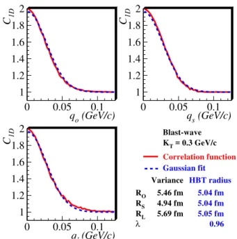
Variance 5.46 fm 4.94 fm 5.69 fm
HBT radius 5.04 fm 5.04 fm 5.05 fm 0.96
FIG. 5: (Color online) Solid (red) curves show one-dimensional slices of the three-dimensional correlation function calculated with Eq. (3) from the blast-wave parameterization, for midrapidity pions withKT=0.3 GeV/c. Dashed (blue) curves show slices of the
three-dimensional Gaussian form of Equation (5), with “HBT parameters” calculated from the analytic expressions given in Sec. III B.
3 4 5 6 7 8 9
0 0.05
out
R (fm)
0 0.05
side
0 0.05
long
q (GeV/c) 0.9
1 λo
0.9 1 λs
0.9 1
0 0.05
q (GeV/c)
λl
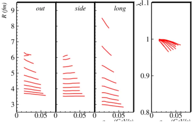
FIG. 6: (Color online) From the blast-wave parameterization, one-dimensional HBT fit parametersR1D,iandλ1D,iare calculated with
Eqs. (13,14) and plotted as a function of the maximum allowed value of anyq-component; see text for details. Each curve corresponds to one of ten values ofKT: 0.0, 0.1, 0.2, . . . , 0.9 GeV/c. Curves
corresponding to highKT are at low (high) values ofR1D,i(λ1D,i).
A. Correlation functions and analytic fits: results
Equation (12) of [23] gives the functional form for the single-pion emission function in the blast-wave model. Us-ing this forS(KKK,x), we calculate the correlation function for pion pairs with longitudinal pair momentumKL=0, using a Monte Carlo technique to numerically perform the integrals in Eq. (3).
eval-3 4 5 6 7 8 9
0 0.5
out
R (fm)
0 0.5
side
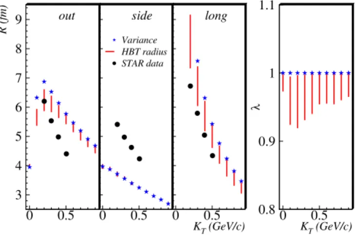
Variance HBT radius STAR data
0 0.5
long
K (GeV/c) 0.9
1 λo
0.9 1 λs
0.9 1
0 0.5
K (GeV/c)
λl
FIG. 7: (Color online) One-dimensional HBT fit parametersR1D,i
andλ1D,ias a function ofKT, calculated from the blast-wave
para-metrization with Eqs. (13,14). For a givenKT, the vertical red line
represents the variation with fit range (see Fig. 6). Blue stars rep-resent the corresponding radius parameters calculated from the RMS variances using Eq. (6). Black circles show STAR data [4], with error bars removed for clarity.
3 4 5 6 7 8 9
0 0.05
out
R (fm)
0 0.05
side
0 0.05
long
q (GeV/c) 0.8 0.9 1 1.1
0 0.05
q (GeV/c)
λ
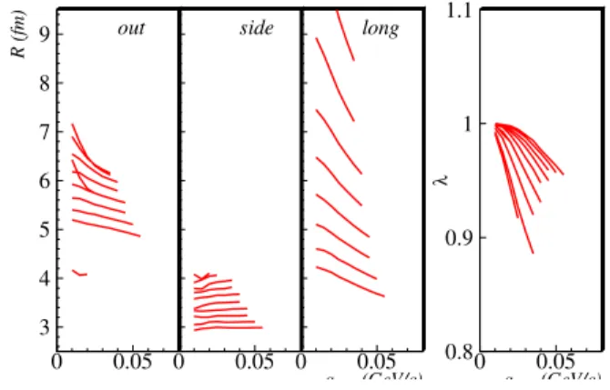
FIG. 8: (Color online) From the blast-wave parameterization, three-dimensional HBT fit parameters Ri and λ are calculated with
Eqs. (21) and plotted as a function of the maximum allowed value of anyq-component; see text for details. Each curve corresponds to one of ten values ofKT: 0.0, 0.1, 0.2, . . . , 0.9 GeV/c. Curves
corre-sponding to highKTare at low (high) values ofRi(λ). TheRlcurve
forKT=0 falls above the plotting range.
uated in finite-sized three-dimensional bins in(qo,qs,ql)of width 2.5 MeV/cin each direction. One-dimensional slices of the correlation function in the “out”, “side”, and “long” direc-tions are shown in Figs. 4 and 5, for midrapidity pion pairs withKT=0 andKT=0.3 GeV/c, respectively.
The slices of the correlation functions appear quite Gaussian, and they are tracked well by the three-dimensional Gaussian fit; the fitted correlation strengthλis very close to 1. The radius parameters calculated from the RMS variances (6) agree quite well with the HBT radii extracted from the three-dimensional Gaussian fit by solving Eqs. (21); both sets are given in the Figures. Upon closer inspection one notices, however, that the fitted outward and longitudinal radii,Roand especiallyRl, tend to be systematically smaller than those ex-tracted from the spatial RMS variances; the opposite is true
3 4 5 6 7 8 9
0 0.5
out
R (fm)
0 0.5
Variance HBT radius STAR data
side
0 0.5
long
K (GeV/c) 0.8 0.9 1 1.1
0 0.5
K (GeV/c)
λ
FIG. 9: (Color online) Three-dimensional HBT fit parametersR1D,i
andλ1D,ias a function ofKT, calculated from the blast-wave
para-metrization with Eqs. (21). For a givenKT, the vertical red line
rep-resents the variation with fit range (see Fig. 8). Blue stars represent the corresponding radius parameters calculated from the RMS vari-ances using Eq. (6). Black circles show STAR data [4], with error bars removed for clarity.
for the sideward radiiRs for which the RMS variances give slightly smaller values than the Gaussian fit. While these dif-ferences are small for the blast-wave model parameterization (at least with the “realistic” parameters studied here), they will be significantly larger (with the same basic tendencies as found here) for the hydrodynamic model source studied in Sec. VI.
The Gaussian fit parameters given in Figs. 4 and 5 corre-spond to using the largest possibleqqq-range in the sums over kin Eqs. (24,25), discarding only those data points for which Cis so close to 1 that the Monte Carlo integration sometimes yields negative values forC−1. Due to small but noticeable deviations of the correlation function from a pure Gaussian, the Gaussian fit parameters depend on the number of data points used. We study this sensitivity to the fit range in the following subsection.
B. Fit-range study
Since no measured correlation function is ever perfectly Gaussian, experimentalists typically perform so-called “fit range studies.” Here, the measured correlation function is fitted with the Gaussian form (5), using data points in a re-stricted range ofqqq. With correlation functions in the one-dimensional quantityQinv it is common to study the varia-tion of fit parameters as the first few (lowest-Qinv) data points are left out of the fit. This is because statistical fluctuations in these bins may be quite large, and due to the visible non-Gaussian nature of the measured correlation function there. Three-dimensional correlation functions do not suffer from these issues, and so usually the experimentalist includes all data points with|qi|<qmaxand studies variations of the fit pa-rameters asqmax is varied; any such variations are typically folded into systematic errors on the HBT radii.
correlation function generated from the blast-wave model, we calculate HBT parameters from 1D and 3D Gaussian fits as discussed in Sections III A and III B, restricting thek-sums in Eqs. (15), (16), (24), and (25) to include only those data points where all threeq-components have magnitudes less thanqmax [27]. Thus, we will not calculate unique HBT radii, but a finite range for each fit parameter.
For various values ofKT, Fig. 6 shows the evolution of the 1D radii withqmax. Except forRl at lowKT, the parameter variation with fit range is quite mild, corresponding to a small “non-Gaussian systematic error” on the radii. In Fig. 7 the range of this variation, indicated by vertical lines, is plotted as a function ofKT. Consistent with the theorem [8] that the spatial RMS variances (6) of the source control thecurvature of the correlatorC(qqq)atqqq=0, the blue stars in Fig. 7 coincide with theqmax→0 limit of the fitted 1D radii. The largest fit-range variations, indicating the biggest non-Gaussian effects in the correlator, are seen at small pair momentumKT. The fit-range sensitivity is most pronounced forRl (where at low KT it can exceed 0.5 fm) but almost negligible forRoandRs. In short, the 1D Gaussian fits to the two transverse projections of the correlation function give length scales consistent with the spatial RMS variances of the source distribution, but non-Gaussian features along the longitudinal projection cause the RMS variances to overestimate the longitudinal 1D HBT ra-diusRlby up to 0.5 fm at lowKT if a reasonable fit rangeqmax is used to extract the latter. This discrepancy is significantly larger than the combined statistical and systematic error on the experimental value forRl[4].
Figures 8 and 9 show the same study for the three-dimensional Gaussian fits. For reasons explained in Sec. III A, the non-Gaussian effects in a unified 3D Gaussian fit are ex-pected to differ from those in 1D fits. Indeed, in the unified 3D fit non-Gaussian influences also appear inRo, and bothRo andRlnow show fit-range variations which exceed the com-bined statistical and systematic errors of the data [4]. The largest fit-range sensitivity is still seen in the longitudinal di-rection. In Ref. [23] the blast-wave model parameters were determined by comparing RMS variances with the measured HBT radii (see Figs. 7 and 9), using the experimental errors on the latter to extract error estimates for the model parame-ters. The results presented here suggest that if the authors had instead compared the measured data with HBT radii extracted from a 3D Gaussian fit to the calculated correlation function, they would have found somewhat different model parameters whose mean values in some cases might even have fallen out-side the likely parameter range quoted in Table II of Ref. [23]. In particular, such an “apples-to-apples” comparison may al-low for somewhat larger fireball lifetimesτand/or emission durations∆τ than quoted in Ref. [23]. While such an im-proved blast-wave model fit is numerically expensive and out-side the scope of the present paper, it may be a worthwhile future project.
VI. HBT RADII FROM HYDRODYNAMICS
Non-viscous (“ideal”) hydrodynamical calculations have successfully reproduced differential momentum spectra (at
least perpendicular to the beam direction) at RHIC, including their anisotropies in non-central collisions and the dependence of these anisotropies on the masses of the emitted hadrons [9]. As in the blast-wave model calculations, very strong collective flow is a critical ingredient to reproduce the data. (Of course, in the blast-wave parameterization such flow is put in by hand while it arises naturally in the hydrodynamical model.)
Most (but not all [11–13, 15, 16]) hydrodynamic predic-tions of HBT radius parameters have been based on calcu-lations of the spatial RMS variances from the hydrodynami-cally generated emission function, using Eqs. (6) [9, 10]. In spite of the hydrodynamic model’s impressive success in de-scribing hadron spectra, these predictions of HBT radii were a failure: The calculated longitudinal radiiRl were too large (although this problem was less severe in Hirano and Tsuda’s work [15]), while the predicted sideward radiusRs was too small, and bothRsandRoshowed much less dependence on KT in theory than seen in the data. This, together with similar failures by other dynamical models (see [1] for a review), has become known as the “RHIC HBT Puzzle”.
Various possibilities to explain and correct this failure have been suggested. They include a more realistic modeling of the final freeze-out stage [28], exploration of fluctuations in the initial state and ambiguities in the hydrodynamic decoupling criterion [29], viscous effects due to incomplete thermaliza-tion (i.e. inapplicability of ideal fluid dynamics) [30], dif-ferent (more Landau-type) initial conditions leading to strong longitudinal hydrodynamic acceleration [31], and the use of more realistic or different equations of state (EoS) for the ex-panding matter [32]. None of these suggestions, individually or in combination, has been convincingly shown to be able to solve the HBT puzzle. Motivated by the blast-wave study in the preceding section, we therefore explore here one fur-ther possibility: that previous comparisons of the data with hydrodynamic models might have been misleading since the RMS variances from hydro-generated sources differ signifi-cantly from HBT radii extracted from a Gaussian parameter-ization of the correlation function. Indications that this is in-deed the case have already emerged from the work on 1D pro-jections of Hirano and Tsuda [15] and Kolb [14], and with our new analytic 3D Gaussian fit algorithm we can improve on their analysis and study this question in more detail.
and density continue to decrease. While the CE EoS was used for the hydrodynamic model predictions made for RHIC be-fore the accelerator turned on and the hadron abundances were measured, the NCE EoS is more realistic and has been used in most hydrodynamic studies since 2002. We here explore emission functions obtained with either EoS.
Figures 10-12 present 1D projections and 1D and 3D fit results, analogous to those from the previous section, for the emission function from hydrodynamic calculations using the CE EoS. Figs. 13-15 show the same for the NCE EoS. Several observations are in order.
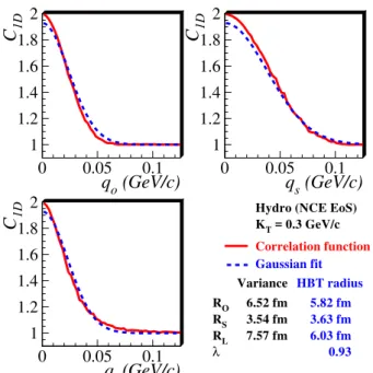
As is apparent from Figs. 10 and 13, the best 3D Gaussian fits do not fully reproduce the correlation function, even though the correlation function projections themselves appear rather Gaussian. Clearly, aspects of the correlation function not apparent in the one-dimensional projections are partially driving the 3D fit. Further, it is interesting to note that, while the projections in the “side” direction appear the worst re-produced by the fit, the greatest discrepancy between RMS variances and HBT radii are in fact in the “out” and “long” directions (c.f. Figs. 12 and 15). Both of these points empha-size that the three-dimensional correlator can contain impor-tant information which does not appear in its one-dimensional projections, and thus in the one-dimensional fits. Particularly important in this case are strong non-Gaussian features in the longitudinal direction which cause a significant suppression of the correlation strength parameterλof the 3D Gaussian fit. This in turn creates the appearance of a “bad fit” in the side-ward direction even though the 1D sideside-ward projection looks quite Gaussian itself.
One draws the same conclusion by examining the fit-range systematics. As mentioned, non-Gaussian effects generate a variation of the HBT parameters with qmax. In the three-dimensional fits (c.f. Figs. 11 and 14), the strong non-Gaussian features in theql direction now affect all four fit parameters, generating strong fit-range sensitivities also for Roandλ.
There may (and in general will) be other properties of the three-dimensional correlation function to which the 1D pro-jections and their Gaussian fits are not sensitive but which affect the 3D Gaussian fit. The extracted values forRoand Rs thus in general depend significantly on the detailed con-ditions under which the Gaussian fit is performed. Hence, a meaningful and accurate comparison between models and ex-perimental data requires that the Gaussian fit to the theoreti-cal correlation functions is done under similar conditions and constraints (e.g. fit range) as the in experiment.
VII. DISCUSSION AND CONCLUSIONS
Let us close with some general observations and summarize our conclusions.
Except inasmuch as it couples HBT radii in a 3D fit, we have not focused here on theλparameter, since comparison to measurements ofλis significantly complicated by exper-imental artifacts [1]. This is also the reason why tests of consistency between different experiments generally compare
1 1.2 1.4 1.6 1.8 2
0 0.05 0.1
q
o(GeV/c)
C
1D1 1.2 1.4 1.6 1.8 2
0 0.05 0.1
q
s(GeV/c)
C
1D1 1.2 1.4 1.6 1.8 2
0 0.05 0.1
q
l(GeV/c)
C
1DHydro (CE EoS) KT = 0.3 GeV/c
Correlation function
Gaussian fit
RO RS RL
λ
Variance
7.17 fm 3.71 fm 9.25 fm
HBT radius 6.15 fm 3.81 fm 7.21 fm 0.92
FIG. 10: (Color online) Solid (red) curves show one-dimensional slices of the three-dimensional correlation function calculated with Eq. (3) from the hydrodynamic model with CE Equation of State, for midrapidity pions withKT=0.3 GeV/c. Dashed (blue) curves show
slices of the three-dimensional Gaussian form of Equation (5), with “HBT parameters” calculated from the analytic expressions given in Sec. III B.
3 4 5 6 7 8 9
0 0.05
out
R (fm)
0 0.05
side
0 0.05
long
q (GeV/c) 0.8 0.9 1 1.1
0 0.05
q (GeV/c)
λ
FIG. 11: (Color online) From the hydrodynamic model with CE EoS, three-dimensional HBT fit parametersRiandλare calculated with
Eqs. (21) and plotted as a function of the maximum allowed value of anyq-component; see text for details. Each curve corresponds to one of ten values ofKT: 0.0, 0.1, 0.2, . . . , 0.9 GeV/c. Curves
corresponding to highKTare at low (high) values ofRi(λ). TheRl
curves forKT≤0.1 GeV/cfall above the plotting range.
HBT radii, not λ. In all of the idealized calculations pre-sented in this reportC(|qqq|=0) =2, so a purely Gaussian corre-lation function (generated by a purely Gaussian source) would yieldλ=1, with no fit-range systematics. Indeed, we find that limqmax→0λ=1 (see e.g. Fig. 11) as expected, but that its value
3 4 5 6 7 8 9
0 0.5
out
R (fm)
0 0.5
Variance HBT radius STAR data
side
0 0.5
long
K (GeV/c) 0.8 0.9 1 1.1
0 0.5
K (GeV/c)
λ
FIG. 12: (Color online) Three-dimensional HBT fit parametersR1D,i
andλ1D,i as a function of KT, calculated from the hydrodynamic
model using CE EoS with Eqs. (21). For a givenKT, the vertical
red line represents the variation with fit range (see Fig. 11). Blue stars represent the corresponding radius parameters calculated from the RMS variances using Eq. (6). Black circles show STAR data [4], with error bars removed for clarity.
1 1.2 1.4 1.6 1.8 2
0 0.05 0.1
q
o(GeV/c)
C
1D1 1.2 1.4 1.6 1.8 2
0 0.05 0.1
q
s(GeV/c)
C
1D1 1.2 1.4 1.6 1.8 2
0 0.05 0.1
q
l(GeV/c)
C
1DHydro (NCE EoS) KT = 0.3 GeV/c
Correlation function
Gaussian fit
RO RS RL
λ
Variance 6.52 fm 3.54 fm 7.57 fm
HBT radius 5.82 fm 3.63 fm 6.03 fm 0.93
FIG. 13: (Color online) Solid (red) curves show one-dimensional slices of the three-dimensional correlation function calculated with Eq. (3) from the hydrodynamic model with NCE Equation of State, for midrapidity pions withKT =0.3 GeV/c. Dashed (blue) curves
show slices of the three-dimensional Gaussian form of Equation (5), with “HBT parameters” calculated from the analytic expressions given in Sec. III B.
of unity. Our calculations confirm the generally held folklore that non-Gaussian effects may be important to understanding λ.
Of more fundamental interest are the characteristic length scales of the emission region. We have seen that RMS vari-ances of model-calculated source functions, which are fre-quently compared to experimentally extracted HBT radii, may systematically differ from “fitted” HBT radii which
character-ize the shape of the correlation function from the same model. Since the latter quantity provides the best “apples-to-apples” comparison to published experimental data, this can be an im-portant observation.
Previous attempts [14, 15, 21] to estimate the effect in hy-drodynamical calculations have focused on numerical fits to several one-dimensional projections of the calculated correla-tion funccorrela-tion. We here presented an analytic method to extract these “1D HBT radii” from the projections, and further gener-alized it to the full three-dimensional case. The 1D projections represent a set of zero measure of the full three-dimensional correlation function and, as we have seen, may not be sensitive to important three-dimensional information. This information influences the unified three-dimensional fit to the correlation function. Since the unified 3D fit most closely mimics the procedure of experimentalists, these effects are relevant for comparisons between models and data.
The magnitude of these effects are model dependent. The non-Gaussian nature of emission regions in the blast-wave pa-rameterization has been noted before [23]. It was shown here to generate only minor deviations from Gaussian behaviour in the transverse projections of the correlation function, but the longitudinal projection shows significant non-Gaussian fea-tures. In a unified 3D Gaussian fit, non-Gaussian features were seen to generate range sensitivities for all four fit-parameters, leading to significant downward shifts of bothRl andRo, especially at lowKT, relative to predictions based on the spatial RMS variances of the blast-wave source.
3 4 5 6 7 8 9
0 0.05
out
R (fm)
0 0.05
side
0 0.05
long
qmax (GeV/c)
0.8 0.9 1 1.1
0 0.05
qmax (GeV/c)
λ
FIG. 14: (Color online) From the hydrodynamic model with NCE EoS, three-dimensional HBT fit parametersRiandλare calculated
with Eqs. (21) and plotted as a function of the maximum allowed value of anyq-component; see text for details. Each curve corre-sponds to one of ten values ofKT: 0.0, 0.1, 0.2, . . . , 0.9 GeV/c.
Curves corresponding to highKTare at low (high) values ofRi(λ).
TheRlcurves forKT≤0.1 GeV/cfall above the plotting range.
3 4 5 6 7 8 9
0 0.5
out
R (fm)
0 0.5
Variance HBT radius STAR data
side
0 0.5
long
KT (GeV/c)
0.8 0.9 1 1.1
0 0.5
KT (GeV/c)
λ
FIG. 15: (Color online) Three-dimensional HBT fit parametersR1D,i
andλ1D,i as a function of KT, calculated from the hydrodynamic
model using NCE EoS with Eqs. (21). For a givenKT, the vertical
red line represents the variation with fit range (see Fig. 14). Blue stars represent the corresponding radius parameters calculated from the RMS variances using Eq. (6). Black circles show STAR data [4], with error bars removed for clarity.
In particular, for both equations of state considered here, the HBT radii in the “out” and “long” directions are significantly lower (and closer to the data) than the corresponding RMS variances which have been the basis of many “puzzle” discus-sions (c.f. Figs. 12 and 15). As in the blast-wave model, these 3D Gaussian fit effects seem to be mostly driven by strong non-Gaussian features in the longitudinal projection of the correlator. Combining improvements of using the NCE EoS and the use of HBT radii instead of RMS variances brings the hydrodynamic calculations for the longitudinal radiusRl into fair agreement with the data over the entire measuredKT range. A significant improvement is also seen in the outward direction, but it is mostly concentrated at lowKT, and hence the disagreement between the rather steepKT-dependence of the measuredRoradii and the much flatterKT-dependence of the theoretical results is getting worse. The fitted sideward radiiRsshow practically no deviation from the corresponding RMS variances, and the well-known [10] problem that the hy-drodynamically predicted values are significantly smaller and show much lessKT-dependence than the data is not alleviated by our improved comparison between theory and data.
While the results presented here cannot offer a resolution of all aspects of the “RHIC HBT Puzzle”, they refocus our
perception of where the most severe problems are located. The strong non-Gaussian effects inql direction and the re-sulting large downward shift of the fitted longitudinal radii (as compared to the corresponding RMS variances) largely eliminate the discrepancies between hydrodynamically pre-dicted and measuredRl values. A number of authors have interpreted the smallness of the measuredRl values as evi-dence for a short fireball lifetimeτf<10 fm/c, inconsistent with theO(15 fm/c)lifetimes predicted [9] by the hydrody-namic model. The analysis presented here resolves this prob-lem. On the other hand, even when using the properly ex-tracted Gaussian fit values forRsandRoand after taking into account the resulting decrease ofRoat lowKT, the theoreti-cally predicted ratioRo/Rs is still significantly larger than 1 over the entire measuredKT interval, in contradiction to the data. Furthermore, the decline of bothRoandRswith increas-ing pair momentum is still much too weak in the model, in spite of the large transverse flow generated by the hydrody-namic expansion. These aspects of the HBT Puzzle remain serious and must be addressed by other theoretical improve-ments.
Finally, one should remember that the raw experimental correlation functions hardly ever appear very Gaussian, due to additional distortions by the final state Coulomb interac-tions between the two charged particles. Modern methods of extracting the HBT radii from the measured correlator include these Coulomb effects selfconsistently in the fit function [1], leading to more complicated (numerical) fit algorithms than the analytical one presented in Section III. Nonetheless, the measured HBT radii extracted from such self-consistent 3D fits are affected by non-Gaussian structures in the underlying Bose-Einstein correlations in much the same way as discussed here for the simpler case of non-interacting particles. Thus, while Coulomb interactions should be included in future stud-ies, our analysis should provide a good estimate of the direc-tion and magnitude of non-Gaussian effects in blast-wave and hydrodynamical models, and it points out the importance of such effects in the comparison of theory to experiment.
Acknowledgments
We would like to thank the organizers of this workshop– most especially the tireless Dr. Sandra Padula– for arranging a enjoyable gathering of experts in a very productive environ-ment.
[1] M. A. Lisa, S. Pratt, R. Soltz, and U. Wiedemann, Ann. Rev. Nucl. Part. Sci.55, 357 (2005) [arXiv:nucl-ex/0505014]. [2] S. V. Akkelin and Y. M. Sinyukov, Phys. Lett. B 356, 525
(1995).
[3] U. A. Wiedemann and U. Heinz, Phys. Rev. C56, 610 (1997) [arXiv:nucl-th/9610043].
[4] J. Adamset al.[STAR Collaboration], Phys. Rev. C71, 044906 (2005) [arXiv:nucl-ex/0411036].
[5] D. A. Brown and P. Danielewicz, Phys. Lett. B398, 252 (1997)
[arXiv:nucl-th/9701010].
[6] D. A. Brown, P. Danielewicz, M. Heffner, and R. Soltz, Acta Phys. Hung. A24, 111 (2005) [arXiv:nucl-th/0404067]. [7] D. A. Brown, A. Enokizono, M. Heffner, R. Soltz,
P. Danielewicz, and S. Pratt, Phys. Rev. C72, 054902 (2005) [arXiv:nucl-th/0507015].
[8] U. A. Wiedemann and U. Heinz, Phys. Rept.319, 145 (1999) [arXiv:nucl-th/9901094].
R.C. Hwa and X.-N. Wang (World Scientific, Singapore, 2004), p. 634 [arXiv:nucl-th/0305084].
[10] U. Heinz and P. F. Kolb, inProceedings of the 18th Winter Workshop on Nuclear Dynamics, edited by R. Bellwied, J. Har-ris and W. Bauer (EP Systema, Debrecen, Hungary, 2002), p. 205 [arXiv:hep-ph/0204061].
[11] T. Hirano, K. Morita, S. Muroya, and C. Nonaka, Phys. Rev. C
65, 061902 (2002) [arXiv:nucl-th/0110009].
[12] K. Morita, S. Muroya, C. Nonaka, and T. Hirano, Phys. Rev. C
66, 054904 (2002) [arXiv:nucl-th/0205040].
[13] K. Morita and S. Muroya, Prog. Theor. Phys.111, 93 (2004) [arXiv:nucl-th/0307026].
[14] P. F. Kolb, private communication (May 2002).
[15] T. Hirano and K. Tsuda, Phys. Rev. C 66, 054905 (2002) [arXiv:nucl-th/0205043].
[16] S. Bernard, D. H. Rischke, J. A. Maruhn, and W. Greiner, Nucl. Phys. A625, 473 (1997) [arXiv:nucl-th/9703017].
[17] D. Molnar and M. Gyulassy, Phys. Rev. Lett.92, 052301 (2004) [arXiv:nucl-th/0211017].
[18] D. Hardtke and S. A. Voloshin, Phys. Rev. C61, 024905 (2000) [arXiv:nucl-th/9906033].
[19] S. Soff, S. A. Bass, D. H. Hardtke, and S. Y. Panitkin, Phys. Rev. Lett.88, 072301 (2002) [arXiv:nucl-th/0109055]. [20] Z. w. Lin, C. M. Ko, and S. Pal, Phys. Rev. Lett.89, 152301
(2002) [arXiv:nucl-th/0204054].
[21] U. A. Wiedemann and U. Heinz, Phys. Rev. C56, 3265 (1997) [arXiv:nucl-th/9611031].
[22] A. Kisiel, W. Florkowski, W. Broniowski, and J. Pluta, arXiv:nucl-th/0602039.
[23] F. Retiere and M. A. Lisa, Phys. Rev. C70, 044907 (2004) [arXiv:nucl-th/0312024].
[24] S. Pratt, Phys. Rev. Lett.53, 1219 (1984).
[25] Note that for one-dimensional correlations measured in Qinv=−qµqµ, as opposed to one-dimensional slices of the
three-dimensional correlator, phase-space considerations
usu-ally produce larger uncertainties at smallQinv.
[26] U. Heinz, A. Hummel, M. A. Lisa, and U. A. Wiedemann, Phys. Rev. C66, 044903 (2002) [arXiv:nucl-th/0207003].
[27] When the HBT radii are large (e.g. at lowKT), the correlator
approaches unity quickly with increasing|qqq|, and the quantity lnC
q q q(k)
−1
becomes numerically unwieldy; in these cases only small values ofqmaxare used.
[28] S. Soff, S. A. Bass, and A. Dumitru, Phys. Rev. Lett.86, 3981 (2001) [arXiv:nucl-th/0012085].
[29] O. J. Socolowski, F. Grassi, Y. Hama, and T. Kodama, Phys. Rev. Lett.93, 182301 (2004) [arXiv:hep-ph/0405181]. [30] D. Teaney, Phys. Rev. C68, 034913 (2003).
[31] T. Renk, Phys. Rev. C 70, 021903 (2004) [arXiv:hep-ph/0404140].
[32] P. Huovinen, Nucl. Phys. A 761, 296 (2005) [arXiv:nucl-th/0505036].
[33] J. Sollfrank et al.Phys. Rev. C 55, 392 (1997) [arXiv:nucl-th/9607029].
[34] P. F. Kolb, J. Sollfrank, and U. Heinz, Phys. Rev. C62, 054909 (2000) [arXiv:hep-ph/0006129].
[35] P. Braun-Munzinger, D. Magestro, K. Redlich, and J. Stachel, Phys. Lett. B518, 41 (2001) [arXiv:hep-ph/0105229]. [36] P. F. Kolb and R. Rapp, Phys. Rev. C 67, 044903 (2003)
[arXiv:hep-ph/0210222].
[37] D. Teaney, arXiv:nucl-th/0204023.
[38] T.J. Humanic, Nucl. Phys. A 715, 641 (2003) [arXiv:nucl-th/0205053].
[39] D. Zschiesche, S. Schramm, H. Stocker, and W. Greiner, Phys. Rev. C65, 064902 (2002) [arXiv:nucl-th/0107037].
[40] E. Frodermann, U. Heinz, and M. A. Lisa, Phys. Rev. C73, 044908 (2006) [arXiv:nucl-th/0602023].
[41] Adler, S. S., et al (PHENIX Collaboration), arXiv:nucl-ex/0605032.
![FIG. 2: (Color online) “HBT radii” calculated [9, 15, 28, 39] in hy- hy-drodynamic models, compared to experimental radii extracted from fits](https://thumb-eu.123doks.com/thumbv2/123dok_br/18982334.457501/5.892.488.818.101.327/color-online-calculated-drodynamic-models-compared-experimental-extracted.webp)