Parametrization of Bose-Einstein Correlations and Reconstruction of the Source Function in
Hadronic Z-boson Decays using the L3 Detector
W.J. Metzger, T. Nov´ak, T. Cs¨org˝o,∗ and W. Kittel for the L3 Collaboration
Radboud University, Toernooiveld 1, 6525 ED Nijmegen, The Netherlands
Received on 1 November, 2006
Bose-Einstein correlations of pairs of identical charged pions produced in hadronic Z decays are analyzed in terms of various parametrizations. A good description is achieved using a L´evy stable distribution in conjunction with a hadronization model having highly correlated configuration and momentum space, theτ-model. Using these results, the source function is reconstructed.
Keywords: Bose-Einstein Correlations
I. INTRODUCTION
In particle and nuclear physics, intensity interferometry provides a direct experimental method for the determination of sizes, shapes and lifetimes of particle-emitting sources (for reviews see [1–5]). In particular, boson interferometry pro-vides a powerful tool for the investigation of the space-time structure of particle production processes, since Bose-Einstein correlations (BEC) of two identical bosons reflect both geo-metrical and dynamical properties of the particle radiating source.
Here we study BEC in hadronic Z decay. We inves-tigate various static parametrizations in terms of the four-momentum difference,Q=−(p1−p2)2, and find that none give an adequate description of the Bose-Einstein correlation function. However, within the framework of models assum-ing strongly correlated coordinate and momentum space, a good description is achieved. We then reconstruct the com-plete space-time picture of the particle emitting source in ha-dronic Z decay.
The data used in the analysis were collected by the L3 detector [6–10] at an e+e− center-of-mass energy of √s≃ 91.2 GeV. Approximately 36 million like-sign pairs of well-measured charged tracks of about 0.8 million hadronic Z de-cays are used [11].
We perform analyses on the complete sample as well as on two- and three-jet samples. The latter are found using calorimeter clusters with the Durham jet algorithm [12–14] with a jet resolution parameterycut=0.006. To determine the thrust axis of the event we also use calorimeter clusters.
II. BOSE-EINSTEIN CORRELATION FUNCTION
The two-particle correlation function of two particles with four-momenta p1 and p2 is given by the ratio of the two-particle number density,ρ2(p1,p2), to the product of the two
∗Visitor from Budapest, Hungary, sponsored by the Scientific Exchange between Hungary (OTKA) and The Netherlands (NWO), project B64-27/N25186.
single-particle number densities, ρ1(p1)ρ1(p2). Since we are here interested only in the correlation R2 due to Bose-Einstein interference, the product of single-particle densities is replaced byρ0(p1,p2), the two-particle density that would occur in the absence of Bose-Einstein correlations:
R2(p1,p2) =
ρ2(p1,p2) ρ0(p1,p2)
. (1)
Thisρ2is corrected for detector acceptance and efficiency us-ing Monte Carlo events, to which a full detector simulation has been applied, on a bin-by-bin basis. An event mixing technique is used to constructρ0. This technique removes all correlations,e.g., resonances and energy-momentum con-servation, not just Bose-Einstein. Hence,ρ0is corrected for this [11, 15] using the JETSETMonte Carlo generator [16].
Since the mass of the two identical particles of the pair is fixed to the pion mass, the correlation function is defined in six-dimensional momentum space. Since Bose-Einstein cor-relations can be large only at small four-momentum differ-enceQ, they are often parametrized in this one-dimensional distance measure. There is no reason, however, to expect the hadron source to be spherically symmetric in jet fragmenta-tion. Recent investigations have, in fact, found an elongation of the source along the jet axis [15, 17–19]. While this effect is well established, the elongation is actually only about 20%, which suggests that a parametrization in terms of the single variableQ, may be a good approximation.
This is not the case in heavy-ion and hadron-hadron in-teractions, where BEC are found not to depend simply on Q, but on components of the momentum difference sepa-rately [5, 20–24]. However, in e+e− annihilation at lower energy [25] it has been observed that Q is the appropriate variable. We checked this and confirm that this is indeed the case: We observe [11] that R2 does not decrease when bothq2= (p1−p2)2 andq20= (E1−E2)2 are large while Q2=q2−q20is small, but is maximal forQ2=q2−q20=0, independent of the individual values ofqandq0. The same is observed in a different decomposition: Q2=Q2t +Q2L,B, whereQ2t = (pt1−pt2)
2 is the component transverse to the thrust axis andQ2L,B= (pl1−pl2)
2−(E
-0.4 -0.2 0 0.2 0.4 0.6
0 0.2 0.4 0.6 0.8 1 0.9
1 1.1 1.2 1.3 1.4
Q2
L,B Q
2 T
R2
FIG. 1:R2for two-jet events as function of the squares of the trans-verse momentum difference and the combination of longitudinal mo-mentum difference and energy difference.
observed both for two-jet and three-jet events. We conclude that a parametrization in terms ofQcan be considered a good approximation for the purposes of this article.
III. PARAMETRIZATIONS OF BEC
With a few assumptions [2, 5, 26], the two-particle corre-lation function, Eq. (1), is related to the Fourier transformed source distribution:
R2(p1,p2) =γ
1+λ|f˜(Q)|2(1+δQ), (2) where f(x)is the (configuration space) density distribution of the source, and ˜f(Q)is the Fourier transform (character-istic function) of f(x). The parameterλis introduced to ac-count for several factors, such as the possible lack of complete incoherence of particle production and the presence of long-lived resonance decays if the particle emission consists of a small, resolvable core and a halo with experimentally unre-solvable large length scales [27, 28]. The parameter γ and the (1+δQ) term parametrize possible long-range correla-tions not adequately accounted for in the reference sample. While there is no guarantee that(1+δQ)is the correct form, we will see that it does provide a good description ofR2in the regionQ>1.5 GeV.
A. Gaussian distributed source
The simplest assumption is that the source has a symmetric Gaussian distribution, in which case ˜f(Q) = expiµQ−(RQ2)2and
R2(Q) =γ1+λexp−(RQ)2(1+δQ). (3)
0.8 1 1.2 1.4 1.6 1.8 2
0 0.5 1 1.5 2 2.5 3 3.5 4
Q (GeV)
R2
(Q)
/ NDF = 234 / 96
CL = 0. %
L3 preliminary
2-jet
0.8 1 1.2 1.4 1.6 1.8 2
0 0.5 1 1.5 2 2.5 3 3.5 4
Q (GeV)
R2
(Q)
/ NDF = 132 / 95
CL = 1. %
L3 preliminary
2-jet
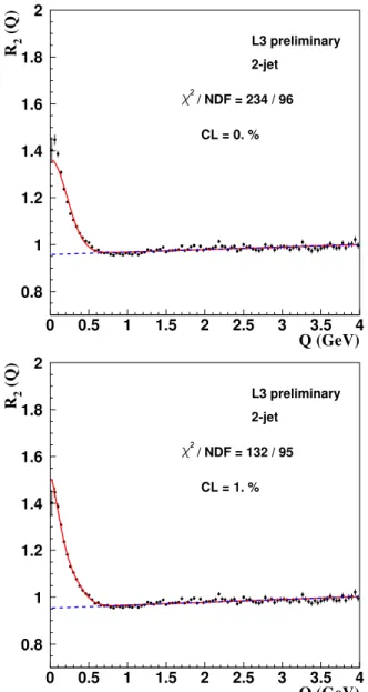
FIG. 2: (Color online) The Bose-Einstein correlation functionR2 for two-jet events with the result of a fit of (a) the Gaussian and (b) the Edgeworth parametrizations, Eqs. (3) and (4), respectively. The dashed line represents the long-range part of the fit,i.e.,γ(1+δQ).
A fit of Eq. (3) to the data results in an unacceptably low confidence level. The fit is particularly bad at lowQvalues, as is shown in Fig. 2a for two-jet events and in Fig. 3a for three-jet events, from which we conclude that the shape of the source deviates from a Gaussian.
A model-independent way to study deviations from the Gaussian parametrization is to use [5, 29, 30] the Edgeworth expansion [31] about a Gaussian. Keeping only the first non-Gaussian term, we have
R2(Q) =γ
1+λexp−(RQ)21+κ
ra-0.8 1 1.2 1.4 1.6 1.8 2
0 0.5 1 1.5 2 2.5 3 3.5 4
Q (GeV)
R2
(Q)
/ NDF = 611 / 96
CL = 0. % 3 - jet L3 preliminary
0.8 1 1.2 1.4 1.6 1.8 2
0 0.5 1 1.5 2 2.5 3 3.5 4
Q (GeV)
R2
(Q)
/ NDF = 464 / 95
CL = 0. % 3-jet
L3 preliminary
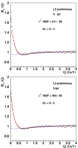
FIG. 3: (Color online) The Bose-Einstein correlation functionR2for three-jet events with the result of a fit of (a) the Gaussian and (b) the Edgeworth parametrizations, Eqs. (3) and (4), respectively. The dashed line represents the long-range part of the fit,i.e.,γ(1+δQ).
diusR.
A fit of Eq. (4) to the two-jet data, shown in Fig. 2b, is in-deed much better than the purely Gaussian fit. However, the confidence level is still marginal, and close inspection of the figure shows that the fit curve is systematically above the data in the region 0.6–1.2 GeV and that the data forQ≥1.5 GeV appear flatter than the curve, as is also the case for the purely Gaussian fit. Similar behavior is observed for three-jet events (Fig. 3b) and for all events.
B. L´evy distributed source
The symmetric L´evy stable distribution is characterized by three parameters: x0,R, andα. Its Fourier transform, ˜f(Q),
0.8 1 1.2 1.4 1.6 1.8 2
0 0.5 1 1.5 2 2.5 3 3.5 4
Q (GeV)
R2
(Q)
/ NDF = 148 / 95
CL = 0.04 %
L3 preliminary
2-jet
FIG. 4: (Color online) The Bose-Einstein correlation functionR2for two-jet events. The curve corresponds to the fit of the symmetric L´evy parametrization, Eq. (6). The dashed line represents the long-range part of the fit,i.e.,γ(1+δQ). The dot-dashed line represents a linear fit in the regionQ>1.5 GeV.
has the following form:
˜
f(Q) =exp
iQx0−| RQ|α
2
. (5)
The index of stability,α, satisfies the inequality 0<α≤2. The caseα=2 corresponds to a Gaussian source distribution with meanx0and standard deviationR. For more details, see, e.g., [32].
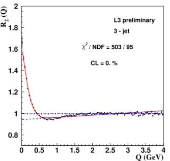
ThenR2has the following, relatively simple, form [33]: R2(Q) =γ[1+λexp(−(RQ)α)] (1+δQ). (6) From the fit of Eq. (6) to the two-jet data, shown in Fig. 4, it is clear that the correlation function is far from Gaussian: α=1.34±0.04. The confidence level, although improved compared to the fit of Eq. (3), is still unacceptably low, in fact worse than that for the Edgeworth parametrization. The same is true for three-jet events (Fig. 5) and for all events. The values ofαare 1.39±0.04 for three-jet and 1.43±0.03 for all events, respectively.
0.8 1 1.2 1.4 1.6 1.8 2
0 0.5 1 1.5 2 2.5 3 3.5 4
Q (GeV)
R2
(Q)
/ NDF = 503 / 95
CL = 0. % 3 - jet L3 preliminary
FIG. 5: (Color online) The Bose-Einstein correlation functionR2for three-jet events. The curve corresponds to the fit of the symmetric L´evy parametrization, Eq. (6). The dashed line represents the long-range part of the fit,i.e.,γ(1+δQ). The dot-dashed line represents a linear fit in the regionQ>1.5 GeV.
C. Time dependence of the source
The parametrizations discussed so far, which have proved insufficient to describe the BEC, all assume a static source. The parameterR, representing the size of the source as seen in the rest frame of the pion pair, is a constant. It has, how-ever, been observed that R depends on the transverse mass, mt=
m2+p2 t =
E2−p2
z, of the pions [34, 35]. It has been shown [36, 37] that this dependence can be understood if the produced pions satisfy, approximately, the (general-ized) Bjorken-Gottfried condition [38–43], whereby the four-momentum of a produced particle and the space-time position at which it is produced are linearly related:
xµ=dkµ. (7)
Such a correlation between space-time and momentum-energy is also a feature of the Lund string model as incor-porated in JETSET, which is very successful in describing de-tailed features of the hadronic final states of e+e− annihila-tion.
In the previous section we have seen that BEC depend, at least approximately, only onQand not on its components sep-arately. This is a non-trivial result. For a hydrodynamical type of source, on the contrary, BEC decrease when any of the rela-tive momentum components is large [5, 23]. Further, we have seen thatR2in the region 0.6–1.5 GeV dips below its values at higherQ.
A model which predicts such aQ-dependence while incor-porating the Bjorken-Gottfried condition is the so-called τ -model, described below.
1. Theτmodel
A model of strongly correlated phase-space, known as the τ-model [44], explains the experimentally found invariant rel-ative momentum dependence of Bose-Einstein correlations in e+e−reactions. This model also predicts a specific transverse mass dependence ofR2, that we subject to an experimental test here.
In this model, it is assumed that the average production point in the overall center-of-mass system,x= (t,rx,ry,rz), of particles with a given four-momentumkis given by
xµ(kµ) =dkµ. (8)
In the case of two-jet events,
d=τ/mt, (9)
wheremt is the transverse mass andτ=
t2−r2z is the lon-gitudinal proper time [60]. For isotropically distributed par-ticle production, the transverse mass is replaced by the mass in Eq. (9), while for the case of three-jet events the relation is more complicated. The second assumption is that the dis-tribution ofxµ(kµ)about its average,δ
∆(xµ(kµ)−xµ(kµ)), is narrower than the proper-time distribution. Then the emission function of theτ-model is
S(x,k) =
∞
0
dτH(τ)δ∆(x−dk)ρ1(k), (10) whereH(τ)is the longitudinal proper-time distribution, the factorδ∆(x−dk)describes the strength of the correlations be-tween coordinate space and momentum space variables and ρ1(k)is the experimentally measurable single-particle spec-trum.
The two-pion distribution,ρ2(k1,k2), is related toS(x,k), in the plane-wave approximation, by the Yano-Koonin for-mula [45]:
ρ2(k1,k2) =
d4x1d4x2S(x1,k1)S(x2,k2)
·1+cos[k1−k2] [x1−x2]. (11) Approximating the functionδ∆by a Dirac delta function, the argument of the cosine becomes
(k1−k2)(x¯1−x¯2) =−0.5(d1+d2)Q2. (12) Then the two-particle Bose-Einstein correlation function is approximated by
R2(k1,k2) =1+λReH2
Q2 2mt
, (13)
whereH(ω) = dτH(τ)exp(iωτ)is the Fourier transform of H(τ). Thus an invariant relative momentum dependent BEC appears. Note thatR2depends not only onQbut also on the average transverse mass of the two pions,mt.
choose a one-sided L´evy distribution, which has the charac-teristic function [33] (forα=1)
H(ω) =exp
−1 2
∆τ|ω|α1−isign(ω)tanαπ 2
+iωτ0
(14) where the parameterτ0is the proper time of the onset of parti-cle production and∆τis a measure of the width of the proper-time distribution. For the special caseα=1, see,e.g., [32]. Using this characteristic function in Eq. (13) yields
R2(Q,mt) = γ
1+λcos
τ0Q2 mt
+tanαπ 2
∆τQ2
2mt
α
·exp
−
∆τQ2 2mt
α
(1+δQ). (15)
2. Theτmodel for average mt
Before proceeding to fits of Eq. (15), we first consider a simplification of the equation obtained by assuming (a) that particle production starts immediately,i.e.,τ0=0, and (b) an averagemt-dependence, which is implemented in an approx-imate way by defining an effective radius,R=∆τ/(2mt). This results in:
R2(Q) =γ1+λcos(RaQ)2αexp−(RQ)2α(1+δQ), (16) whereRais related toRby
R2αa =tanαπ 2
R2α. (17)
Fits of Eq. (16) are first performed withRaas a free parameter. The fit results obtained, for two-jet, three-jet, and all events are listed in Table I and shown in Fig. 6 for two-jet events and in Fig. 7 for three-jet events. They have acceptable confidence levels, describing well the dip below unity in the 0.6–1.5 GeV region, as well as the low-Qpeak.
The fit parameters for the two-jet events satisfy Eq. (17). However, those for three-jet and all events do not. We note that the values of the parametersαandRdo not differ greatly between 2- and 3-jet samples, the most significant difference appearing to be nearly 3σforα. However, these parameters are rather highly correlated (in the fit for all events, the cor-relation coefficients areρ(λ,R) =0.95,ρ(λ,α) =−0.67 and ρ(R,α) =−0.61, which makes the simple calculation of the statistical significance of differences in the parameters unreli-able.
Fit results imposing Eq. (17) are given in Table II. For two-jet events, the values of the parameters are the same as in the fit with Ra free—only the uncertainties have changed. For three-jet and all events, the imposition of Eq. (17) results in values ofα andR closer to those for two-jet events, but the confidence levels are very bad, a consequence of incompati-bility with Eq. (17), an incompatiincompati-bility that is not surprising given that Eq. (9) is only valid for two-jet events. Therefore, we only consider two-jet events in the remaining sections of this article.
0.8 1 1.2 1.4 1.6 1.8 2
0 0.5 1 1.5 2 2.5 3 3.5 4
Q (GeV)
R2
(Q)
/ NDF = 97 / 94
CL = 40 % 2-jet
L3 preliminary
FIG. 6: (Color online) The Bose-Einstein correlation functionR2for two-jet events. The curve corresponds to the fit of the one-sided L´evy parametrization, Eq. (16). The dashed line represents the long-range part of the fit,i.e.,γ(1+δQ).
0.8 1 1.2 1.4 1.6 1.8 2
0 0.5 1 1.5 2 2.5 3 3.5 4
Q (GeV)
R2
(Q)
/ NDF = 102 / 94
CL = 27 % 3 - jet L3 preliminary
FIG. 7: (Color online) The Bose-Einstein correlation functionR2for three-jet events. The curve corresponds to the fit of the one-sided L´evy parametrization, Eq. (16). The dashed line represents the long-range part of the fit,i.e.,γ(1+δQ).
3. Theτmodel with mtdependence
TABLE I: Results of fits of Eq. (16) for two-jet, three-jet, and all events. The uncertainties are only statistical.
parameter 2-jet 3-jet all
α 0.42±0.02 0.35±0.01 0.38±0.01
λ 0.67±0.03 0.84±0.04 0.73±0.02
R(fm) 0.79±0.04 0.89±0.03 0.81±0.03
Ra(fm) 0.59±0.03 0.88±0.04 0.81±0.02 δ 0.003±0.002 –0.003±0.002 0.003±0.001 γ 0.979±0.005 1.001±0.005 0.997±0.003
χ2/DoF 97/94 102/94 98/94
confidence level 40% 27% 37%
TABLE II: Results of fits of Eq. (16) imposing Eq. (17) for two-jet, three-jet, and all events. The uncertainties are only statistical.
parameter 2-jet 3-jet all
α 0.42±0.01 0.44±0.01 0.45±0.01
λ 0.67±0.03 0.77±0.04 0.69±0.03
R(fm) 0.79±0.03 0.84±0.04 0.79±0.03 δ 0.003±0.001 0.010±0.001 0.009±0.001 γ 0.979±0.005 0.972±0.001 0.973±0.001
χ2/DoF 97/95 174/95 175/95
confidence level 42% 10−6 10−6
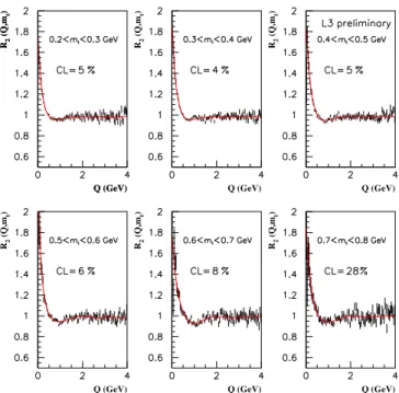
We conclude that theτ-model with a one-sided L´evy proper-time distribution describes the data with parametersτ0≈0 fm, α≈0.38±0.05 and∆τ≈3.5±0.6 fm. These values are con-sistent with the fit of Eq. (16) in the previous section, includ-ing the value ofR, which, combined with the average value of mt(0.563 GeV), corresponds to∆τ=3.5 fm. Just as in the fit of Eq. (16), the parameters of the L´evy distribution are highly correlated. Typical values of the correlation coefficients are ρ(λ,∆τ) =0.95,ρ(λ,α) =−0.67 andρ(∆τ,α) =−0.9.
IV. THE EMISSION FUNCTION OF TWO-JET EVENTS
Within the framework of theτ-model, we now reconstruct the space-time picture of the emitting process for two-jet events. The emission function in configuration space, S(x), is the proper time derivative of the integral overkof S(x,k), which in theτ-model is given by Eq. (10). Approximatingδ∆ by a Dirac delta function, we find
S(x) = d 4n dτd3r =
mt
τ
3
H(τ)ρ1
k=mtr τ
. (18)
To simplify the reconstruction ofS(x)we assume that it can be factorized in the following way:
S(r,z,t) =I(r)G(η)H(τ), (19) whereI(r)is the single-particle transverse distribution,G(η) is the space-time rapidity distribution of particle production, andH(τ) is the proper-time distribution. With the strongly correlated phase-space of theτ-model,η=yandr=ptτ/mt. Hence,
G(η) = Ny(η), (20)
I(r) = mt τ
3
Npt(rmt/τ), (21)
Q (GeV) R2
(Q,m
t
)
Q (GeV) R2
(Q,m
t
)
Q (GeV) R2
(Q,m
t
)
Q (GeV) R2
(Q,m
t
)
Q (GeV) R2
(Q,m
t
)
Q (GeV) R2
(Q,m
t
)
Q (GeV) R2
(Q,m
t
)
FIG. 8: (Color online) The results of fits of Eq. (15) to two-jet data for various intervals ofmt.
0.9 0.925 0.95 0.975 1 1.025 1.05 1.075 1.1
0 0.5 1
mT
γ
0.5 0.75 1 1.251.5 1.75 2 2.252.5
0 0.5 1
mt
λ
0 0.2 0.4 0.6 0.8 1
0 0.5 1
mt
τ0
(fm)
0 5 10 15 20 25 30 35
0 0.5 1
mt
∆τ
(fm)
0 0.1 0.2 0.3 0.4 0.5 0.6 0.7
0 0.5 1
mt
α
-0.15 -0.1 -0.05 0 0.05 0.1 0.15
0 0.5 1
mt (GeV)
δ
(GeV-1)
FIG. 9: The fit parameters from fits of Eq. (15) to two-jet data for various intervals ofmt.
whereNyandNpt are the single-particle inclusive rapidity and pt distributions, respectively. The factorization of transverse and longitudinal distributions has been checked. The distri-bution of pt is, to a good approximation, independent of the rapidity [11].
0 0.025 0.05 0.075 0.1 0.125 0.15 0.175 0.2
0 0.5 1 1.5 2 2.5 3 3.5 4
τ (fm)
H(
τ
)
FIG. 10: The proper time distribution,H(τ), forα=0.4,τ0=0 and ∆τ=3.5 fm.
-20
-10
0
10
20
z (fm)
0
10
20
t (fm)
0
1
S(z,t)
(fm ) -2
-20
-10
0
10
20
z (fm)
0
1
FIG. 11: (Color online) The temporal-longitudinal part of the source function normalized to the average number of pions per event.
with a maximum at lowt andzbut with tails reaching out to very large values oftandz, a feature also observed in hadron-hadron [46] and heavy ion collisions [47].
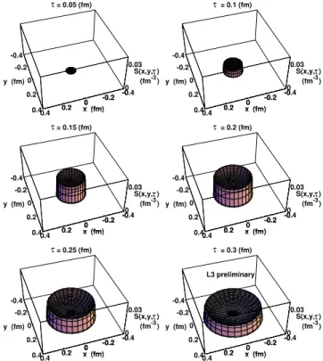
The transverse part of the emission function is obtained by integrating overzand azimuthal angle. Figure 12 shows the transverse part of the emission function for various proper times. Particle production starts immediately, increases rapidly and decreases slowly. A ring-like structure, similar to the expanding, ring-like wave created by a pebble in a pond, is observed. These pictures together form a movie that ends in about 3.5 fm, making it the shortest movie ever made of a process in nature. An animated gif file covering the first 0.3 fm (10−24sec) is available [48].
V. DISCUSSION
BEC of all events as well as two- and three-jet events are observed to be well-described by a L´evy parametrization
in-τ
= 0.05 (fm)
-0.4 -0.2 0 0.2 0.4 x (fm) -0.4
-0.2 0 0.2
0.4 y (fm)
0 0.03
τ
S(x,y, ) (fm ) -3 -0. -0.2 0 0.2 0.4 x (fm)
τ
= 0.1 (fm)
-0.4 -0.2 0 0.2 0.4 x (fm) -0.4
-0.2 0 0.2
0.4 y (fm)
0 0.03
τ
S(x,y, ) (fm ) -3 -0. -0.2 0 0.2 0.4 x (fm)
τ
= 0.15 (fm)
-0.4 -0.2 0 0.2 0.4 x (fm) -0.4
-0.2 0 0.2
0.4 y (fm)
0 0.03
τ
S(x,y, ) (fm ) -3 -0. -0.2 0 0.2 0.4 x (fm)
τ
= 0.2 (fm)
-0.4 -0.2 0 0.2 0.4 x (fm) -0.4
-0.2 0 0.2
0.4 y (fm)
0 0.03
τ
S(x,y, ) (fm ) -3 -0. -0.2 0 0.2 0.4 x (fm)
τ
= 0.25 (fm)
-0.4 -0.2 0 0.2 0.4 x (fm) -0.4
-0.2 0 0.2
0.4 y (fm)
0 0.03
τ
S(x,y, ) (fm ) -3 -0. -0.2 0 0.2 0.4 x (fm)
τ
= 0.3 (fm)
L3 preliminary
-0.4 -0.2 0 0.2 0.4 x (fm) -0.4
-0.2 0 0.2
0.4 y (fm)
0 0.03
τ
S(x,y, ) (fm ) -3 -0. -0.2 0 0.2 0.4 x (fm)
FIG. 12: (Color online) The transverse source function normalized to the average number of pions per event for various proper times.
corporating strong correlations between configuration- and momentum-space. A L´evy distribution arises naturally from a fractal, or from a random walk or anomalous diffusion [49], and the parton shower of the leading log approximation of QCD is a fractal [50–52]. In this case, the L´evy index of sta-bility is related to the strong coupling constant,αs, by[53, 54]
αs= 2π
3 α
2. (22)
Assuming (generalized) local parton hadron duality [55–57], one can expect that the distribution of hadrons retains the fea-tures of the gluon distribution. For the value ofαfound in fits of Eq. (16) we findαs=0.37±0.04 for two-jet events, This is a reasonable value for a scale of 1–2 GeV, which is where the production of hadrons takes place. For comparison, from τdecay,αs(mτ≈1.8 GeV) =0.35±0.03 [58].
It is of particular interest to point out themt dependence of the “width” of the source. In Eq. (15) the parameter as-sociated with the width is∆τ. Note that it enters Eq. (15) as ∆τQ2/mt. In a Gaussian parametrization the radiusRenters the parametrization asR2Q2. Our observance that∆τis in-dependent ofmt thus corresponds toR∝1/√mt and can be interpreted as confirmation of the observance [34, 35] of such a dependence of the Gaussian radii in 2- and 3-dimensional analyses of Z decays. The lack of dependence of all the pa-rameters of Eq. (15) on the transverse mass is in accordance with theτ-model.
and then decreases slowly, occurring predominantly close to the light cone. In the transverse plane a ring-like structure expands outwards, which is similar to the picture in
hadron-hadron interactions but unlike that of heavy ion collisions.
[1] M. Gyulassy, S.K. Kauffmann, and Lance W. Wilson, Phys. Rev. C20, 2267 (1979).
[2] David H. Boal, Claus-Konrad Gelbke, and Byron K. Jennings, Rev. Mod. Phys.62, 553 (1990).
[3] Gordon Baym, Acta Phys. Pol. B29, 1839 (1998). [4] W. Kittel, Acta Phys. Pol. C32, 3927 (2001). [5] T. Cs¨org˝o, Heavy Ion Physics15, 1 (2002).
[6] L3 Collab., B. Adevaet al., Nucl. Inst. Meth. A289, 35 (1990). [7] J.A. Bakkenet al., Nucl. Inst. Meth. A275, 81 (1989). [8] O. Adrianiet al., Nucl. Inst. Meth. A302, 53 (1991). [9] K. Deiterset al., Nucl. Inst. Meth. A323, 162 (1992). [10] M. Acciarriet al., Nucl. Inst. Meth. A351, 300 (1994). [11] Tam´as Nov´ak, Ph.D. thesis, Radboud Univ. Nijmegen, in
preparation.
[12] Yu.L. Dokshitzer, Contribution cited in Report of the Hard QCD Working Group, Proc. Workshop on Jet Studies at LEP and HERA, Durham, Dec. 1990, J. Phys. G617, 1537 (1991). [13] S. Cataniet al., Phys. Lett. B269, 432 (1991).
[14] S. Bethkeet al., Nucl. Phys. B370, 310 (1992).
[15] L3 Collab., M. Acciarriet al., Phys. Lett. B458, 517 (1999). [16] T. Sj¨ostrand, Comp. Phys. Comm.82, 74 (1994).
[17] OPAL Collab., G. Abbiendi et al., Eur. Phys. J. C16, 423 (2000).
[18] DELPHI Collab., P. Abreuet al., Phys. Lett. B471, 460 (2000). [19] ALEPH Collab., A. Heister et al., Eur. Phys. J. C 36, 147
(2004).
[20] NA22 Collab., N.M. Agababyan et al., Z. Phys. C71, 405 (1996).
[21] Ron A. Solz, Two-Pion Correlation Measurements for 14.6A·GeV/c28Si+X and 11.6A·GeV/c197Au+Au, Ph.D. the-sis, Massachusetts Inst. of Technology (1994).
[22] E-802 Collab., L. Ahleet al., Phys. Rev. C66, 054906 (2002). [23] T. Cs¨org˝o and B. L¨orstadt, Phys. Rev. C54, 1390 (1996). [24] Z. Chaje¸cki, Nucl. Phys. A774, 599 (2006).
[25] TASSO Collab., M. Althoffet al., Z. Phys. C30, 355 (1986). [26] Gerson Goldhaber, Sulamith Goldhaber, Wonyong Lee, and
Abraham Pais, Phys. Rev.120, 300 (1960). [27] J. Bolzet al., Phys. Rev. D47, 3860 (1993).
[28] T. Cs¨org˝o, B. L¨orstad, and J. Zim´anyi, Z. Phys. C 71, 491 (1996).
[29] T. Cs¨org˝o and S. Hegyi, in Proc. XXVIIIth Rencontres de Moriond, ed. ´Etienne Aug´e and J. Trˆan Thanh Vˆan, p. 635 (Edi-tions Fronti`eres, Gif-sur-Yvette, France, 1993).
[30] T. Cs¨org˝o, in Proc. Cracow Workshop on Multiparticle Produc-tion, ed. A. Białaset al., p. 175 (World Scientific, Singapore, 1994).
[31] F.Y. Edgeworth, Trans. Cambridge Phil. Soc.20, 36 (1905), see also,e.g., Harald Cram´er, Mathematical Methods of Statistics, (Princeton Univ. Press, 1946).
[32] J. P. Nolan, Stable distributions: Models for Heavy Tailed Data (2005),
http://academic2.american.edu/ ∼jpnolan/stable/CHAP1.PDF .
[33] T. Cs¨org˝o, S. Hegyi, and W.A. Zajc, Eur. Phys. J. C36, 67 (2004).
[34] B. L¨orstad and O.G. Smirnova, in Proc. 7thInt. Workshop on Multiparticle Production “Correlations and Fluctuations”, ed. R.C. Hwaet al., p. 42 (World Scientific, Singapore, 1997). [35] J.A. van Dalen, in Proc. 8th Int. Workshop on Multiparticle
Production “Correlations and Fluctuations ’98: From QCD to Particle Interferometry”, ed. T. Cs¨org˝oet al., p. 37 (World Sci-entific, Singapore, 1999).
[36] A. Białas and K. Zalewski, Acta Phys. Pol. B30, 359 (1999). [37] A. Białas, M. Kucharczyk, H. Palka, and K. Zalewski, Phys.
Rev. D62, 114007 (1999).
[38] K. Gottfried, Acta Phys. Pol. B3, 769 (1972).
[39] J.D. Bjorken, in Proc. Summer Inst. on Particle Physics, Vol. 1, p. 1 (SLAC-R-167, 1973).
[40] J.D. Bjorken, Phys. Rev. D7, 282 (1973). [41] K. Gottfried, Phys. Rev. Lett.32, 957 (1974).
[42] F.E. Low and K. Gottfried, Phys. Rev. D17, 2487 (1978). [43] J.D. Bjorken, in Proc. XXIV Int. Symp. on Multiparticle
Dy-namics, ed. A. Giovanniniet al., p. 579 (World Scientific, Sin-gapore, 1995).
[44] T. Cs¨org˝o and J. Zim´anyi, Nucl. Phys. A517, 588 (1990). [45] F.B. Yano and S.E. Koonin, Phys. Lett. B78, 556 (1978). [46] NA22 Collab., N.M. Agababyanet al., Phys. Lett. B422, 359
(1998).
[47] A. Ster, T. Cs¨org˝o, and B. L¨orstad, Nucl. Phys. A661, 419 (1999).
[48] T. Nov´ak,http://www.hef.ru.nl/ ∼novakt/movie/movie. gif.
[49] R. Metzler and J. Klafter, Phys. Rep.339, 1 (2000).
[50] P. Dahlqvist, B. Andersson, and G. Gustafson, Nucl. Phys. B 328, 76 (1989).
[51] G. Gustafson and A. Nilsson, Nucl. Phys. B355, 106 (1991). [52] G. Gustafson and A. Nilsson, Z. Phys. C52, 533 (1991). [53] T. Cs¨org˝o, S. Hegyi, T. Nov´ak, and W.A. Zajc, Acta Phys. Pol.
B36, 329 (2005).
[54] T. Cs¨org˝o, S. Hegyi, T. Nov´ak, and W.A. Zajc, Bose-Einstein or HBT correlation signature of a second order QCD phase transi-tion, 2005,http://arXiv.org/abs/nucl-th/0512060 . [55] Ya.I. Azimov, Yu.L. Dokshitzer, V.A. Khoze, and S.I. Troyan,
Z. Phys. C27, 65 (1985).
[56] Ya.I. Azimov, Yu.L. Dokshitzer, V.A. Khoze, and S.I. Troyan, Z. Phys. C31, 213 (1986).
[57] L. Van Hove and A. Giovannini, Acta Phys. Pol. B19, 931 (1988).
[58] Particle Data Group, S. Eidelmanet al., Phys. Lett. B592, 1 (2004).
[59] More correctly, dipping below the value of the parameterγ. [60] The terminology ‘longitudinal’ proper time and ‘transverse’
mass seems customary in the literature even though their
def-initions are analogousτ=
t2−r2
z andmt=