Shapes and Sizes from Non-Identical-Particle Correlations
Scott Pratt
Dept. of Physics and Astronomy, Michigan State University East Lansing, MI 48824 USA
Received on 2 December, 2006
I review the prospects for measuring source characteristics from correlations other than those involving iden-tical pions. Correlations generated from Coulomb and strong interactions are shown to provide remarkable resolving power for determining three-dimensional information, in some cases accessing more detail than can be represented by Gaussian fits.
Keywords: Correlation; Interferometry; Imaging
I. INTRODUCTION AND THEORY
As is well-known to the participants of this conference, identical-particle correlations provide insight into the space-time structure of the asymptotic phase-space density [1]. The experimentally measured two-particle correlation func-tionC(P,q)is related to the source function
S
(P,r)through a simple Fourier transform,R
P(q)≡CP(q)−1=
d3rSP(r)cos(q·r). (1) Here,P is the total momentum and q= (p1−p2)/2 is the relative momentum of the pair [2]. The source function is defined by the outgoing phase space density,
S
P(r) =
d3r1d3r2δ(r1−r2−r)f(P/2,r1,t)f(P/2,r2,t)
d3r
1d3r2f(P/2,r1,t)f(P/2,r2,t)
,
(2) where all quantities are calculated in the rest frame of the pair, whereP=0. As long as the time t is beyond any time for which particles are emitted,
S
is independent oft since both particles are moving with identical velocity, which is zero in this frame. The source function physically represents the nor-malized probability for two particles of the same velocity to be separated by a distancerin their asymptotic state. Although the source function only measures a distribution of relative distances, it still provides invaluable insight into the dynam-ics of a collision. For instance, long lived sources will lead to large separations along the direction of the pair’s velocity.Determining Sfrom the experimentally measured correla-tion funccorrela-tion in Eq. (1) is simple as one needs only Fourier transform
R
(q). Since the total momentumPis not involved in the convolution, I will suppress it in the notation for the remainder of the paper. The ability of correlations of non-identical particles to reproduce source functions is less appre-ciated by the community, despite the fact that non-identical particle correlations offer similar resolving power to identical-particle correlations in many instances [3]. Non-identical-particle correlations are driven by the strong and Coulomb interactions. After making similar, though not identical, as-sumptions as what were used for Eq. (1), the corresponding expression for the correlations are:R
(q) =d3rS(r)
|φ(q,r)|2−1. (3)
Again, the labelPis suppressed. If one views
R
(q)as a vec-tor, where each bin inqrepresents a component of the vec-tor, andS
(r) as a vector where each bin in r represents a component, determiningS from R becomes a matrix inver-sion problem, where|φ|2−1 is the matrix with labelsqandr. For the rest of the paper I will refer to the matrix as a kernel,K
(q,r) =|φ|2−1 [4].The goal of this talk is to describe the resolving power of the kernel, see [5]. In optics, “resolving power” refers to the limiting angular resolution of a lens. Here, we use the term to describe the degree to which features of the experimental correlation can be quantifiably tied to specific properties of the source. This correspondence is contained in the kernel K(q,r), which is driven by the nature of the interaction and interference between the two particles. The resolving power is of a radically different character depending on whether the particles are identical, whether they are electrically charged, or whether they interact strongly with one another.
When viewed as a matrix, the kernel
K
(q,r)is often highly singular, i.e., it may not be possible to uniquely determineS
(r)for allrfrom even perfect knowledge ofR
(q). The in-formation made accessible through the kernel depends on the unique properties of the wave function for a particular parti-cle pair. For instance, thepΛwave function is driven only by the strong interaction, which provides a large peak inR
(q) at smallq. In contrast pK+ correlations are mainly driven by the Coulomb interaction, which tends to wash out the ef-fects of the strong interaction, but provides resolving power through the Coulomb interaction itself. Before discussing the kernels I first introduce the concept of expanding the prob-lem in spherical harmonics or Cartesian harmonics in the next section. In the subsequent sections, I review the general prin-ciples determining the resolving power of the kernel for both strong and Coulomb interactions. The resolving power for ex-tracting non-Gaussian features for appsource function is then presented as an example.II. DECOMPOSING ANGULAR INFORMATION WITH
CARTESIAN OR SPHERICAL HARMONICS
harmon-ics [6]. The convenience of this decomposition derives from the fact that the specific projections of the correlations func-tion,
R
ℓ,m(q)for spherical harmonics orR
ℓx,ℓy,ℓz for Cartesianharmonics, are related to the same projection for the source function,
R
ℓm(q) = 4π
r2dr
S
ℓ,m(r)K
ℓ(q,r), (4)R
ℓ(q) = 4π
r2dr
S
ℓ(r)K
ℓ(q,r).For Cartesian harmonics,ℓ=ℓx+ℓy+ℓz. The kernel is the same for both expressions,
K
ℓ(q,r)≡12
dcosθqr
φ(q,r,cosθqr)
2
−1Pℓ(cosθqr).
(5) The projections reduce angular information for some angular functionF(Ω), which could be either
S
orR
, into a set of coefficients,FℓmorFℓ.The projections and inverses for spherical harmonics are defined as:
Fℓm ≡ (4π)−1/2
dΩF(Ω)Yℓm(Ω), (6)
F(Ω) ≡ (4π)1/2
∑
ℓ,m
FℓmYℓm(Ω).
The(2ℓ+1)complex coefficients obey the symmetryFℓm= (−1)mF∗
ℓ−m, so that the angular information for eachℓis rep-resented by(2ℓ+1)independent real numbers.
For Cartesian harmonics, the projections are defined as:
Fℓ = (2ℓ+1)!! ℓ!
dΩ
4πF(Ω)Aℓ(Ω), (7)
F(Ω) =
∑
ℓ
ℓ! ℓx!ℓy!ℓz!Fℓnˆ
ℓx
xnˆ
ℓy
ynˆℓzz
The Cartesian harmonic functionAℓ(Ω)represent products of the components of unit vectors, ˆnℓxxnˆℓyynˆℓzz , which then have lower values ofℓprojected away. Table I shows the functions forℓ≤4. Unlike the spherical harmonics, all these functions are real. For a givenℓ, there are (ℓ+1)(ℓ+2)/2 different combinations of(ℓx, ℓy, ℓz) that sum to ℓ. However, not all coefficients are independent. Since any part of the function from which one can factorn2
x+n2y+n2z =1 gives a function of lower projectionℓ, the functionsAℓand the coefficientsFℓ satisfy the “tracelessness” constraint,
Fℓx+2,ℓy,ℓz+Fℓx,ℓy+2,ℓz+Fℓx,ℓy,ℓz+2=0. (8) With this constraint, all the coefficients for a givenℓcan be generated unambiguously from knowing the(2ℓ+1) coeffi-cients forℓx=0 or 1. Thus, both expansions, with spheri-cal harmonics or Cartesian harmonics, can be represented by (2ℓ+1)real numbers for eachℓ.
The two choices of basis functions for the projections are equivalent, and it is straight forward to convert between one set of coefficients and the other. The main advantage of Carte-sian harmonics is that it is easier to identify the coefficient with the distortion of the shape as can be seen by the expan-sions in Eq. (7).
TABLE I: Cartesian harmonics forℓ≤4. Other harmonics can be found by swapping indices on both sides of the equation, e.g.,x↔ y. For example, givenA210=n2xny−ny/5, swappingy↔zgives
A201=n2xnz−nz/5.
A100(1)=nx A111(3)=nxnynz
A200(2)=n2x−(1/3) A400(4) =n4x−(6/7)n2x+ (3/35)
A110(2)=nxny A310(4)=n3xny−(3/7)nxny
A(3003) =n3x−(3/5)nx A220(4)=n2xn2y−(1/7)n2x−(1/7)n2y+ (1/35)
A210(3)=n2
xny−(1/5)ny A
(4)
211=n2xnynz−(1/7)nynz
III. THE RESOLVING POWER OF
IDENTICAL-PARTICLE STATISTICS
The kernels for identical particles are particularly simple for bosons/fermions,
K
(q,r) = (±)cos(q·r), (9)K
ℓ(q,r) = ±(−1) ℓ/2jℓ(qr), ℓ=even
0, ℓ=odd
Inverting
R
(q)to findS
(r)involves a simple Fourier trans-form. Roughly speaking, the correlation structure of levelq reveals information about components of the source function of scaleR∼1/q. Shape characteristic are also easy to invert using the kernel for specificℓ. Since jℓ(qr)behaves as(qr)ℓ,information about the distortions of a specificℓrequire look-ing at a range ofqfor whichqRℓ. The fact that the kernel does not provide resolving power for smallris not usually a problem, since the source function
S
ℓ(r)also tends to vanish for(r/R)≪ℓ.IV. THE RESOLVING POWER OF STRONG
INTERACTIONS
First, I consider the information available by analyzing the kernel forℓ=0. For q≫1/R, whereR is a characteristic scale of the source,|φ(q,r)|2differs significantly from unity only at smallr, and the kernel can be approximated by a delta function. The correlation function is then only sensitive to the probability that the two particles haver=0, with a resolving power determined by the overall density of states which is given by the scattering phase shifts,
R
ℓ=0(q) =∆dn/dq
4πq2/[(2π)3]
S
(r=0), (10)∆dn/dq = 1
π
∑
ℓ(2ℓ+1)dδℓ
dq. (11)
The sensitivity in q is determined by the form of dδℓ/dq,
rather than by details of the shape.
by the phase shifts. Forq≪1/R, the kernel is determined solely by theℓ=0 phase shifts. As long as the range of the interaction is short compared to the source size (true for heavy ion collisions), one can then approximate the wave function by a distorted plane wave. If only theℓ=0 pieces are kept,
K
(q,r)≈
eiq·r+sin(qr+δℓ=0)
qr −
sinqr qr
2
−1 (12)
K
(q→0,r)≈−2ar+a 2r2 ,
where a is the scattering length, δℓ=0 =−qa. Thus, one can crudely state that the
R
ℓ=0(q→0)provides information about the1/r2and1/rmoments of the source function, whileR
ℓ=0(q≫1/R)provides information aboutS
ℓ=0(r→ 0). Looking atdR
ℓ=0/dq2atq=0 will provide insight into other higher moments,rℓ≥0. For higher moments the con-stant of proportionality depends on theℓ=1 phase shifts and on the next higher expansion of theℓ=0 phase shift, which is determined by the effective range.Gaussian parameterizations of
S
ℓ=0(r)involve two parame-ters, a sizeRG, and a “coherence” parameterλwhich repre-sents the normalization ofS
which can differ from unity since some of the particles might originate from effectively infinite distances due to long-lived decays. Any two pieces of infor-mation aboutS
ℓ=0(r), such as the value atr=0 and a moment, are sufficient to determine the two Gaussian parameters. As explained in the previous paragraph, the kernel can, in princi-ple, provide more information. However, the ability to extract such non-Gaussian details are constrained by the strength and form of the scattering phase shifts and by statistical and sys-tematic errors in the data.The kernel forℓ >0 allows one to determine properties of the source shape. Even though the scattering phase shifts are usually important only for a few small values ofℓ,
K
ℓ(q,r)hasstrength for allℓ. This sensitivity can be explained by pointing out that for largeqr, which is the only region one can analyze for higherℓ, one can view the problem classically. The kernel is then largely determined by the shadowing. In the largeqr limit the kernel can be determined solely from the geometry of classical trajectories,
K
(q,r)|r→∞=−1r2
−σδ(−Ωqr) +dσ
dΩ . (13)
Here, the first term represents the shadowing due to particles scattering away from the direction ˆq·rˆ=−1, while the second term represents the addition due to scattered particles. Since the delta function has contributions to allℓ, the kernel from strong interactions provides resolving power at allℓfor larger r. In practice, the power falls off at largeℓ since quantum considerations destroy
K
ℓforqrℓ.The ℓ=0 kernel shown in Eq. (10) and theℓ >0 kernel shown in Eq. (13) tend to be of similar strength for most cir-cumstances. Thus, for most interactions, it can be stated that if one has sufficient statistics to measure the size, one also has the ability to determine shape.
V. THE RESOLVING POWER OF COULOMB
INTERACTIONS
Coulomb interactions also provide leverage for determin-ing source sizes. The limitations of the Coulomb interaction derives from the inherently weak couplings which make corre-lations relatively small except at smallq. At smallq,|φ|2→0, unlessris so large as to be outside the range of the Coulomb interaction,e2/r≪q2/2µ. Thus, all pairs that are emitted within a radius,r<µe2/q2
r, whereqr is the momentum reso-lution, contribute zero to the correlation function, or equiva-lently−1 to the kernel. For most experiments the resolution is of the order of 1 MeV/cand only those pairs where at least one member originates from a weak decay are uncorrelated. Thus, the intercept of the correlation function atq=0 gives
C(q→0) = (1−fl.l.)2, (14)
where fl.l.is the fraction of particles from long-lived decays.
For largeq, one can use the classical limit of the kernel given by calculating classical Coulomb trajectories,
|φ(q,r,cosθqr)|2 → d 3q
0
d3q (15)
= 1+cosθqr−x
(1+cosθqr−x)2−x2
Θ(1+cosθqr−2x).
Here,xis the ratio of the Coulomb and final-state kinetic en-ergy,
x≡2µe 2
q2r . (16)
Sincee2=1/137 is small,xis small unlessqis quite small. This allows the kernel to be approximated as
K
(q,r)|x→0 ≈ −x
2δ(1+cos(θqr), (17)
K
ℓ(q,r)|x→0 ≈ (−1)ℓx 2.
In addition toxbeing small, this approximation also relies on the classical approximation,qr≫ℓ.
The Coulomb interaction thus provides excellent resolving power for allℓ, provided thatxis not too small for the rel-evant region qR1, which can equivalently be stated that µe2Rshould not be too small, or the source size should not be too much smaller than the Bohr radius, which is 390 fm forππ
but only 58 fm forpp. Thus, one expects reasonable resolving power forpK or heavier pairs, whereas pairs involving pions offer weak resolving power through the Coulomb force. The Coulomb interaction becomes especially useful if light nuclei can be used, as in addition to the increase in the reduced mass µ, the increased factor of charges,e2→Z
1Z2e2, bolsters the resolving power.
VI. RESOLVING POWER IN THE REAL WORLD
Although the considerations of the previous sections are useful for qualitative insight, almost all kernels are affected by more than one class of interaction, and in some cases are sig-nificantly influenced by all three (e.g.,ppcorrelations). These effects then intermingle and affect the kernel in more compli-cated ways, and can not be treated in isolation.
Imaging has become a popular term for describing the in-version of
R
(q)to determineS
(q). Particular attention has been given to the ℓ =0 components by Danielewicz and Brown by fitting to splines [7–9], where non-Gaussian aspects of source functions have been observed. The spline-fitting routines are themselves a fit to a constrained functional form, and should not be mistaken for a fully flexible accounting for all possible forms for the source function. Our goal here is to gain a better feel for the sensitivity to non-Gaussian features of the source one might attain in real-world analyses.First, I will consider the simple case ofℓ=0 sources. I pick the form
S
ℓ=0(r) =λ(1−Xfrac)e−r2/2R2G
ZG
+λXfrac
e−
r2/X2+4R4
G/X4
ZX .
(18) Here, the normalization constant ensures that each source would integrate to unity when λ=1. The four parameters in this fit are:
• λ, the “coherence factor”.
• RG, a Gaussian source size.
• X, an exponential size describing the source function at larger.
• Xfrac, the fraction of the source described by the expo-nential.
The form of the argument of the second term was chosen to force the curvature at the origin to match that of the Gaussian. The upper panel of Fig. 1 shows a ppcorrelation function calculated for the form above with the parameters: λ=0.6, RG=5 fm,X =10 fm, Xfrac=0.5. In the lower panel, the change of the correlation function is illustrated for various changes in the four parameters above. Visually, it is apparent that any one of the four changes can be pretty well approxi-mated by making linear combinations of the other three. For instance, the effects of increasing the exponential lengthXby 2 fm can be approximately reproduced by a combination of re-ducingλcombined with small changes to the remaining two parameters.
The ability of an experimental analysis to determine all four parameters in Eq. (18) depends on details of the particular in-teraction and the experimental accuracy and resolution. To more rigorously determine the degree to which parameters could be experimentally constrained, theoretical correlation functions were binned, and random errors were then added. For errors of the order of what might be expected at RHIC, it did not seem possible to uniquely determine all four parame-ters. However, extracting three parameters was usually quite robust. Since a Gaussian parameterization uses only two para-meters, our exercise demonstrates that non-Gaussian features
FIG. 1: A one-dimensional pp correlation function for the para-meters shown in Eq. (18) is displayed in the upper panel, while changes corresponding to the labeled changes of the four parame-ters are shown in the lower panel. For most experiments, only three of the four parameters would be uniquely determined.
can be extracted, but that determining both the weightXfrac and the exponential scaleX will probably be outside the res-olution of the experiments. However, if one feels confident in the scaleX, e.g., one might believe it comes principally from
ωdecays, our investigations suggest that it is quite possible to confidently determine the relative weightXfrac. Most of the pairs that were investigated appeared to accommodate three-parameter analyses.
FIG. 2: (Color online) Correlations for two relative momenta are shown as a function of the angle describing the direction ofqwith respect to thezaxis for a Gaussian source of radiusRx=Ry=4,Rz=
8 fm. The angular variations forq=55 MeV/cillustrate significant resolving power for experimentally determining shapes.
harmonics for allℓ≤3.
As a point of comparison, I present identical-pion correla-tions for the same source, (Rx=Ry=4 fm,Rz=8 fm), but without the offset of the center due to the fact that there can be no offset with identical particles. As can be seen in Fig. 4, the correlations are much larger than those seen for any of the examples from Fig. 3. The stronger resolving power derives from the simple fact that all the correlations, including those forℓ=0, are several times larger. For identical particles, there are no odd-numbered harmonics. However, as shown in Fig. 4, it should be feasible to measure harmonics to rather largeℓ.
In addition to the calculations for Gaussians shown here, I have evaluated angular projections for correlations from blast wave models. From our experience thus far I can make the following rough statements regarding the prospects for dis-cerning shapes.
• For identical pion or identical kaon correlations, many values ofℓare accessible.
• ForpKorpπcorrelations: – ℓ=1 terms are easy
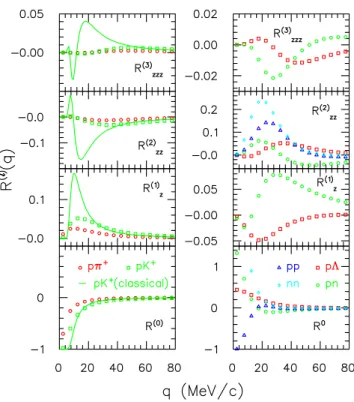
FIG. 3: (Color online) Angular projections of correlations as a func-tion ofqfor a Gaussian source of dimensionsRx=Ry=4 fm,Rz=8
fm. For non-identical particles, the center of the Gaussian was also moved by 4 fm in thezdirection. Projections are for Cartesian har-monics, withℓ=0 (lower panels),ℓx=ℓy=0, ℓz=1,2,3,
subse-quently higher panels. The solid lines forpK+describe the correla-tions one would obtain if classical trajectories were used rather than wave functions to determine the correlations weights, see Eq. (15).
FIG. 4: Angular projections of identical-pion correlations as a func-tion ofqfor a Gaussian source of dimensionsRx=Ry=4 fm,Rz=8
fm. Since the correlations are stronger for this case, larger values of ℓcan be explored.
– ℓ=2 require 1% or better accuracy – ℓ=3 are probably prohibitively small
• For baryon-baryon correlations
– ℓ=1,2 are easy
VII. SUMMARY AND PROSPECTS
Identical-pion correlations arguably represent the most dis-criminating observable at RHIC. A large fraction of the space of possible equations of state have been excluded by the-ory/experiment comparison, including strong first-order equa-tions of state, and on the opposite extreme, hard pion-gas-like equations of state. Given the paramount importance of these conclusions, it would be enormously important to verify these statements with independent analyses of space-time parame-ters using other classes of correlations. As a first goal, exper-imental analyses should work on alternative measurements of Rout/Rside/Rlong. Additionally, the odd harmonics access new features of the emission geometry. These alternative mea-surements should be viewed as being more complementary than redundant, as the theoretical basis for Coulomb-induced and strong-interaction based correlations is somewhat differ-ent from that used for iddiffer-entical-particle interference.
Exploiting other classes of shape analyses is inherently dif-ficult for two reasons. First, the strength of the correlations tends to be small. Whereas identical pion correlations are measured in the tens of percent, other classes of correlation tend to be a few percent once they are in the regionq25 MeV/c, where one can access shape information. Recent data sets from RHIC have amassed sufficient statistics to an-alyze correlation functions at the sub-one-percent level. The PHENIX experiment, with its excellent particle-identification over a wide range of momenta, is especially well poised to
exploit such correlations. STAR has even better statistics for some cases, but the delay in finishing the STAR time-of-flight wall has made it difficult to access some correlations at high statistics. For instance, since correlations are analyzed at small relative velocity (not small relative momentum)pπ cor-relations require comparing apt=100 MeV/cpion to a 700 MeV/cproton to match velocities. Both particles are at the edge of STAR’s acceptance for particle identification. How-ever, analyses will ultimately be constrained by systematic experimental errors, and from competing physical processes, such as flow or jets. All such effects must be handled more carefully when the desired correlation is of order one percent. The second challenge for analyzing these classes of cor-relation derives from the difficulty in disentangling the more complicated and opaque kernels. However, as was shown here, this is by no means insurmountable. Recently devel-oped fitting algorithms, imaging techniques, and angular de-compositions, have now been compiled into usable libraries with the CorAL (Correlations Analysis Library) project. An alpha version of the library is already available [13], and in-terested parties are encouraged to contact any of the authors, for assistance in using the codes.
Acknowledgments
The generous support of the U.S. Dept. of Energy through grant no. DE-FG02-03ER41259 is gratefully acknowledged.
[1] M. A. Lisa, S. Pratt, R. Soltz, and U. Wiedemann, Ann. Rev. Nucl. Part. Sci.55, 357 (2005) [arXiv:nucl-ex/0505014]. [2] The standard usage forππinterferometry is that the relative
mo-mentum is defined asp1−p2, which is twice what we define
asqhere. The definition in Eq. (1) is consistent with what most authors have adopted for non-identical particles.
[3] S. Pratt and S. Petriconi, Phys. Rev. C 68, 054901 (2003) [arXiv:nucl-th/0305018].
[4] It should be kept in mind that the relative wave function as-sumes non-relativistic quantum mechanics. This is valid for small relative momentum, i.e., q2/m2 ≪1, or for the case
where particles interact only through identical-particle inter-ference. Since the relevant relative momenta are typically be-low 50 MeV/c in correlation analyses, the approximation is fine for proton or kaon analyses, but might be questionable for the Coulomb interaction between pions at larger relative mo-mentum. Unfortunately, the errors associated with using non-relativistic treatments have not been studied.
[5] P. Danielewicz and S. Pratt (2006), arXiv:nucl-th/0612076, to appear in Phys. Rev.C.
[6] P. Danielewicz and S. Pratt, Phys. Lett. B 618, 60 (2005) [arXiv:nucl-th/0501003].
[7] D.A. Brown and P. Danielewicz, Phys. Rev. C 64, 014902 (2001).
[8] D.A. Brown, F. Wang and P. Danielewicz, Phys. Lett. B470, 33 (1999).
[9] D.A. Brown, P. Danielewicz, Phys. Lett. B398, 252 (1997). [10] R. Lednicky, V. L. Lyuboshits, B. Erazmus, and D. Nouais,
Phys. Lett. B373, 30 (1996).
[11] C.J. Gelderloos, et al., Phys. Rev. Lett.75, 3082 (1995). [12] S. Voloshin, R. Lednicky, S. Panitkin, and N. Xu, Phys. Rev.
Lett.79, 4766 (1997) [arXiv:nucl-th/9708044]. [13] CorALPHA web site,