Heterogeneities in Aging Models of Granular Compaction
Jeferson J. Arenzon
Instituto de Física, Universidade Federal do Rio Grande do Sul CP 15051, 91501-970 Porto Alegre RS, Brazil
Received on 4 August, 2005
Kinetically constrained models (KCM) are systems with trivial thermodynamics but often complex dynamical behavior due to constraints on the accessible paths followed by the system. Exploring these properties, the Kob-Andersen (KA) model was introduced to study the slow dynamics of glass forming liquids and later extended to granular materials. In this last context, we present new results on the heterogeneous character of both in and out of equilibrium dynamics, further stretching the granular-glass analogy.
Keywords: Granular material; Dynamical heterogeneities; Glass transition
I. INTRODUCTION
In recent years, the analogy between structural glasses and dense granular systems has become deeper and extensively explored [1–25]. As temperature is lowered, or density in-creased, respectively, both systems undergo a glass, or jam-ming, transition, where the relaxation times dramatically in-crease. Yet, in spite of all evidence of phenomenological sim-ilarity, the two systems are fundamentally different, for exam-ple, in the length scale of its components (molecules versus macroscopic particles) and the role of thermal energy (none, in the case of granulars). Because the thermal energy is too small to induce movement in these macroscopic particles, en-ergy should be externally supplied, for example, by vibrating, tapping, shearing, rotating, etc, the system, in order for a gran-ular system explore its configurational space.
Recently, the role of dynamical heterogeneities in the com-plex dynamics of glassy systems has been addressed [26–29]. The glass transition seems to be purely dynamical, with no in-creasing static correlation length as the system approaches the transition, differently from the usual critical slowing down. Thus, the increase in relaxation times seems to be related to a diverging dynamic correlation length [30–36], associ-ated to the increasing number of particles whose displace-ments become dynamically correlated, the heterogeneities, that develop during the evolution of the system. In Ref. [37] we showed, at the level of a simple, kinetically constrained model [38], that dynamical heterogeneities seem to play the same role in granular systems as they do in structural glasses, with an increasing length scale as the system approaches the jamming transition. This has also been observed in other re-cent works [20, 25, 39–41]. However, the precise role played by these structures and the associated lengths, on the dynam-ics of granular and colloidal systems, is yet to be understood. The jamming transition has also been studied in con-nection with the concept of dynamically available volume (DAV) [42, 43]. Apart from having enough nearby empty space [44], a particle is mobile if, for the particular type of model considered here, the displacement is allowed by the ki-netic constraints. Empty sites that are able to receive a neigh-boring mobile particle are calledholes. Holes can be classi-fied as either connected or not, the former being those that, by allowing a particle to jump into it may eventually
facili-tate the movements of all particles in the system. On the other hand, nonconnected holes leave a backbone of blocked parti-cles. Close to dynamical arrest, the density of connected holes decreases with the density of particles and is related with the inverse of the bootstrap length [45, 46], the average distance between two connected holes, in bootstrap percolation. In turn, this length is associated with the transport properties of the system [47–49].
Here we make an initial attempt of studying how these holes behave when the system is externally driven and falls out of equilibrium, in particular, their role during the compaction regime of granular systems, what is connected with the voids distribution measured experimentally [50]. Although we do not distinguish at this stage connected from disconnected holes, this would be important in order to fully understand the microscopic compaction mechanism.
II. KOB-ANDERSEN MODEL
The Kob-Andersen model [51] is one of the simplest mod-els describing the complex dynamics of glassy and granular systems. It consists of a lattice gas ofNparticles, each site being either empty or occupied by one particle, with no static interactions between them, i.e.,H =0. In addition, a kinetic
constraint [38] should be satisfied in order to allow the dis-placement of a particle to an empty neighboring site: there should be fewer than m occupied nearest neighbors before andafterthe move. This kinetic rule is time-reversible and detailed balance is satisfied. If the constraint is obeyed, the particle is said to be mobile and the companion vacant site is said to be a hole. At high densities, the dynamics slows down because the reduced free-volume makes it harder for a parti-cle to satisfy the dynamic constraints. These constraints were introduced to mimic the cage effect where, due to geometri-cal effects, the displacements of the particles are hindered by their neighbor particles.
dynam-ical critdynam-ical densityρc(L)<1, slowly increasing withL. At
this point, it is observed that the diffusivity falls to zero as a power law [51],D(ρ)∼(ρc−ρ)φ, withρcdepending, in
addi-tion, both on the lattice geometry and on the kinetic constraint m[37, 51, 52]. Assuming such a power law form for the diffu-sivity, finite systems, both with and without gravity, are well described, qualitatively and quantitatively, by a nonlinear dif-fusion equation [37, 53, 54].
Since much of dynamical properties of both structural glasses and dense granular materials are dictated by steric con-straints, we have generalized [22] the Kob-Andersen model by including a gravitational field. The Hamiltonian now has a one body term,βH =γ ∑izini, whereni=0,1 is the occupation
variable of thei-th site whose height iszi,γ=mg/kBT is the
inverse gravitational length andgis the constant gravitational field acting in the downward direction. We follow a contin-uous vibration dynamics, assuming that the random diffusive motion of particles, produced by the mechanical vibrations of the box, can be modeled as a thermal bath of temperature T. The particles satisfying the kinetic constraints may always move downwards while upward movements are accepted with a probabilityx=exp(−γ), related to the vibration amplitude. Particles are confined in a closed box of bcc structure, with periodic boundary conditions in the horizontal direction. We set the constraint threshold atm=5. As the Markov process generated by the kinetic rules is irreducible on the full config-uration space [22], the static properties of the model are those of a lattice-gas of non-interacting particles in a gravitational field, and these can be easily computed.
III. HETEROGENEITIES
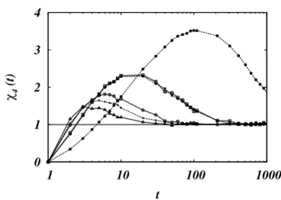
Several measures for quantifying spatial heterogeneities have been introduced for kinetic models [38]. In particular, this issue was recently investigated in the KA model [49, 55] without gravity using fourth-order correlation functions [45, 46]. In Ref. [37] these were extended to include the non-zero gravity case. In Fig. 1 we plot the dynamical nonlinear re-sponse
χ4(z,t) =N
q2(z,t)
− q(z,t)2 (1)
whereNis the number of sites in the computation,q(z,t) = C(z,t)/C(z,0)and
C(z,t) = 1
N
∑
i ni(t)ni(0)−ρ(z,t)ρ(z,0). (2) For all vibrations considered, the system is in the fluid phase and is able to achieve the asymptotic state very fast. Notice that, differently from previous works, here we measure these quantities separately around each layer of the system (to im-prove the averages,iruns over all sites in thez,z−1 andz+1 layers). In other words, we are probing horizontal, micro-scopic heterogeneities, not the macromicro-scopic ones due to the in-trinsicly inhomogeneous vertical profile. Analogously to what happens in the KA model without gravity and in other glassy0 1 2 3 4
1 10 100 1000
χ4
(t)
t
FIG. 1: Dynamical response, eq. 1, as a function of time (in MCS) for different vibrations: x=0.92 (filled symbols) and 0.94 (empty sym-bols). Different symbols stand for different heights: z=5,10 and 15 (square, circle, triangle, respectively). The line is the asymptotic
χ4=1 behavior [38]. Notice in the figure the presence of two very close curves: they correspond to different vibrations and heights, but their density is the same to within numerical accuracy. From [37].
systems, the peak is shifted to higher times and gets larger as the density increases (the lower isz, the greater is the density), which is an indication of cooperative dynamics, as larger clus-ters have more difficulty to respond to a perturbation. As these measures are done for vibrations above the apparent jamming threshold, the behavior of the system should not be affected by the finite size shortcomings discussed above and one is able to obtain the true, infinite size behavior. Indeed, the growth of the peak is compatible with the known relaxation time [48],
τ∼exp exp
c 1−ρ
(3) as can be seen in Fig. 2. Analogous results can be obtained also from the peak of the Kovacs hump [56] and persistence times distribution. Interestingly,χ4only depends onzthrough
its local density,χ4(z,t) =χ4(ρ(z),t): Fig. 1 shows that two
curves corresponding to different heights and vibrations (zand x), but having almost the same density (within numerical pre-cision), coincide.
0 1 2
2 3 4
ln ln
τ
(1 - ρ)-1
FIG. 2: Position of the peak inχ4. The growth is compatible with the known relaxation time [48], Eq. 3 (dashed line).
0 0.2 0.4 0.6 0.8
0 0.2 0.4 0.6 0.8 1
ν
ρ
0.0 0.2 0.4 0.6 0.8
0 20 40 60 80
z
FIG. 3: Density of holes as a function of density forx=0.92 (trian-gle) and 0.94 (circle), along with the results for the KA model with-out gravity (line) in a bcc lattice of height 4L, withL=20. Inset: holes profile (symbols) along with the corresponding density profiles (lines). The higherxcorresponds to the flatter density profile and to the broader holes profile.
if the system is no longer homogeneous, the local density of holes in equilibrium only depends on the local density, and not on the whole profile, or on the vibration or the height. This, together with the analogous result forχ4, if general, is an
im-portant property: as some of the quantities depend only on the local density, not on the whole profile, there is further sup-port for even simpler, one dimensional models as well as local density approximations [37, 53, 54]. >From the point of view of simulation, it is a fast way to obtain, in just one simulation, the whole profile for systems without gravity.
Upon decreasing the vibration, a finite system enters in the aging regime and the density profile develops two very dis-tinct regions [54]: an almost flat plateau atρcforz<z0and a
density decreasing region (interface) forz>z0. The position
of this plateau is size dependent and slowly increases withL, similar toρc. Analogously, the hole profile also has two
cor-responding regions (see Fig. 4 and the inset): at the interface
0 0.002 0.004 0.006 0.008 0.01
0 20 40 60 80 100
ν
(z)
z 0.0
0.5 1.0
100 105
FIG. 4: Hole profile at different times (smaller time at the top). The profile is made of two clearly separated parts:i) the interface (inset) contains almost all holes in the system and moves to the left as the system becomes compact;ii) the bulk has a much smaller hole frac-tion, that increases linearly with height. Separating these regions we have a few layers nearz=100 that are almost hole-free. The de-clivity slowly decreases with time. Notice also the difference on the vertical scales.
where most holes are localized and in the bulk, where their number is much smaller. These regions are separated by a dip with a few layers width, where there are almost no holes, corresponding to the dense layer seen in the density profile near the interface, at the top of the granular pile (this region also seems to become more localized with time), as seen in Fig. 5. At the interface, the profile is strongly peaked, and moves to the left, accompanying the interface, as the system ages (compactifies). On the other hand, in the bulk, the profile is linear, with a tangent that slowly decreases in time (although also compatible with the inverse logarithm law, a good fit is obtained witht−0.25). This evaporation of holes is the direct mechanism of the compactification process. Also, because of the almost hole-free layers between the bulk and the interface, it is very hard to exchange particles between the bulk and the interface. The interesting result here is that this process is in-homogeneous: it is faster at the topmost region of the bulk (just below the dense layer) and slower at the bottom of the system [57], as seen in Fig. 5. The oddity comes from the fact that the compaction is faster where the density is higher, the region where one would expect a slower evolution and a smaller number of holes. Instead, the evolution is faster and the number of holes is higher. Finally, it should be remarked that the small positive gradient seen in the density profile is consistent with experimental results [1, 13], although its sign is model dependent [58].
0.7 0.72 0.74 0.76 0.78 0.8
0 20 40 60 80 100
ρ
(z)
z
FIG. 5: Bulk density profile at different times (smaller time at the bottom). The region that compactifies the most is the denser one, close to the top, due to a larger number of holes.
in theνprofile, Fig. 4, contribute differently for the curve in Fig. 6: the bulk forms the highρ, small νregion near the horizontal axis (enlarged in the inset), while the interface gen-erates the rest of the curve. In the inset of Fig. 6 we can see that the bulk behavior is the opposite of what would be ex-pected at high densities: as the density increases the corre-sponding holes also increase! This explains why the density profile evolves faster near the dense layer where the density is higher: the greater the number of holes, the easier it is to com-pactify. Moreover, for different times, the curves no longer collapse (notice that the inset of Fig. 6 shows data for differ-ent times but same vibrationx). Thus, differently from the holes from the interface, there is no universal curve for the holes in the bulk. Interestingly, besides having the opposite
ρdependence, for larger times the curves move away from the equilibrium one (that is one order of magnitude above). Even the interface behavior is puzzling: layers whose density is small would be expected to be in local equilibrium. How-ever, the hole distribution only coincides with the equilibrium one forρ→0.
IV. CONCLUSIONS
In summary, besides briefly reviewing the first application of the dynamical susceptibilityχ4 in the context of granular
compaction [37], we also extended the notion of dynamically available volumes for this externally driven, out of equilib-rium situation. This is an additional similarity between struc-tural glasses and granular systems, while shedding some light on the microscopic mechanisms responsible for the slow dy-namics close to these transitions. Interestingly, the stationary behavior of the Kob-Andersen model with gravity is charac-terized by the local density, in spite of the macroscopically in-homogeneous density profile and the vibration imposed: lay-ers with the same density presents the the same time depen-dence ofχ4(z,t)as well as the same density of holes. In the
0 0.2 0.4 0.6 0.8
0 0.2 0.4 0.6 0.8 1
ν
ρ
0.000 0.005 0.010
0.74 0.75 0.76 0.77
FIG. 6: Density of holes as a function of density for several values ofxin the aging regime (0.2, circle, and 0.4, triangle), along with the equilibrium results for the KA model (line). Differently from the fluid phase, here there is no collapse of the curves onto the equilib-rium curve. Notice that there are some points withρ>ρcthat come from the oscillatory/dense layer regions. It is interesting to notice that in the case without gravity, the number of holes in the high-ρ re-gion is below the equilibrium one, while here it is above. Inset: Holes coming from the bulk forx=0.2 and three different times (from left to right:t=1072, 10974 and 99999) as a function of density. Dif-ferently from what would be expected, this an increasing function of density. In these plots we do not take into account the oscillating layers near the bottom and near the dense layer, only the bulk layers (6<z<95).
aging, compaction regime, this is no longer the case, although there is still a certain degree of universality in the behavior of the total number of holes from the interface, reflected on the collapse, at different times (but different densities), of all points onto a roughly universal curve that depends, in its turn, on the vibration (temperature). However, how connected and non-connected holes contribute to these profiles are yet to be investigated.
In addition, there are still many issues that deserve a closer inspection. Important information can also be obtained from the different sectors of theχ4(t)function [36]. However, the
range of time/density considered here is still small to resolve these different sectors. The distinction between connected and disconnected holes should also be made, as the former should be much more important in the compaction mechanism, along with the study of their spatial distribution [59]. Correlations may be also defined considering only the holes, with the asso-ciated dynamical susceptibility.
Acknowledgments
environ-ment during the last years, where part of this research was carried on.
[1] J. B. Knight, C. G. Fandrich, C. N. Lau, H. M. Jaeger, and S. R. Nagel, Phys. Rev. E51, 3957 (1995).
[2] E. R. Nowak, J. B. Knight, M. L. Povinelli, H. M. Jaeger, and S. R. Nagel, Powder Technology94, 79 (1997).
[3] A. Liu and S. Nagel, Nature396, 21 (1998).
[4] E. R. Nowak, J. B. Knight, E. Ben-Naim, , H. M. Jaeger, and S. R. Nagel, Phys. Rev. E57, 1971 (1998).
[5] J. Kurchan, inJamming and Rheology: Constrained Dynam-ics on Microscopic and Macroscopic Scales, edited by S. F. Edwards, A. Liu, and S. R. Nagel (Taylor & Francis, London, 1999), pp. 72–73, (cond-mat/9812347).
[6] C. Josserand, A. V. Tkachenko, D. M. Mueth, and H. M. Jaeger, Phys. Rev. Lett.85, 3632 (2000).
[7] M. Nicolas, P. Duru, and O. Pouliquen, Eur. Phys. J. E3, 309 (2000).
[8] A. Barrat, J. Kurchan, V. Loreto, and M. Sellitto, Phys. Rev. Lett.85, 5034 (2000).
[9] C. S. O’Hern, S. A. Langer, A. J. Liu, and S. R. Nagel, Phys. Rev. Lett.86, 111 (2001).
[10] G. D’Anna and G. Gremaud, Nature413, 407 (2001). [11] G. D’Anna and G. Gremaud, Phys. Rev. Lett. 87, 254302
(2001).
[12] L. Berthier, L. F. Cugliandolo, and J. L. Iguain, Phys. Rev. E 63, 051302 (2001).
[13] P. Philippe and D. Bideau, Europhys. Lett.60, 677 (2002). [14] L. E. Silbert, D. Ertas, G. S. Grest, T. C. Halsey, and D. Levine,
Phys. Rev. E65, 051307 (2002).
[15] H. A. Makse and J. Kurchan, Nature415, 614 (2002). [16] O. Pouliquen, M. Belzons, and M. Nicolas, Phys. Rev. Lett.91,
014301 (2003).
[17] A. Kabla and G. Debrégeas, Phys. Rev. Lett.92, 035501 (2004). [18] G. Marty and O. Dauchot, Phys. Rev. Lett.94, 015701 (2005). [19] H. Makse, J. Bruji´c, and S. Edwards, cond-mat/0503081
(un-published).
[20] O. Dauchot, G. Marty, and G. Biroli, Phys. Rev. Lett. 95, 265701 (2005).
[21] C. Song, P. Wang, and H. Makse, Proc. Nat. Acad. Sci.102, 2299 (2005).
[22] M. Sellitto and J. J. Arenzon, Phys. Rev. E62, 7793 (2000). [23] A. Coniglio and H. Herrmann, Physica A225, 1 (1995). [24] J. J. Arenzon, J. Phys. A32, L107 (1999).
[25] D. I. Goldman and H. L. Swinney, Phys. Rev. Lett.96, 145702 (2006).
[26] H. Sillescu, J. of Non-Cryst. Sol.243, 81 (1999). [27] M. D. Ediger, Annu. Rev. Phys. Chem.51, 99 (2000). [28] R. Richert, J. Phys.: Condens. Matter14, R703 (2002). [29] H. Andersen, Proc. Nat. Acad. Sci.102, 6686 (2005). [30] R. Yamamoto and A. Onuki, Phys.Rev.Lett.81, 4915 (1998).
[31] C. Bennemann, C. Donati, J. Baschnagel, and S. C. Glotzer, Nature399, 246 (1999).
[32] J. Garrahan and D. Chandler, Phys. Rev. Lett. 89, 035704 (2002).
[33] L. Berthier and J. Garrahan, J. Chem. Phys.119, 4367 (2003). [34] L. Berthier, Phys. Rev. E69, 020201(R) (2004).
[35] G. Biroli and J.-P. Bouchaud, Europhys. Lett.67, 21 (2004). [36] C. Toninelli, M. Wyart, L. Berthier, G. Biroli, and J.-P.
Bouchaud, Phys. Rev. E71, 041505 (2005).
[37] J. J. Arenzon, Y. Levin, and M. Sellitto, Physica A325, 371 (2003).
[38] F. Ritort and P. Sollich, Adv. Phys.52, 219 (2003).
[39] J. A. Drocco, M. B. Hastings, C. J. O. Reichhardt, and C. Re-ichhardt, Phys. Rev. Lett.95, 088001 (2005).
[40] A. Lefèvre, L. Berthier, and R. Stinchcombe, Phys. Rev. E72, 010301(R) (2005).
[41] L. E. Silbert, A. J. Liu, and S. R. Nagel, Phys. Rev. Lett.95, 098301 (2005).
[42] A. Mehta and G. C. Barker, J. Phys. C12, 6619 (2000). [43] A. Lawlor, D. Reagan, G. D. McCullagh, P. D. Gregorio, P.
Tartaglia, and K. Dawson, Phys. Rev. Lett.89, 245503 (2002). [44] T. Boutreux and P.-G. de Gennes, Physica A244, 59 (1997). [45] P. de Gregorio, A. Lawlor, P. Bradley, and K. Dawson, Phys.
Rev. Lett.93, 025501 (2004).
[46] P. de Gregorio, A. Lawlor, P. Bradley, and K. Dawson, Proc. Nat. Acad. Sci.102, 5669 (2005).
[47] J. Jäckle and A. Krönig, J. Phys.: Condens. Matt. 6, 7633 (1994).
[48] C. Toninelli, G. Biroli, and D. Fischer, Phys. Rev. Lett.92, 185504 (2004).
[49] C. Toninelli, G. Biroli, and D. S. Fisher, J. Stat. Phys.120, 167 (2005).
[50] P. Richard, P. Philippe, F. Barbe, S. Bourlès, X. Thibault, and D. Bideau, Phys. Rev. E68, 020301(R) (2003).
[51] K. Kob and H. Andersen, Phys. Rev. E48, 4364 (1993). [52] A. Imparato and L. Peliti, Phys. Lett. A269, 154 (2000). [53] L. Peliti and M. Sellitto, J. Phys. IV France8, Pr6 (1998). [54] Y. Levin, J. J. Arenzon, and M. Sellitto, Europhys. Lett.55, 767
(2001).
[55] S. Franz, R. Mulet, and G. Parisi, Phys. Rev. E65, 021506 (2002).
[56] J. J. Arenzon and M. Sellitto, Eur. Phys. J. B42, 543 (2004). [57] M. Sellitto, Phys. Rev. E66, 042101 (2002).
[58] P. Philippe and D. Bideau, Phys. Rev. E63, 051304 (2001). [59] A. Lawlor, P. de Gregorio, P. Bradley, M. Sellitto, and K.