Some Unusual Algebraic Structures and their
Applications in Many-Body Problems
S. S. Avancini
∗Departamento de F´ısica, Universidade Federal de Santa Catarina
Campus Trindade, C.P. 476, Florian´opolis, SC, Brazil, CEP 88.040-900
Received on 30 October, 2002
In this paper, we introduce the q-deformed and quon algebras formalism. Some applications of these alge-braic structures are considered. A possible connection of the quon algebra with composite particle systems is discussed and perspectives on using such mathematical objects in the Bose-Einstein condensation is presented.
I
Introduction
The identification of algebraic structures in quantum physi-cal systems has been an important tool for their understand-ing. Concepts of symmetry, invariance and group theory have shown to be of great utility from the beginning of quan-tum mechanics[1]. In a more recent context some unusual algebraic structures related to quantum inverse scattering methods and statistical mechanics models have appeared[2]. These algebraic structures are usually called algebras, q-deformed algebras or quantum groups. In current theoretical investigations there have been extensive applications of q-algebras to many branches of physics[3, 4, 5]. In a sense, many successful standard applications of group theory in the past may be extended to a quantum group symmetry. The aim of this paper is to discuss the use of q-algebras in the framework of many-body problems. We introduce the mathematical fundamentals as simply as possible and con-sider applications to q-deformed pseudo-spin models. These models can be considered as convenient theoretical labora-tories where one can test the properties of these algebraic structures. We also show that the q-algebra formalism may be useful in the context of boson mappings,i. e., when the substitution of fermion pairs by bosons is convenient. A q-deformed algebra has a closely related algebraic struc-ture which is called the quon algebra[6, 7]. Such algebra was proposed to describe particles that violate statistics by a small amount. We consider the applications of quon alge-bras in boson mappings and nuclear models. We also show that they may be relevant in the study of composite bosonic particles (particles composed by fermion pairs), since devi-ations of a true bosonic particle could be accommodated in a natural way through the quon algebra. This formalism can also be applied to the study of Bose-Einstein condensation in trapped atoms[8]. This paper is organized as follows: In
Sec.II quantum groups or q-algebras are defined and some of their properties and applications are analysed, in Sec.III the quon algebra formalism is considered and ,finally, in Sec.IV we present our conclusions.
II
q-deformed algebras or quantum
groups
The q-algebras or quantum groups are generalizations of classical Lie groups and Lie algebras and involve two fun-damental ideas: Deformation and Non-commutative co-multiplication[5]. Next, these two concepts will be dis-cussed in detail.
A. q-deformed objects
A q-boson algebra[9, 10] (deformed harmonic os-cillator) is a set of elements called q-boson operators:
a(annihilation), a† (creation),N (number), which sat-isfy the following commutation relations:
[N, a†] =a† , [N, a] =−a
a a†−qa†a ≡ [a, a†]
q = q−N . (1) Note that the first and second commutation relations are equal to the common harmonic oscillator, however, the third depends on the parameterqand only when q = 1we re-cover the ordinary harmonic oscillator algebra. Above, we have defined the q-commutator as
[a , a†]q ≡ a a†−q a†a . (2) This definition will be often used in this work. Although eq. (2) is valid for anyq, we consider onlyqreal orqa root
of unit, in order for the following hermitian conjugation to hold:
a† = a , N† = N .
Let us see now the consequences of the q-commutation re-lation. It follows from the q-commutation betweenaanda†
given in eq.(1) that:
a†a= (qN−q−N)/(q
−q−1) ≡[N] (3) and also:
a a†= (qN+1−q−N−1)/(q−q−1) ≡[N+ 1] , (4) where we have defined the very important object q-number or q-square brackets as:
[x]q ≡(qx−q−x)/(q−q−1) . (5) Note thatNdiffers froma†aand[x]
qgoes toxwhenqgoes to 1. It is useful to notice that the the q-boson operators can be expressed in terms of ordinary boson operators[4]. If b andb† are ordinary boson operators, where [b, b†] =
bb†−b†b= 1andN =b†b, then one can show thataand
a†can be written in terms ofbandb†through the relations:
a=b
r
[N]
N , a
† =
r
[N]
N b . (6)
The Fock space is constructed by allowing polynomials in the creation operator to act on the vacuum:
|ni = (a †)n
p
[n]! |0i a|0i= 0. (7) One can show that the action of the operators on the basis is given by
a†|ni=p[n+ 1]|n+ 1i (creation op.), a|ni=p[n]|n−1i (annihilation op.),
N|ni=n|ni (number op.). (8) We remark that these equations are very similar to the ones of the ordinary case, the only difference being the q-number appearing under the square roots instead of common num-bers.
B. q-Deformed harmonic oscillator
Analogously to the ordinary oscillator, the Hamiltonian of the q-deformed harmonic oscillator is defined as:
H= ~ω0 2 (a
†a+aa†) =~ω0
2 ([N] + [N+ 1]). (9) In this last equality, we have used the expressions foraa† anda†agiven in eqs.(3,4). Since this Hamiltonian opera-tor is diagonal in the basis|ni, the spectrum can be easily found:
H |ni=~ω0
2 ([n] + [n+ 1])|ni=En|ni. (10)
In eq.(9), we had only to substitute the operators N and
N + 1 in square brackets by the q-numbers[n]and [n+1] respectivelly.
We will show now the physical meaning of the deformation of the oscillator.
0 2 4 6 8 10 12
q=exp(0.1i) q=0.85
q=1
E
x
c
it
a
ti
on E
ner
g
y
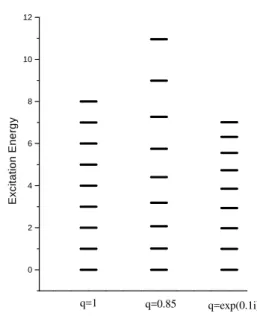
Figure 1. q-Deformed harmonic oscillator excitation energy spec-trum for 3 different values of the deformation parameterq.
In Fig.1, we can see that for the ordinary oscillator (q = 1) the spectrum is evenly spaced, however, for the deformed one (q 6= 1) the spectrum has different spacings, being uncompressed for realqand having the opposite be-havior forqa root of unity. To understand this behavior, we takeqas being equal toeτand we assume thatτis small, so up to the first order in theτparameter:q=eτ ≃ 1 +τ. Firstly substituting in the oscillator energy, eq.(10), the q numbersnandn+ 1by their explicit expressions, results in
En=
~ω0
2 ([n] + [n+ 1])
= ~ω0 2
µ
qn−q−n
q−q−1 +
qn+1−q−(n+1) q−q−1
¶
(11)
and secondly substitutingqby 1+τand keeping only terms up to the second order inτwe arrive at:
En≃ ~ω(n+ 1 2)−
ω0τ2
6 + 2~ω0τ
2n2 + ... ,
ω=ω0(1 + τ2
3 ).
• Anharmonic Spectrum (nonlinear oscillator)
• Shift in Frequency
This can be useful in applications. Now we will define an-other example of a q-deformed algebra.
C. The quantum group
su
q
(2)
or the deformed
angular momentum algebra
It is generated by the operatorsJ± , J0 satisfying the commutation relations:
[J0, J±] =±J±
and
[J+, J−] = q
2J0
−q−2J0
q−q−1 = [2J0]. (12) One can define analogously to the ordinary case, the Casimir Invariant as:
J2 = J−J+ + [J0][J0+ 1]. (13) This operator commutes with all the generators of the alge-bra,
[J2, J±] = [J2, J0] = 0.
Of course, when q → 1 ⇒ suq(2) → su(2), i. e., we recover the ordinary su(2) algebra. We can construct the irreducible representations ofsuq(2)using a method very similar to the commonly used for su(2)[3, 10, 9]. Denoting the basis states by{|jmi}, wheremruns fromj up to -j, the matrix elements of the generators are given by following expressions:
J±|jmi=
p
[j∓m][j±m+ 1]|j, m±1i
J0|jmi = m|jmi
J2|jmi = [j] [j+ 1]|jmi. (14) These expressions are very similar to those commonly used, the only difference is the presence of q numbers. Until now we have been discussing deformation. Next we will turn to the second important concept of the quantum algebra for-malism, The co-multiplication concept. We will introduce the co-multiplication through the q-deformed angular mo-mentum algebra addition.
D. q-deformed angular momentum addition
In ordinary quantum mechanics when we add angular momenta we use an action on product kets. If J~total =
~
J(1,2) = J~(1) +J~(2) stands for the total angular mo-menta of two independent systems, thus its action on the ket|ψi=|ψi(1)⊗ |ψi(2)may be written more precisely as
~
Jtotal =J~(1)⊗I+I⊗ J~(2), (15) this defines a commutative co-multiplication∆:
∆(J~) =J~⊗I + I⊗ J .~ (16)
Of course,J~total, also generates an su(2) algebra. Let us consider the generalization for quantum groups. If we calculate the commutator between J0(1,2) and J±(1,2)then
[J0(1,2), J±(1,2)] = J±(1,2).
Therefore everything is fine, but calculating the commutator betweenJ+(1,2)andJ−(1,2),
[J+(1,2), J−(1,2)] = [J+(1), J−(1)] + [J+(2), J−(2)] = [2J0(1)] + [2J0(2)] .
So, the commutator [J+(1,2), J−(1,2)] differs from [2J0(1,2)]. This is due to the following property of q num-bers: [x] + [y] 6= [x+y]. Hence, theJ0(1,2) , J±(1,2) above defined do not satisfy the commutation relations of
suq(2). The correct q-deformed total angular momenta op-erators have to be equal to these:
J0(1,2) =J0(1)⊗ I + I⊗ J0(2) J±(1,2) = J±(1)⊗qJ0(2) + q−J0(1)⊗J±(2),
(17) the main difference compared to the usual case, is the non-commutative co-multiplication, defined through the for-mula:
∆(J±) =J±⊗qJ0 + q−J0⊗J±.
This is an essential feature of q-angular momenta. It means that the addition of q-angular momenta depends on the or-der. So we have to deal with q-deformed Clebsh-Gordan Coefficients[11, 12]:
|(j1j2)jmi=
X
m1,m2
qCmj11j2mj2m|j1m1i ⊗ |j2m2i. (18)
Next, we will discuss briefly some possible applications
E. Applications
a) Rotational spectra of pair-pair Nuclei
One can use the q-rotor to describe the rotational nuclear spectra of pair-pair nuclei[4]. The following expression de-fines the q-rotor:
Hqrotor = J 2
2I +E0, E0= bandhead energy. (19)
The spectrum follows on from the previous expressions noticing that the q-rotor hamiltonian is determined by the
suq(2)Casimir invariant. From eqs.(13-14) it follows:
Hqrotor|jmi=
µ
J2 2I +E0
¶
|jmi=
µ
[j][j+ 1] 2I +E0
¶
The above expression differs from the pure rotor through the q-numbers[j]and[j+ 1]instead ofj andj+ 1. One can compare the q-rotor with the Variable Moment of Iner-tia Model (VMI) model[13]. In the VMI the energy is given through the expression:
Ej=
j(j+ 1) 2θ(j) +
1
2K(θ(j)−θ0)
2, (21)
whereKandθ0are free parameters andθ(j)is determined from:
∂Ej
∂θ(j)= 0. (22)
Note that in the VMI the moment of inertia is not rigid. It is given as a function of the angular momentumj and the spectrum is determined minimizing the energy as a function ofθ. An important point to stress is that: for the q-rotor and VMI we obtain similar expansions in terms ofj:
Ej=E0+Aj(j+1) +B(j(j+1))2+C(j(j+1))3+... .
So stretching effects can be taken into account by the deformation[4].
b) Vibrational and Rotational Spectra of Molecules
The q-deformed rotor and oscillator can be used in the de-scription of the energy spectrum of atoms and molecules. Details can be found in [4]
c) Pseudo-Spin Models: Lipkin, Pairing, Moszkowski, etc In order to understand the physical meaning of the q-deformation the deformed Lipkin model has been proposed in ref.[14]. In general, pseudo-spin models can be con-sidered as laboratories where the properties of q-deformed models can be studied since they can be exactly solved. The behavior of phase transition, correlations studies in the q-deformed time-dependent Hartree-Fock approximation, boson expansions, etc, have been studied[15, 16, 17, 18]. Details can be found in the cited references and therein. d) Quantum Optics, Hydrogen Atom, Quantum Field The-ory, etc. There are many applications of q-algebras to all branches of physics. They are discussed in details in the books[11, 5] and references therein.
III
The quon algebra
So far in this work we have concentrated on the q-algebras properties. In what follows we will present the second main topic of this work, the quons. The quons are particles which obey q-mutation relations that interpolate between the or-dinary boson and fermion commutation relations. They were introduced by Greenberg[6] in 1991 to describe par-ticles that violate the boson and fermion statistics by a small amount. Let us stress that the quons are equivalent to q-algebras only in the one degree of freedom case. We define the q-mutation relation by the expression:
[aα, a†β]q ≡aαa†β − q a †
βaα =δαβ, (23)
note that whenqgoes to 1 we recover the bose statistics and whenqgoes to -1 we recover the fermi statistics. One can define a quon Fock space analog, through polynomials in the quon creation operators,a†
α, acting on the vacuum:
|(j)mi=a†j1a † j2...a
†
jm|0i, jk= 1,2, ... , m= 1,2, ... ,
as always the annihilation operators acting on the vacuum yields zero,ajk|0i = 0. Here, we have an important differ-ence between quons and q-algebras. Note that no commuta-tion relacommuta-tion between twoa†′sand twoa′scan be given. To see this, assume that for an arbitraryλwe set:
|si = (a†1a
†
2−λ a
†
2a
†
1)|0i= 0 . (24)
Then, acting with the annihilation operators on this state, of course, results in the null vector (a1|si= 0anda2|si= 0). However, we also obtain that q is equal to one or minus one, that is, a boson or a fermion algebra. Notice that no com-mutation relation among creations operators or annihilation operators are necessary to calculate matrix elements of any physical operator. Let us see now how to construct many quons states.
A. Many-quon states
As an example, we can consider a two quon system oc-cupying the arbitrary states1and2:
|1i=a†1a†2|0i , |2i=a†2a†1|0i.
Notice that these states are not independent(non-orthogonal). To see this we have only to calculate the overlap matrix of these states. The overlap matrix results in:
µ
h1|1i h1|2i h2|1i h2|2i
¶
=
µ
1 q
q 1
¶
. (25)
One can easily show that the basis that diagonalizes this overlap matrix is :
|Si= √ 1
2√1−q(a
†
1a
†
2+a
†
2a
†
1)|0i,
|Ai= √ 1
2√1 +q(a
†
1a
†
2−a
†
2a
†
1)|0i,
where|Siis a symmetric state and |Aiis an antisymmet-ric one. In order to understand the structure of these states aiming at generalizations, let us consider the 3-quon states. Now, the non-orthogonal basis will contain the six indepen-dent states,
a†1a†2a†3|0i, a†1a†3a†2|0i, a†2a†1a†3|0i, a†2a
†
3a
†
1|0i, a
†
3a
†
1a
†
2|0i, a
†
3a
†
2a
†
1|0i (26)
the permutation group of three elements,S3. Adopting for short the convention
a†ia†ja†k|0i ≡ |ijki,where i,j,k = 1,2,3.
So, all the normalized 3-quon basis states are given by:
|Si= p 1
1 + 2q2+ 2q+q3 1
√
6[|ijki+|jiki+|ikji +|jkii+|kiji+|kjii]
|Ai=p 1
1 + 2q2−2q−q3 1
√
6[|ijki − |jiki − |ikji +|jkii+|kiji − |kjii]
|M S1i= p 1
1−q2+q−q3 1
√
12[|ijki − |jiki+ 2|ikji +|jkii −2|kiji − |kjii]
|M S2i= p 1
1−q2+q−q3 1
2[−|ijki − |jiki +|jkii+|kjii]
|M S3i= p 1
1−q2−q+q3 1
2[|ijki − |jiki
−|jkii+|kjii]
|M S4i= p 1
1−q2−q+q3 1
√
12[|ijki+|jiki
−2|ikji+|jkii −2|kiji+|kjii].
We have one symmetric, one anti-symmetric and four mixed-symmetry states according to the irreducible rep-resentations ofS3[7, 19]. So, the procedure which was used to construct these states can be extended to any number of quons. However, it becomes very difficult in practical terms to apply this procedure when the number of quons increases, except for the symmetric and anti-symmetric states that we are going to consider next:
B. Quon Restricted to the Symmetric and
Anti-symmetric Subspaces
1. Restriction to the Symmetric Space
Here, we will show that restricted to the symmetric sub-space, the action of the creation operator on an arbitrary N-quon state is simple and similar to the ordinary case. One can show that the most general orthonormalized symmetric state for a system of N quons can be written as[19]:
|nαnβnγ...;Si=
s
nα!nβ!nγ!...
N![N]!
×SbN(a†α)nα(a † β)
nβ(a†
γ)nγ...|0i, (27)
whereSbN is a convenient symmetrizer operator, nα,nβ,... are the occupation number of the statesα,β,... and the fac-tor in front of SN is a normalization factor. The sum of
nα+nβ+nγ+...is equal to the total number of quons, N, and note that in the denominator appears the q-factorial of the q-number N. Here, the q-number is given by:
[N] = 1−q N
1−q . (28)
The q-factorial is defined in close analogy to the commonly used factorial:
[N]! = [N][N−1]....[2][1] where [0]! = 1. (29) A very important result for applications of the quon algebra, that we are going to use next, is the following[19]:
aα|nαnβnγ...;Si=
r
[N]
N
√
nα|nα−1, nβnγ....;Si. (30)
We see that the action of the annihilation operator is very similar to the ordinary case, the only difference is the square root of[N]/N. Let us see now what happens in the anti-symmetric subspace.
2. Restriction to the Anti-Symmetric Space
We can proceed by analogy to the symmetric case. When restricted to the antisymmetric space one can find that the most general orthonormalized antisymmetric state for a system of N quons can be written as:
|i1i2...iN;AiN =Aa†i1a † i2...a
† iN|0i,
withA being a convenient anti-symmetrizer operator and
iα stands for an occupied state. Now, we define the
anti-deformed quantum numberN through the expression:
{N}= [N]−q =
1−(−q)N
1 +q .
One can show[20] the important result on the action of the annihilation operator on the anti-symmetric N-quon state:
ail|i1i2i3...iN;AiN =
(−)l
r
{N}
N |i1i2i3..i(l−1)i(l+1)....iN;AiN . (32)
C. Boson expansions
More specifically let us consider the generalized Maru-mori Boson Mapping[21]. IfOˆsymbolizes a Fermionic Op-erator acting on the fermionic Hilbert space spanned by a finite basis of states,{|ni},n= 0,1,2, ..., N, then the opera-torOˆcan be exactly represented in this basis as:
ˆ
O= N
X
n,n′=0
hn′|Oˆ|ni|n′ihn|. (33)
We will map a Fermion operator Oˆ onto a corresponding boson operatorOˆBthrough the expression,
ˆ
OB = N
X
n,n′=0
hn′|Oˆ|ni|n′)(n|,
where the round kets|n)form an infinity basis for the boson Fock space,
|n) =p1
[n]!(a †
)n|0).
By choosing the boson physical subspace in one-to-one cor-respondence with the original fermion subspace, it follows that the mapping preserves all matrix elements in the physi-cal subspace.
hm|Oˆ|m′i= (m|OˆB|m′) (36) So, the Marumori mapping is an exact one[21]. Note that explicit expressions for the mapped operators are obtained, by using the expression for the vacuum Boson projector[22]:
|0)(0|=:expq(−a†a) := ∞
X
l=0
(−1)lql(l−1)/2 [l]! (a
†)lal.
(37) So, one can develop the boson image of the fermionic opera-tor as an infinite normal ordered expansion, called Marumori expansion. We will show now an application.
it 1. The Pairing Model
The two level pairing model consists of two N-fold de-generate levels, whose energy difference is ǫ. We denote
|j1m1ias the lower level and|j2m2ias the upper level. The hamiltonian consists in a one-body term which is related to the number of excited particle-hole pairs(half the difference between occupied states in the upper and lower levels) and an interaction term:
H = ǫ 2
X
m
(b†j1mbj1m−b †
j2mbj2m)
−g4
X
j
X
m
b†jmb†jm¯X
j′
X
m′
bj′m¯′bj′m′
, (38)
wherebjm¯ = (−1)j−mbj−m. If the interaction strength g is equal to zero the ground state consists of the lower level
completely occupied. Once the interaction is turned on the ground state become a mixture of configurations. By intro-ducing the quasi-spinsu(2)generators:
S+=S†−= 1 2
X
m1
b†j1m1b † j1m¯1,
Sz= 1 2
X
m1
b†j1m1bj1m1−
N
4 ,
L+=L†−= 1 2
X
m2
b†j2m2b † j2m¯2,
Lz= 1 2
X
m2
b†j2m2bj2m2−
N
4 .
One can rewrite the pairing Hamiltonian as
H =ǫ(Sz−Lz)−g(S+S−+L+L−+S+L−+L+S−). (43) So, sinceL±andLzandS±andSzgenerate su(2) algebras, one can see that the pairing interaction has an underlying
su(2)⊗su(2)algebra which allows one to obtain an exact pairing model solution. In particular, we take the fermion number of the system, N ≡ 2Ω, to be even simulating a closed shell nucleus and the degeneracy of each levelJ to be N=(2J+1). The basis of states used for the numerical diagonalization of the pairing Hamiltonian is given by the following product states:
|S=Ω
2 Szi ⊗ |L= Ω
2 Lzi. (44)
2. Mapped Pairing Hamiltonian
Here, we will show the result of mapping the operators entering in the pairing Hamiltonian, eq.(43), keeping only terms up to the fourth order[23]:
Hq=−Ω(ǫ+g) + (ǫ−gΩ)a1†a1+ (ǫ−g(Ω−2))a†2a2
−gΩ(a†1a†2+a2a1)
+
·µ
2 [2]−1
¶
ǫ−g
µ
−Ω +2(Ω−1) [2]
¶¸
a†1a†1a1a1
+
·µ
2 [2]−1
¶
ǫ−g
µ
2(1−Ω) +3(Ω−2)
[2] +
Ω 2q
¶¸
a†2a†2a2a2
−g
Ãs
2Ω(Ω−1)
[2] −Ω
!
×(a†2a
†
1a
†
1a1+a†1a
†
2a
†
2a2+a†1a1a1a2+a†2a2a2a1). (45) Diagonalizing the above equation is a simple task by using the basis
|n1n2) = p 1 [n1]![n2]!
(a†1)n 1
(a†2)n 2
the matrix elements ofHqcan be easily obtained from these expressions:
a†1|n1) =
p
[n1+ 1]|n1+ 1) a1|n1) =
p
[n1]|n1−1) [ˆn1] =a†1a1,
with similar expressions for thea2anda†2operators. To calculate the energy we adopt a criterion for fixing theqparameter. We fixqeliminating all fourth order non-diagonal terms in the Hamiltonian, yielding the value forq:
q= 2(Ω−1)
Ω −1.
So, the Hamiltonian becomes:
Hq =−Ω(ǫ+g) +ǫ(ˆn1+ ˆn2)−gΩ[ˆn1]−g(Ω−2)[ˆn2]
−gΩ(a†1a
†
2+a2a1).
Some Remarks
a)For a large number of particles (Ω→ ∞),q= 1is recov-ered.
b) We have substituted the diagonal terms coming from the
quonicimage ofSz andLzby their corresponding number operators.
c)A small term proportional to g a†2a
†
2a2a2 has been ne-glected.
In fig.2 we show our ground state energy results for the pair-ing hamiltonian. It is compared in this figure, the second or-der bosonic Hamiltonian (SBE) result, the q-RPA result, the SCRPA(self consistent randon phase approximation)result and the exact result. We remind that the second order boson expansion Hamiltonian gives the RPA solution if we diago-nalize it in an unrestricted basis. It is clearly seen from this figure the advantages of the quonic bosonic expansion when compared with the usual one.
Figure 2. Pairing Model. The ground state energy(GSE)E0is
plot-ted as a function of the interaction strengthω= 2gΩ. for the exact result(solid line), the qRPA result for q=0.9(dashed line), the SBE result(dotted line), and the SCRPA result (dot-dashed line). (Ω=20 aandǫ=1).
IV
Quon as su(2) Irreducible Tensor
Operators
In this section we will show that it is possible to define ordi-nary angular momentum tensors in terms of quons[24]. Dif-ferently from the q-deformed algebra, quons support su(2) tensor operators. This is a very important result for possible applications. We assume thatam,a†m,m =−j, ...,+jare (2j+1) operators which satisfy theq–mutation relations (or the quon algebra):
[am, a†m′]q =ama
†
m′−q a†m′ am= δmm′.
For future convenience, we will introduce here the transition number operator,Nαβ, as follows:
Nαβ=a†αaβ +(1−q2)X
m
(a†ma†α−qa†αam† )(aβam−qmaβ) +... .
where
[Nαβ, aµ†] =δβµa†α, [Nαβ, aµ] =−δαµaβ. (47) This operator has commutation relations similar to the ordi-nary case, but now it is given by an infinity series in terms of
aanda†. One can show that the transition number operator
Nαβsatisfies the important commutation relation:
[Nαβ, Nα′β′] =δβα′ Nαβ′−δαβ′Nα′β . (48) The above commutation relation shows that the transition number operators are the generators of ansu(2j+ 1) alge-bra. Thus, we may define thesu(2)generators as:
J0= +j
X
ν=−j
ν Nνν, (49)
J±=
+j
X
ν=−j
p
(j∓ν)(j±ν+ 1)Nν±1ν, (50)
whereJ0, J± are ordinary su(2)generators satisfying the commutation relations,
[J0, J±] =±J± , (51) [J+, J−] = 2J0 . (52) One can now verify that thea†
µ operators satisfy the equa-tions below:
[J0, a†µ] =µ a †
µ , (53)
[J±, a†µ] =
p
Therefore,a†µ,aµform genuine irreducible tensor operators of thesu(2)algebra.
The above expressions can be easily proved from the prop-erties of the transition number operators.
Remarks
i) - Note that the above equations define a mapping (analo-gous to the Holstein-Primakoff mapping) between thesu(2) generators and the quon operators.
ii) - This mapping can be the departure point for the treat-ment of pseudo-spin models within the quonic frame. iii) - Once it is known how the angular momentum of the deformed bosons involved have to be coupled, boson ex-pansions normally used in the literature can now be studied within the quon algebra framework .
iv) - In the quantum algebra framework the coupling rules do not obey regular angular momentum coupling rules.
Some applications of the quon algebra and its su(2) ten-sor structure have been done in the context of the Dyson and Marumori boson mapping for the pairing plus quadrupole-quadrupole Hamiltonian. More details can be found in the references[16, 25, 26]
A. Composite Particles
Next, we will present another possible application of the quon algebra. We assume a system composed of non-point-like particles, that is, where each particle is itself a bound system of several fundamental particles(bosons or fermions). As an example, we consider a composite boson formed from a bound state of two distinct fermions.A†
αis a creation operator of a composite boson,
A†α|0i=
X
µν Φµνα b
† µc
†
ν|0i (Composite boson). (55)
In this expression Φµν
α stands for the bound-state wave-function and the quantum number αstands for the center of mass momentum, internal energy, spin, etc.
Here,b†µ, bµ, c†µ, cµ are creation and annihilation operators of 2 ordinary distinct fermions. So, as always they obey the fermion commutation relations:
{bµ, bν}={b†µ, b†ν}= 0 {cµ, cν}={c†µ, c†ν}= 0,
{bµ, b†ν}=δµ,ν{cµ, c†ν}=δµ,ν . (56) From the definition ofA†, eq.(55), its conjugate hermitian
Aand the fermion commutation relations, eq.(56), we can show that:
[Aα, Aβ] = [A†α, A †
β] = 0, (57)
[Aα, A†β] =δα,β−∆αβ, (58) where∆αβis given by
∆αβ=
X
µν Φµν∗α
X
µ′
Φµβ′νb † µ′bµ+
X
ν′
Φµνβ ′c † ν′cν
.
We interpretA†α(Aα) as creation (annihilation) composite boson operators. Now, we will try to relate the composite Bosons and the quon algebra. We start with the quon alge-bra:aαa†β−qa†βaα=δαβ,aα|0i= 0. If we takeq= 1−x then the commutator betweenaαanda†βcan be written as
[aα, a†β] =δαβ−xa†αaβ,
comparing this result with our previous expression for the commutation relation between the composite boson annihi-lation and creation operators, eq.(58), we may identify:
xa†αaβ ∼ ∆αβ.
For composite bosons we have previously obtained that any pair of composite annihilation(creation) operators commute with each other. So, restricting the physical sub-space to totally symmetric states,|ψ, Si, the following commutation relations are now valid also for quons
hψ, S|a†αa † β−a
† βa
†
α|ψ, Si= 0, (59)
hψ, S|aαaβ−aβaα|ψ, Si= 0. (60) Then, the analogy between a composite particle and the quon algebra is complete[27]. Here, it will be discussed the physical meaning of the deformation parameter in the present context. We will consider a system of N composite bosons, at T=0, occupying a volume V and we will take the ground state of the system to be the condensate state:
|Ni=√1
N!(A †
0)N|0i, (61)
this is performed in close analogy with the ideal bose gas. In this expression,A†0creates a composite boson in its ground state with center of mass momentum zero. Note that now the condensate state|Niincorporates kinematical correla-tions due composite nature of the bosons. (Pauli exclusion principle operates on the constituent fermions) We will take the analog to the boson occupation number operator to be
A†0A:
N0=hN|A
†
0A0|Ni
hN|Ni . (62)
So, for a spin zero boson with its spatial part,Φ, having a gaussian form(rms =r0), the average number of composite bosons occupying the ground state,N0, is to lowest order in the density (n=N/V) given by :
N0=N
¡
1−γnr30
¢
the size of the composite boson goes to zero,r0 → 0, (in-finite tight binding) we recover the Bose-Einstein conden-sation and at the other extremum, r0 ∼ n−1/3(mean sep-aration of the bosons in the medium) when the size of the composite is large, the depletion is almost total.
Next, we will compare the composite gas system with a quon gas. Again, we consider a system of N quons, at T=0, occupying a volume V. As in the previous case, we take as the closest analog of the ideal boson gas ground state theN
quon state:
|Ni= p1
[N]!(a †
0)
N
|0i. (64)
Now we calculate the expectation value ofa†0a0, which is not the number operator, in the state|Ni. Making use of the results given earlier:
N0=hN|a0†a0|Ni= [N] =
1−qN 1−q .
Using the above result one obtains to the lowest order inx,
N0= 1
x[1−(1−x)
N]
≃N
µ
1−12N x
¶
. (65)
Comparing this result with
N0=h
N|A†0A0|Ni
hN|Ni =N
¡
1−γnr3 0
¢
,
it is clear that the effect of the deformation is such that
N x∼ γN r
3 0
V , (66)
that is, the effect of the deformation parameter is propor-tional to the ratio of the volume occupied by the bosons to the volume of the system. It is also clear that when this ratio is small, meaning that there is no considerable overlap of the boson internal wave functions, the system behaves as a normal boson gas[27].
B. Perspectives
In the previous subsection, we have discussed the con-nection between the quon algebra formalism and composite particle systems. We believe that the quons can be an ef-ficient tool in the description of the Bose-Einstein conden-sates(BEC) in trapped gases[8]. Especially because, first, in recent experiments it has been possible to achieve atomic densities in the trap where the compositeness character of the atoms may be observable and second the effects beyond mean-field can be taken into account through a general-ized Gross-Pitaeviskii equation based on quon degrees of freedom[28].
Also it is promising the applications of the quon formal-ism in exciton states in semiconductors. We remind that excitons are formed by a bound electron-hole pair[29] and the departure from a true boson particle can be investigated within the quon formalism.
V
Conclusions
We have shown that the q-deformed objects (q-algebra or quons) may be useful in the study of many physical systems. They may reveal new hidden symmetries in physical prob-lems. The q-Deformation may be useful for phenomenolog-ical models (q-rotor, q-oscillator, etc) where, stretching and anharmonic effects can be taken into account through the deformation. In many physical problems the q-deformation may incorporate in an effective and elegant framework the interaction of the constituents of physical system.
We have also shown that the use of quons in boson ex-pansion techniques, incorporates correlations in an effective way. So, the convergence of the expansion is increased. (For example, in the pairing model the expansion up to the sec-ond order is already very close to the exact result). An portant point is that the quon boson expansion does not im-ply any increase in the complexity of the commonly used formalism. Finally we have discussed applications of the quon algebra in composite particle systems. Compositeness effects in systems formed by non-fundamental particles may be modelled by the quon algebra. Quons can be applied in the study of high density BEC in harmonic traps. Works on BEC and excitons are now under consideration.
Acknowledgments
I would like to thank firstly the organizing committee of the XXV Reuni˜ao de Trabalho Sobre F´ısica Nuclear no Brasil for kindly inviting me to give a talk which resulted in this paper and secondly Dr. D. P. Menezes, Dr. F. F. de Souza Cruz, Dr. J. R. Marinelli and Dr. M. M. W. de Moraes my colleagues of the Physics Department of the Federal University of Santa Catarina who have contributed to most of my work on q-deformation.
References
[1] M. Hamermesh, Group Theory and its Application to Physical Problems, Dover Pub.(1989); W. Greiner, B. M¨uller, Quantum Mechanics Symmetries, Second Edition, Springer(1994).
[2] Mo-Lin Ge(Ed.), Quantum Group and Quantum Integrable Systems, Nankai Lectures on Mathemathical Physics, World Scientific Pub. Co., 1992.
[3] M.R. Kibler, Introduction to Quantum Algebras, Second In-ternational School on Theoretical Physics, Poland (1992), World Scientific.
[4] Bonatsos et al, Prog. Part. Nucl. Phys.43, 537 (1999).
[5] M. Chaichian and A. Demichev, Quantum Groups, World Scientific Pub. Co., 1996.
[7] O.W. Greenberg, Physica A180, 419 (1992).
[8] F. Dalfovo, S. Giorgini, L. Pitaevskii, and S. Stringari, Rev. Mod. Phys.71, 463 (1999).
[9] A.J. Macfarlane, J. Phys. A22, 4581 (1989).
[10] L.C. Biedenharn, J. Phys. A22, L873 (1989).
[11] L. C. Biedenharn and M. A. Lohe,Quantum Group Symmetry and q-Tensor Algebras, World Scientific Pub. Co., 1995.
[12] S.S. Avancini and D. P. Menezes, J. Phys. A26, 1139 (1993).
[13] M. A. Mariscotti, G. Scharff-Goldhaber, and B. Buck, Phys. Rev.178, 1864 (1969).
[14] D. Galetti and B. M. Pimentel, An. Acad. Bras. Ci. 7, 1 (1995).
[15] S. S. Avancini, A. Eiras, D. Galetti, B. M. Pimentel, and C. Lima, J. Phys. A28, 4915 (1995).
[16] S. S. Avancini, D. P. Menezes, F. F. de Souza Cruz, and M.M. W. de Moraes, Int. J. Mod. Phys. E5, 403 (1996).
[17] S. S. Avancini and J. C. Brunelli, Phys. Lett. A174, 358 (1993).
[18] S.S. Avancini, F.F. de Souza Cruz, D. P. Menezes, and M.M. W. de Moraes, J. Phys. A28, 701 (1995).
[19] S. S. Avancini, J. R. Marinelli, and C. E. de O. Rodrigues, Phys. Lett. A297, 137 (2002).
[20] S. S. Avancini, F. F. de Souza Cruz, J. R. Marinelli, D. P. Menezes, and M. M. Watanabe de Moraes, arXiv:nucl-th/0207088, to be published in Phys. Lett. A.
[21] A. Klein and E. R. Marshalek, Rev. Mod. Phys. 63, 375 (1991).
[22] S.S. Avancini, F.F. de Souza Cruz, J. R. Marinelli, D. P. Menezes, and M.M. W. de Moraes, J. Phys. A29, 5559 (1996).
[23] S.S. Avancini, F.F. de Souza Cruz, J. R. Marinelli, and D. P. Menezes, Phys. Rev. C62, (2000) art. 024312.
[24] S.S. Avancini, F. F. de Souza Cruz, J. R. Marinelli, and D. P. Menezes, Phys. Lett. A276, 109 (2000).
[25] S.S. Avancini, F. F. de Souza-Cruz, J. R. Marinelli, D. P. Menezes, and M. M. W. de Moraes, J. Phys. G: Nucl. Part. Phys.25, 525 (1999).
[26] S.S. Avancini, J. R. Marinelli, and D. P. Menezes, J. Phys. G: Nucl. Part. Phys.25, 1829 (1999).
[27] S.S. Avancini and G. Krein, J. Phys. A28, 685 (1995).
[28] S. S. Avancini, J. R. Marinelli, and G. Krein, Composite-ness effects in the Bose-Einstein Condensation, arXiv:cond-mat/0210310