Finite Element Method with Spectral Green’s Function in Slab Geometry
for Neutron Diffusion in Multiplying Media and One Energy Group
R.V.M. ROCHA1*, D.S. DOMINGUEZ1, S.M. IGLESIAS1 and R.C. BARROS3
Received on November 18, 2015 / Accepted on August 1, 2016
ABSTRACT.The physical phenomenon of neutrons transport associated with eigenvalue problems
ap-pears in the criticality calculations of nuclear reactors and can be treated as a diffusion process. This paper presents a method to solve eigenvalue problems of neutron diffusion in slab geometry and one energy group. This formulation combines the Finite Element Method, considered an intermediate mesh method, with the Spectral Green’s Function Method, which is free of truncation errors, and it is considered a coarse mesh method. The novelty of this formulation is to approach the spatial moments of the neutron flux distribution by the first-order polynomials obtained from the spectral analysis of diffusion equation. The approxima-tions provided by the proposed formulation allow obtaining accurate results in coarse mesh calculaapproxima-tions. To validate the proposed method, we compared its results with methods described in the literature. The accuracy and computational performance of our formulation were characterized by solving a benchmark problem with a high degree of heterogeneity.
Keywords:Eigenvalue problems, Neutron diffusion equation, Spectral Green’s function.
1 INTRODUCTION
Population growth and economic development require the continuous increase of electricity gen-eration capacity. To attend this demand without aggravation of the environmental problems asso-ciated with the greenhouse effect is a major challenge for scientists, economists and politicians nowadays. In this context, nuclear energy appears as one of the generation alternatives without carbon dioxide emissions. In Brazil, the energy development plan anticipates, in the next years, an increase of nuclear power generation in the energy matrix [13].
Among the main concerns related to the use of nuclear energy there is the safety and the radioac-tive materials contention in the reactor core. These issues are associated with the monitoring and
*Corresponding author: Rog´erio Vin´ıcius Matos Rocha.
1Programa de P´os-Graduac¸˜ao em Modelagem Computacional, Departamento de Ciˆencias Exatas e Tecnol´ogicas, UESC – Universidade Estadual de Santa Cruz, 45662-900 Ilh´eus, BA, Brasil.
E-mails: [email protected]; [email protected]; [email protected]
control of the neutron population in the reactor. For this reason, during the design and operation of nuclear plants, we need accurate and efficient numerical methods to assess the neutron flux distribution and the effective multiplication factor. This problem is associated with the nuclear reactor criticality calculations, and is also known as a neutron transport eigenvalue problem [16].
The physical modeling of the phenomenon of neutron transport involves the migration of neu-trons in a host medium and the probability of interaction between neuneu-trons and atoms [5]. Many scientists treat the neutron transport phenomenon as a diffusion process, thus, one of the math-ematical models that allow us to describe this physical phenomenon is the neutron diffusion equation (DE). The DE is a simple model that provides accurate results for the distribution of neutron flux and the effective multiplication coefficient [12]. Many neutron transport problems are well modelled in one-dimensional Cartesian geometry. That is a good approximation when the neutron flux has rough changes in one spatial directionx(axial) and smoother changes in the symmetrical planey−z. For that reason, many authors use one-dimensional Cartesian geometry models in recent neutron transport works [9, 19, 20, 21].
For computational performance reasons it is desirable to obtain accurate results for the distri-bution of neutron flux and the effective multiplication coefficient in a coarse mesh. Among the coarse mesh methods, we can highlight the Spectral Green’s Function Nodal Methods (SGF) [2, 10]. The SGF method had its origins in the Spectral-Nodal Method with constant approxi-mation for the discrete ordinates model in source-fixed problems [3]. Since then, several other formulations have been developed, for example, the SGF method for discrete ordinates [4] and the SGF formulation for diffusion approximation [11], both of them, in Cartesian geometry for neutron multiplying systems. The SGFs methods have high algebraic cost and complex compu-tational algorithm and, for that reason, the linear Finite Element Method (FEM) has been used to solve some of the nuclear engineering problems. The FEM method offers appropriated results for fine and intermediate meshes [22, 23]. The use of analytical solutions, enriching the finite element methods is well established in the solution of several engineering problems [14, 15, 18]. However, this approach is less known in neutron transport applications.
The formulation proposed in this work combines the linear approximation of FEM method with a quasi-analytic approach of SGF to solve neutron diffusion eigenvalue problems in slab geometry and one energy group. The combination of these methods aims to generate accurate results with high computational performance, preserving the analytical spectral solutions inside the elements. We validate this formulation by solving benchmark problems and compare the obtained results with other methods.
2 THE MATHEMATICAL MODEL
In this paper, the deterministic mathematical modeling of the neutron transport in multiplying medium is based on the diffusion equation. We consider a static model in slab geometry, disre-garding the energy dependence. This model [16, 22] is a system composed by two equations, the balance equation
d J(x)
d x +a(x)φ (x)=
1
ke f f
νf(x)φ (x), (2.1)
and, the Fick’s law,
J(x)= −D(x)dφ (x)
d x , 0≤x ≤L. (2.2)
The equation (2.1) represents the mono-energetic diffusion equation, which describes the gain and loss of neutrons, while (2.2) refers to the Fick’s law, which describes the neutron’s difussion, that is, the neutrons migration from high density regions to low density regions [12]. In (2.1) and (2.2), J(x)is the neutron current,φ (x)is the neutron flux,a(x)is the macroscopic ab-sorption cross section,ke f f is the effective multiplication coefficient,νis the average number of neutrons released by fission event,f(x)is the macroscopic fission cross section, D(x)is the diffusion coefficient andLis the length of the one-dimensional domain.
The boundary conditions considered in this work are theAlbedoboundary conditions [17], which are represented by
J(0)= −αLφ (0), J(L)=αRφ (L), (2.3)
the termsαL,RareAlbedoproportionality constants.
2.1 Spatial Discretization Scheme
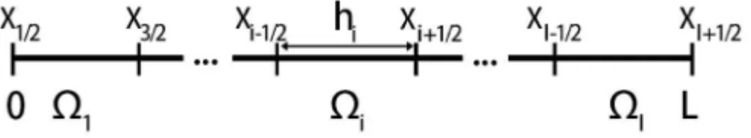
In general, to obtain the numerical solution for differential equations systems, the domain dis-cretization is required. At this point, we define a spatial mesh with total lengthLandIelements calledi,i=1: I, each one with lengthhi. The representation of this spatial mesh can be seen in Figure 1.
Figure 1: Spatial mesh in the domain of lengthL.
Now, we write the equations (2.1) and (2.2) in discretized form for each elementiin the domain
d J(x)
d x +aiφ (x)=
1
ke f f
νf iφ (x), (2.4)
J(x)= −Di
dφ (x)
then, the Albedo boundary conditions, equations (2.3), appear in the following discretized form
J1/2= −αLφ1/2, JI+1/2=αRφI+1/2.
The next step is to obtain the spatial balance equations for the zero and first order moments in each elementi. Thus, we need to apply the operator
2l+1
hi
xi+1/2
xi−1/2
•Pl
2(x−xi)
hi
d x,
in the equations (2.4) and (2.5). This operator is based in the Legendre polynomials [1], where
Pl represents the polynomial ofl degree. For the zero order balance equations,l =0, the Leg-endre polynomial is a constant, P0(x)=1. For first order,l =1, we have a linear polynomial,
P1(x)=x.
The balance equations, for the zero order moment appear in the following form
1
hi
(Ji+1/2−Ji−1/2)+aiφi = 1
ke f f
νf iφi,
Ji = −
Di
hi
(φi+1/2−φi−1/2),
where, the element average flux is
φi = 1
hi xi+1/2
xi−1/2
φ (x)d x, (2.6)
and the element average current is
Ji = 1
hi xi+1/2
xi−1/2
J(x)d x.
For the first order balance equations we have the following expressions
3
hi
(Ji+1/2+Ji−1/2−2Ji)+aiφi = 1
ke f f
νf iφi,
Ji = − 3Di
hi
(φi+1/2+φi−1/2−2φi),
where, the flux first order moment is
φi = 3
hi xi+1/2
xi−1/2
2(x−xi)
hi
φ (x)d x, (2.7)
and the the neutron current first order moment is defined as
Ji = 3
hi xi+1/2
xi−1/2
2(x−xi)
hi
3 THE FEM-SGF FORMULATION
The hybrid formulation proposed (FEM-SGF) in this paper combines two methods found in the literature. One of these methods is the FEM that obtains the solution of the diffusion model for eigenvalue problems using approximation functions. In this work, we choose two linear ap-proximation functions, one for the neutron flux and the other for neutron current, such functions satisfy the conditions described by integral equations in the domain. The other method that com-poses the hybrid formulation is the one-dimensional SGF [2], this method, reaches the solution of the diffusion equation with two spectral parametersαiandβi, obtained by spectral analysis of the mathematical model. Thus, the hybrid formulation proposed is based on the combination of linear approximation of the FEM with the approach quasi-analytic of the SGF.
The approximation functions of the FEM-SGF method appear in the following form
φ (x)=αiφi+ 2βi
hi
(x−xi)φi, (3.1)
J(x)=αiJi+ 2βi
hi
(x−xi)Ji, (3.2)
where, we introduce the spectral parameters of the SGF in the linear functions of the FEM.
To obtain the discretization of the approximation functions for the FEM-SGF, we need to evaluate those functions into the element edges. For the elements belonging to left half of the domain, we evaluate the functions (3.1) and (3.2) in the element right edge,xi+1/2, these functions discretized appear as
φi+1/2=αiφi+βiφi, (3.3)
Ji+1/2=αiJi+βiJi. (3.4)
For the elements in the right half of domain, the functions (3.1) and (3.2) are evaluated in the element left edge and the result is
φi−1/2=αiφi−βiφi, (3.5)
Ji−1/2=αiJi−βiJi. (3.6)
When the mesh has an odd number of elements, we must equate the average flux in equa-tions (3.3) and (3.5), and the average current in equaequa-tions (3.4) and (3.6), inside the central element to ensure the symmetry conditions in the domain. The resulting equations are
2βiφi−φi+1/2+φi−1/2=0,
2βiJi−Ji+1/2+Ji−1/2=0.
These solutions can be calculated by the spectral analysis, a technique proposed by Case and Zweifel [8]. The general analytical solutions can be write as
φ (x)=k1ex/µi +k2e−x/µi,J(x)=k1 −Di
µi
ex/µi +k
2
Di µi
e−x/µi,
wherek1 andk2 are arbitrary constants, and µi are the eigenvalues of the problem. The arbi-trary constants must be used to preserve the DE general analytical solution inside each spatial elementi.
Next, we can choose, arbitrarily, any of the functions in the general solution, because both func-tions carry the arbitrary constants k1 andk2, then, we select the functionφ (x), equation (3). The next step is to obtain the fluxes on the edgesφi±1/2, by evaluating (3) in the element edges (xi±1/2), which appears as
φi±1/2=k1exi/µie±hi/2µi +k2e−xi/µie∓hi/2µi, (3.7)
at this point, we calculate the average flux φi, by substituting (3) in the definition (2.6), the result appears as
φi =k1 µiexi/µi
hi
ehi/2µi −e−hi/2µi+k
2
µie−xi/µi
hi
ehi/2µi −e−hi/2µi, (3.8)
finally, we calculate the first order moment of neutron fluxφi, by substituting (3) in the defini-tion (2.7). The result appears in the following form
φi = k1
3µiexi/µi
hi
ehi/2µi+e−hi/2µi−k
1
6µ2iexi/µi
h2i
ehi/2µi −e−hi/2µi
−k2
3µie−xi/µi
hi
ehi/2µi+e−hi/2µi+k
2
6µ2ie−xi/µi
h2i
ehi/2µi −e−hi/2µi.
(3.9)
Now, we can substitute the expressions forφi±1/2,φi andφi, equations (3.7), (3.8) and (3.9), in (3.3) or (3.5) and write these in the form
k1(A−C)+k2(B−D)=0, (3.10)
where,
A=exi/µie±hi/2µi,
B=e−xi/µie∓hi/2µi,
C=αi µiexi/µi
hi
ehi/2µi −e−hi/2µi+β i
3µiexi/µi
hi
ehi/2µi +e−hi/2µi
−βi
6µ2iexi/µi
h2i
D=αi
µie−xi/µi
hi
ehi/2µi −e−hi/2µi−β i
3µie−xi/µi
hi
ehi/2µi +e−hi/2µi
+βi
6µ2ie−xi/µi
h2i
ehi/2µi −e−hi/2µi
.
But, the general analytical solutions must be preserved for anyk1andk2values, thus, (3.10) will be satisfied ifA=CandB= D. These equalities provide a linear system that lets us calculate the parametersαi andβi. The eigenvalueµi can be real or pure imaginary, thus, we can have two possible solutions,
(i) Ifai > 1
ke f f νf i
αi =γicoth(γi), βi =
sinh(γi) 3 cosh(γi)
γi
−3 sinh(γi) γi2
; (3.11)
(ii) Ifai < 1
ke f f νf i
αi =γicot(γi), βi = −
sin(γi) 3 cos(γi)
γi
−3 sin(γi) γi2
; (3.12)
whereγi = hi/2µi. The equations (3.11) and (3.12) used to calculate the parameters of aux-iliary equations, ensure, that the general analytical solutions are preserved inside each spatial elementi.
The algebraic linear equation system obtained by FEM-SGF is formed by (6I+2) unknowns and the same number of discretized equations. In this system we can eliminate the average element flux and the current (φi and Ji). Also, we can remove the first order moment of the flux and the current (φi andJi). Thus, we obtain an equivalent and reduced equation system of (2I +2) order. The reduced system, represents an eigenvalue problem, then, we can use direct or iterative techniques [7] to obtain the neutron flux distribution and the power method [7] to estimate the effective multiplication coefficient.
4 RESULTS AND DISCUSSION
In order to quantify the accuracy and the computational performance of the developed method, we compare the proposed formulation with conventional methods, specifically, the Diamond Difference method (DD) [17] and FEM method. DD is considered a fine mesh method and it has a low computational performance.
boundary conditions are reflexive in the left boundary and vacuum (αR = 0.5) in the right boundary. The convergence criterion requires that the relative deviation between two estimates of the effective multiplication factor to be less than or equal to 10−4%. The nominal power considered in the reactor is 10M W.
Table 1: Materials and geometric parameters of benchmark problem.
D(cm−1) a(cm−1) νf (cm−1) lengt h(cm)
Region 1 1 0,24 0,2733 25
Region 2 1,3 0,22 0,2565 25
Region 3 1 0,44 0,17 30
Region 4 1,3 0,1726 0,23 15
Region 5 2,7 0,046 0,015 30
Region 6 1 0,3 0,3526 25
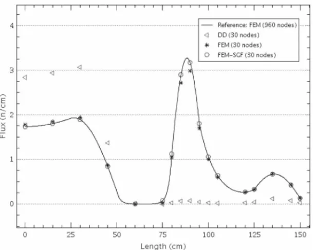
The numerical results for neutron flux distribution appear in Figures 2 and 3. The reference solution was generated using a fine mesh composed of 960 elements with the FEM method. The Figure 2 shows the behavior of the neutron flux in the domain and the Figure 3 presents the relative deviations of the three methods with respect to reference solution. As we see, in this benchmark problem appear strong neutron flux gradients in some regions. Consequently, most of the numerical methods fail to obtain accurate results.
Figure 2 shows that the FEM-SGF method, with a coarse mesh (30 elements), keeps the neutron flux close to reference solution, while the FEM, with the same mesh, moves away from the reference solutions in the regions with strong gradients. On the other hand, the DD method generates meaningless results for a coarse mesh calculations.
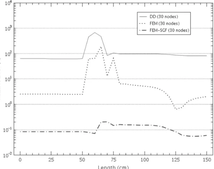
The differences between numerical results obtained by the three methods can be more noticeable in Figure 3. The strongest variation of the neutron flux occurs in the region between x = 50 and x = 75. In this region the numerical methods find the major difficulty to estimate the neutron flux. The FEM-SGF presents the smallest relative deviations, 0.01% approximately, while in the FEM the relative errors vary between 1% to 100%. The relative errors associated to DD are even higher.
Figure 3: Relative deviations in neutron flux distribution for DD, FEM and FEM-SGF methods in coarse mesh.
To analyze the reactor power density results, we choose the region between x = 60 and
x = 100cm, which presents a strong gradient in the neutron flux and a high neutron density. The Table 2 shows the results for the power density and the relative deviations for each method.
Table 2: Numerical results for power density in the region (60≤x≤100)for DD, FEM and FEM-SGF methods in coarse mesh.
Method (elements) Power (MW) Rel. deviation (%)
DD (30) 6.208733E-02 9.769013E+01
FEM (30) 2.523533E+00 6.115466E+00
FEM-SGF (30) 2.692115E+00 1.563635E-01
Reference: FEM (960) 2.687912E+00 ...
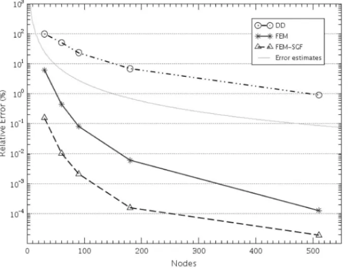
In the Figure 4, we present the relative deviation behavior, in power density calculations, as a function of the element number for all the discussed formulations. In general, we can see that the FEM-SGF reached the best results if compared with the conventional methods, for all spatial meshes considered. Specifically, when we compare the FEM-SGF with the FEM, we notice that it shows similar results with about 1/3 of the elements of the FEM. Therefore, the FEM-SGF is as accurate, using a coarse mesh, as the DD in fine mesh and the FEM in intermediate mesh. To complete this analysis, we compare the behavior of the relative deviation with the error ana-lytical estimates for the analyzed methods (Fig. 4). The convergence order of the DD, FEM and FEM-SGF methods, in asymptotic notation is O(h2)[6, 17]. We can also see in Figure 4, that the curves of each method have similar behaviors modified by some multiplicative constant.
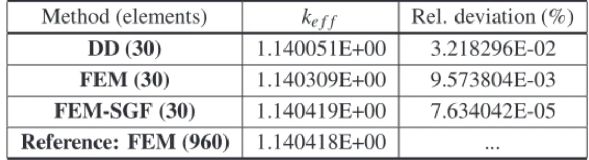
The numerical results for the effective multiplication coefficient (ke f f) appear in Table 3. The
ke f f value obtained by FEM-SGF have the smallest relative deviation, 10−5%, approximately. The results for the conventional methods (FEM and DD), suffer a bigger influence of the spatial grid dimensions. They present relative errors of 10−3% and 10−2%, respectively.
Table 3: Numerical results for effective multiplication coefficient for DD, FEM and FEM-SGF methods in coarse mesh.
Method (elements) ke f f Rel. deviation (%)
DD (30) 1.140051E+00 3.218296E-02
FEM (30) 1.140309E+00 9.573804E-03
FEM-SGF (30) 1.140419E+00 7.634042E-05
Reference: FEM (960) 1.140418E+00 ...
To characterize the FEM-SGF computational performance, we consider the dominant operation in the algorithmic implementation of the numerical formulations. This dominant operation is associated with the solution of the algebraic linear system generated by the discretization pro-cedure in each method. The resulting matrices in the spatial discretization process are sparse, specifically, they are banded symmetric [7]. The bandwidth for DD, FEM and FEM-SGF meth-ods are 3, 4 and 4, respectively. Thus, considering the dominant operation, the computational cost associated to the numerical formulations DD, FEM and FEM-SGF, in asymptotic notation, is O(M)O(I), whereM is the iteration number of power method for eigenvalue convergence. It is noteworthy that the DD generate an algebraic linear system with (I+1) variables and equa-tions, and the order of algebraic linear system generated by FEM is equivalent to FEM-SGF. Moreover, due to the specific characteristic of the FEM-SGF, the matrix coefficients depend on problem eigenvalue and must be updated on each iteration.
5 CONCLUSIONS AND FUTURE WORKS
We presented in this work a hybrid formulation to solve the one-dimensional neutron diffusion equation in multiplying media and one energy group. The hybrid character of this formulation is based on the combination of the FEM linear approximations with the SGF spectral parameters. These parameters allow us to preserve the general analytic solutions inside each element. The FEM-SGF formulation, permits to obtain accurate numerical results in coarse mesh, suggesting a high computational performance.
formulation using a coarse mesh presents the same precision than the compared methods with finer meshes and, for that reason, it has the better computational performance.
As future works, we suggest to reduce the FEM-SGF algebraic linear system order to (I+1). We also suggest to extend the hybrid formulation to solve multi-dimensional problems, and consider multi-group approximations.
ACKNOWLEDGMENTS
Authors acknowledge to Conselho Nacional de Desenvolvimento Cient´ıfico e Tecnol´ogico (CNPq, BRAZIL) and Fundac¸˜ao de Amparo `a Pesquisa do Estado da Bahia (FAPESB, BRAZIL) for the financial support provided. Also, the authors acknowledge the Universidade Estadual de Santa Cruz, for supporting this research and the N´ucleo de Biologia Computacional e Gest˜ao de Informac¸˜oes Biotecnol´ogicas for offering the infrastructure for the development of the computational experiments.
RESUMO. A utilizac¸˜ao de centrais nucleares para gerac¸˜ao de energia el´etrica ´e uma das
principais alternativas para atender a demanda energ´etica nos pr´oximos anos sem agravar os problemas ambientais associados ao aquecimento global. O uso de m´etodos e t´ecnicas de
simulac¸˜ao que estimem a populac¸˜ao de nˆeutrons no n´ucleo ´e fundamental para garantir a operac¸˜ao segura e confi´avel do reator. Neste trabalho apresentamos uma formulac¸˜ao h´ıbrida
para resolver problemas de autovalor de difus˜ao de nˆeutrons em dom´ınios unidimensionais
e aproximac¸˜ao de uma velocidade. Esta formulac¸˜ao combina a simplicidade do M´etodo de Elementos Finitos com uma aproximac¸˜ao Espectro-Nodal e permite obter resultados
pre-cisos em c´alculos de malha grossa. A precis˜ao e o desempenho computacional do m´etodo
proposto s˜ao caracterizados atrav´es da soluc¸˜ao de um problema modelo com alto grau de heterogeneidade.
Palavras-chave:Problemas de autovalor, Equac¸˜ao de difus˜ao de nˆeutrons, Func¸˜ao espectral
de Green.
REFERENCES
[1] R.E. Attar. “Legendre Polynomials and Functions”. CreateSpace, (2009).
[2] R.C. Barros & E.W. Larsen. A Numerical Method for Multigroup Slab-Geometry Discrete Ordinates Problems with No Spatial Truncation Error.Transport Theory and Statistical Physics,20(1991), 441–462.
[3] R.C. Barros & E.W. Larsen. A spectral nodal method for one-group X,Y-geometry discrete ordinates problems.Nuclear Science and Engineering,111(1) (1992), 34–45.
[5] G.I. Bell & S. Glasstone. “Nuclear reactor theory”. Van Nostrand Reinhold Co., (1970).
[6] S.C. Brenner & L.R. Scott. “The Mathematical Theory of Finite Element Methods”. Springer-Verlag New York, Inc., (1996).
[7] R.L. Burden & D.J. Faires. “Numerical Analysis”. Ninth Edition, BROOKS/COLE – CENGAGE Learning, (2011).
[8] K.M. Case & P.F. Zweifel. “Linear transport theory”. Addison-Wesley Pub. Co., (1967).
[9] C. Ceolin, M. Schramm, B.E.J. Bodmann, M.T. Vilhena & S.B. Leite. On an analytical evaluation of the flux and dominant eigenvalue problem for the steady state multi-group multi-layer neutron diffusion equation.Kerntechnik,79(2014), 430–435.
[10] D.S. Dominguez & R.C. Barros. The spectral Green’s function linear-nodal method for one-speed X,Y-geometry discrete ordinates deep penetration problems.Annals of Nuclear Energy,34(2007), 958.
[11] D.S. Dominguez, C.R.G. Hernandez & R.C. Barros. Spectral nodal method for numerically solving two-energy group X,Y geometry neutron diffusion eigenvalue problems.International Journal of Nuclear Energy, Science and Technology (Print),5(2010), 66.
[12] J.J. Duderstadt & L.J. Hamilton. “Nuclear Reactor Analysis”. John Wiley & Sons Inc, (1975).
[13] Empresa de Pesquisa Energ´etica. “Plano Nacional de Energia 2030”, Minist´erio de Minas e Energia, Rio de Janeiro, Brasil, (2007).
[14] T. Hayashi & D. Inoue. Calculation of leaky Lamb waves with a semi-analytical finite element method.Ultrasonics,54(6) (2014), 1460–1469.
[15] J.D. Jung & W. Becker. Semi-analytical modeling of composite beams using the scaled boundary finite element method.Composite Structures,137(2016), 121–129.
[16] J.R. Lamarsh & A.J. Baratta. “Introduction to Nuclear Engineering”. Prentice Hall, (2001).
[17] E.E. Lewis & W.F. Miller Jr. “Computational Methods of Neutron Transport”. American Nuclear Society, Illinois, USA, (1993).
[18] P. Liu, D. Wang & M. Oeser. Application of semi-analytical finite element method coupled with infinite element for analysis of asphalt pavement structural response.Journal of Traffic and Trans-portation Engineering (English Edition),2(1) (2015), 48–58.
[19] E. Sauter, F.S. Azevedo, M. Thompson & M.T. Vilhena. Eigenvalues of the Anisotropic Transport Equation in a Slab.Transport Theory and Statistical Physics, (2012), 448–472.
[20] E. Sauter, F.S. Azevedo, M. Thompson & M.T.M.B. Vilhena. Solution of the one-dimensional trans-port equation by the vector Green function method: Error bounds and simulation.Applied Mathemat-ics and Computation,219, (2013), 11291–11301.
[21] A.C. da Silva, A.S. Martinez & A. da C. Gonc¸alves. Reconstruction of the Flux in a Slab Reactor. World Journal of Nuclear Science and Technology, (2012), 181–186.
[22] W.M. Stacey. “Nuclear Reactor Physics”, Wiley-VCH, (2007).