Jump Dominance on the Contaminant Transport
Residual Error Estimator*
J.P. MARTINS1**, A. FIRMIANO2 and E. WENDLAND1
Received on November 10, 2013 / Accepted on April 9, 2014
ABSTRACT.Considering the fact that the transport of contaminants occur in small advection regime, a residual estimator is used to evaluate the parabolic equation that describes the phenomena of advection-diffusion-reaction in the saturated porous medium. The correspondent numerical solution is obtained by the finite element method using theθ A-stable scheme and a Python code. The residual error estimator considers its component parts and enables analysis and comparisons of contributions to residual error. This analysis considers a problem sequence with a different number of elements in computational mesh. As a result of numerical simulations, there is a dominance of the jump residuals compared to other resid-ual estimates and this dominance increases with both, the growth of elements number in the computa-tional mesh and with time. Furthermore, the considered problem requires addicomputa-tional effort for the calcu-lation of contributions associated with theL2projection of the contaminant source function on the finite element space.
Keywords:residual error estimator, advection-diffusion-reaction equation, small advection regime, finite elements, contaminant transport in porous media.
1 INTRODUCTION
Analytical solutions are far from encompassing the variety of phenomena present in contam-inant transport and numerical methods are required to obtain an approximate solution of the corresponding mathematical model. Moreover, the reliability of computational methods depends on the discretization technique and the quality of the finite element mesh adopted. Although es-timates ofa prioriare available,a posterioriestimates are fundamental for practical problems involving finite element method [13]. Once the numerical result is obtained, thea posteriori
error estimator can be used to provide general or specific information about the quality of the numerical solution [3].
*Paper presented at CMAC-SE 2013.
**Corresponding author: Jo˜ao Paulo Martins dos Santos
1Department of Hydraulics and Sanitary Engineering, EESC – USP, Av. Trabalhador Sancarlense, 400, 13566-590 S˜ao Carlos, SP, Brazil. E-mails: [email protected]; [email protected]
2 THE MODEL PROBLEM FOR THE CONTAMINANT TRANSPORT
The linear second order parabolic equation is used to describe the contaminant transport in a domain⊂R2, with general unknown concentration solutionC =C(x,y,t), data functions D,v, λ, f,g,C0and final timetf inal is arbitrary, but is kept constant.
The data are real valued functions that may depend on space and time while the initial con-dition depends only on space [17]. Here, the equation describes the phenomena of advection-dispersion-reaction (ADR model) in a saturated porous media and, according to [1], can be pre-sented by:
∂tC−div(D∇C)+v· ∇C+λC= f in ×(0,tf inal]
C=0 in ŴD×(0,tf inal]
n·D∇C=g in ŴN×(0,tf inal]
C=C0 in for t=0 (2.1)
where ⊂ R2 is a polygonal cross-section with a Lipschitz boundary Ŵ consisting of two disjoint partsŴD andŴN. The space dependent functionC = C0infort =0 is the initial condition while
C=CD in ŴD×(0,tf inal] and n·D∇C =g in ŴN×(0,tf inal]
are the Dirichlet and Neumann boundary conditions. Assuming that the data satisfy the addi-tional conditions [20]:
P1 – The dispersionD=D(x,y,t)is a continuously differentiable matrix-valued function and symmetric, uniformly positive definite and uniformly isotropic. Formally,
ε= inf 0≤t≤tf inal,(x,y)∈
min
R2−{0}
zTD(x,y,t)z
zTz >0, (2.2)
and
κ =ε−1 sup 0≤t≤tf inal,(x,y)∈
max
z∈R2−{0}
zTD(x,y,t)z
zTz (2.3)
is moderate size constant.
P2 – The velocityv = v(x,y,t) = (vx(x,y,t), vy(x,y,t))is a continuously differentiable
vector-field and scaled such that
sup 0≤t≤tf inal,(x,y)∈
|v(x,y,t)| ≤1.
P4 – There is a constantβ such thatλ−(1/2)div(v)≥β for almost all(x,y)∈ and 0 ≤ t ≤tf inal. Moreover there is and a constantcb≥0 of moderate size such that
sup 0≤t≤tf inal,(x,y)∈
|λ(x,y,t)| ≤cbβ.
P5 – The Dirichlet boundaryŴD has positive measure (d −1)-dimensional and includes the
inflow boundary
0<t≤tf inal
{(x,y)∈Ŵ:v·n(x,y) <0}.
With these additional assumptions, the contaminant transport regime can be classified into:
• dominant dispersion:
sup 0≤t≤tf inal,(x,y)∈
|v(x,y,t)| ≤ccε and β≤c,ε; (2.4)
with constants of moderate size;
• regime of dominant reaction:
sup 0≤t≤tf inal,(x,y)∈
|v(x,y,t)| ≤ccε and β≫ε; (2.5)
with a constantccof moderate size;
• regime of dominant advection:cv≫ε.
A detailed discussion of these elements can be found in D. Praetorius [17] which is an extension of the results from Verf¨urth [20].
To derive the space-time discretization of (2.1), we consider a test functionw ∈ HD1()where
HD1()denotes the subspace of the Sobolev spaceH1()=W1,2(), with functions that vanish on the Dirichlet boundaryŴD. Multiply equation (2.1) by a test function and use integration by
parts to derive the weak form
(∂tCw+ ∇C·D∇w+v· ∇Cw+λCw)d=
fwd+
ŴN
gwd S. (2.6)
Next, consider the partitionI = {[tn−1,tn] :1n NI}of the time interval[0,tf inal]such
that 0=t0<t1. . . <tNI =tf inal.
For everynwith 1n NI denote byIn = [tn−1,tn]then-th subinterval andτn =tn−tn−1 its length.
With every intermediate timetn, 0n NI associate an admissible, affine equivalent, shape
• ∪Ŵis the union of all elements inTn;
• Affine equivalence, Admissibility and Shape-regularity;
• Non-degeneracy, transition condition and degree condition.
With a time discretization parameterθ ∈ [12,1]and the abbreviationsCn =C(x,y,tn),Dn =
D(x,y,tn),vn = v(x,y,tn), λn = λ(x,y,tn), fn = f(x,y,tn), gn = g(x,y,tn)the finite
element approximation withθ-A-stable-scheme is obtained by replacing the approximations in the weak form of the parabolic problem and is given by
FindCn∈ Xn,0≤n ≤NI, such thatC0=π0C0and forn=1,2, ...,NI
1
τn
(Cn−Cn−1)wnd+
(θ∇Cn+(1−θ )∇Cn−1)·Dn∇wnd
+
vn· ∇(θCn+(1−θ )Cn−1)wnd+
λn(θCn+(1−θ )Cn−1)wnd
=
fn+(1−θ )fn−1wnd+
ŴN
(θgn+(1−θ )gn−1)wnd Sfor allwn∈Xn.
(2.7)
whereCn =CTn
n andwn=wTn.
In particular,θ =1/2 gives theCrank-Nicolson schemeandθ =1 givesimplicit Euler scheme
[20]. Thus, finite element formulation (2.7) can be rewritten asa(Cnn, wn)= L(wn). The term a(Cnn, wn)is called the bilinear form and is defined by expression (2.8)
a(Cn, wn) =
1
τn
Cnwnd+
(θ∇Cn)·Dn∇wnd
+
vn· ∇(θCn)wnd+
λn(θCn)wnd
+
ŴN
θgnwnd S,
(2.8)
while the termL(wn)is called linear form and defined by expression (2.9)
L(wn) =
1
τn
Cn−1wnd+
((θ−1)∇Cn−1)·Dn∇wnd
+
vn· ∇((θ −1)Cn−1)wnd+
λn((θ−1)Cn−1)wnd
+
(θfn+(1−θ )fn−1)wnd+
ŴN
(1−θ )gn−1wnd S
(2.9)
A detailed description of the residual estimator and assumptions presented here are in references [20, 19, 16, 17]. For finite elements method, a detailed discussion can be found in reference [2].
In the residual method, an element residualsRK is defined by:
RK = fI −
1
τn
Cn−Cn−1+div(Dn∇(θCn+(1−θ )Cn−1)) −vn· ∇(θCn+(1−θ )Cn−1)−λn(θCn+(1−θ )Cn−1)
(2.10)
while an edge or face residualRE is defined by:
RE =
⎧ ⎪ ⎨ ⎪ ⎩
−JE(nE·Dn∇(θCn+(1−θ )Cn−1)) if EŴ gI−nE·Dn∇(θCn+(1−θ )Cn−1) if E⊂ŴN
0 if E⊂ŴD
(2.11)
whereJis the jump operator, fI(x,y,t)=πn(θf(x,y,tn)+(1−θ )f(x,y,tn−1))andgI(x, y,t) = πn(θg(x,y,tn)+(1−θ )g(x,y,tn−1))the projection functions on the finite element spaceXn[20]. According to Verf¨urth [20], if the transport regime is of small advection then the
residual estimator is given by equation (2.12)
ˆ ηI =
C0−π0C0
2
L()+ NI
n=1 τnηn
2
+Cn−Cn−12 1 2 (2.12) where
ηnT
n
2
=
K
α2KRK
2
L2(K)+
E
ε−12αERE
2
L2(E), (2.13)
and
Cn−Cn−12=ε∇(Cn−Cn−1)
L2()+β
Cn−Cn−1
L2(), (2.14)
with weighting factorsαS = min{hSε−
1 2,−β
1
2}, whereS = {K,E}is an element or an edge/ face andβ−12 = ∞ifβ=0.
3 IMPLEMENTATION
The Python numerical code considers the available methodology for the FEniCS Project. A complete description of this project can be found in references [8, 9, 10, 11, 12, 14] or at http://fenicsproject.org [4]. For graphical display of numerical solutions, Matplotlib/Scitools was used [15, 18]. Using Python language, the contaminant transport equation is implemented using the available tools from [4]. These tools provide conditions for setting the transport of contami-nants directly through the use of bilinear and linear forms. Furthermore, mesh, initial conditions, dispersions, velocity field, projections and boundary conditions are defined using the available classes/tools described in documentation [4]. For example,mesh =U nit SquareMesh(nx,ny,
‘crossed′)gives a mesh withnx,nytriangular elements in each coordinate direction andcrossed
After the solution in then-th step is obtained, the residual error estimates (2.13) are implemented through the summation of the quantities defined in (2.10) and (2.11). Formally,
ηnT
n
2
=
K
α2KRK
2
L2(K)
E Cn
+
EŴ
ε−12αERE2
L2(E)
J Cn
+
E⊆ŴN
ε−12αERE2
L2(E)
BCn
. (3.1)
According to the designations adopted by Verf¨urth [20] and D. Praetorius [17], components
ECn, J Cn, BCn,Cn −Cn−12will be called, respectively: element, jump, boundary and time contributions for then-th time step. These quantities allow us to rewrite equation (2.12) as a sum of spatial and temporal contributions, obtained in each step, weighted by time step. Formally,
ˆ ηI =
C0−π0C0
2L
()+ NI
n=1
τn(E Sn)2
12
. (3.2)
From equation (3.2), the amount(E Sn)2 =(ηn)2+Cn −Cn−12may be regarded as the residual error at each time step.
The code that implements the element, jump, boundary and time contributions follows an exam-ple available in [6]. This allows the calculation ofηI and enables comparisons of components or
individual evaluation of contributions. This paper considers:
• Jump contribution versus element contributionRnJ um p/Element, defined by
RnJ um p/Element = J C
n
ECn =
EŴ
ε−12αERE
2
L2(E)
K
α2KRK
2
L2(K)
(3.3)
which provides information on the magnitude of the jumps on the elements;
• Time contributions weighted by time time step, defined by τn
Cn −Cn−12 which
provides information on time residual error.
4 RESULTS AND DISCUSSION
With an adaptation of a problem described in [7] and [17], this paper implements the contam-inant transport equation in a two-dimensional rectangular domain defined by points x = (x,y) ∈ R2
. A spatial adaptation of that problem consider defined by points(x0,y0) = (0,0),(x1,y0) = (80,0), (x1,y1) = (80,40)and(x0,y1) = (0,40), inital conditionC0 = C(x,y,0)=0 and contaminant source f defined by
f(x,y,t)=
1 if 9.375x 1.625, 19.375y20.625
The physical parameters are the velocity fieldv = (vx, vy) = (0.864,0)md, the dispersion D = αDvxI2×2with I2×2 the identity matrix of order two and αD = 0.05m the diffusivity.
Neumann boundary condition is defined, using bilinear and linear forms, byg =n·D∇C on
ŴN = {x1} ×(y0,y1)while Dirichlet boundaries are defined, using the available class, byC =0 onŴD =ŴŴN.
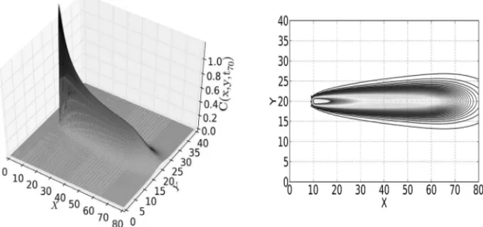
For alltn,1 n NI, the numerical result of contaminant transport provides the distribution
functionCn ∈R2, which describes the contaminant concentration at each point of. Figure (1) presents the numerical solution fort70 = 70days,τn = 1.0day, lagrangian functions of order
two,θ=1.0 and finite element mesh withnx=200=2nytriangular elements in each direction
andleft/rigthorientation.
Figure 1: Numerical solution and level curves fort70 =70dayswithτn =1.0day, lagrangian
functions of order two, θ = 1.0 and finite element mesh withnx = 200 = 2ny triangular
elements in each direction andleft/rigthorientation.
For residual estimates, the conditionsP1-P5were verified and contaminant transport was classi-fied in advection dominated [17]. However, the regime is the small advection sinceCc =v/ǫis
a constant of moderate size [5].
The numerical simulations consider finite element meshes withnx =2nytriangular elements in
each coordinate direction withleft/rightorientation,τn=0.50,tf inal =100.0days,θ =1.0 and
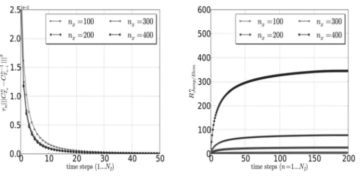
lagrangian functions of order two. Figures (2)-a and (2)-b presents the results for temporal esti-mates and for ratioRnJ um p/Element for a sequence of problems withnx = [100,200,300,400].
Numerical results provide that temporal residual decreases with time and as the number of el-ements in mesh increases. On the other hand, RnJ um p/Element increases with time and as the number of elements in mesh increases. The increasing inRnJ um p/Element with time is due to the contaminant front advances, which, in turn, reflects in the dominance of jump contributions un-der element contributions already in the coarse mesh. This dominance characterizes the jump contributions as the most relevant part ofηI becauseτn
Figure 2: Temporal contributionsτn
Cn−Cn−12and the ratioRnJ um p/Element =J Cn/ECn
forτn = 0.50,tf inal = 100days,θ = 1.0, lagrangian functions of order two,nx =2ny =
[100,200,300,400].
With the results,ηI can be approximated by
ˆ ηI =
C0−π0C0
2
L+ NI
n=1
τn(E Sn)2
12 =
NI
n=1
τn(J Cn)2
12
(4.2)
whereC0−π0C0
2
L() =0 and(E S
n)2=(ηn)2+Cn−Cn−12≈ECn+J Cn≈J Cn.
This results and the approximation forηI reveals that jump error is not a negligible quantity and
complements the results obtained by Firmiano [5]. In fact the jump residual can be the most important part of the residual estimates.
5 CONCLUSION
The presence of residual estimates enables an analysis of the numerical solution, which provides information about the quality of the numerical results. Error estimator partition allows us to analyze and compare the component parts of residual error. This provides a better understand-ing of residual behavior for changunderstand-ing number of elements in mesh or time step. As a result of simulations, jump dominance manifests for all adopted meshes, which is due to the advances of contaminant front in the computational domain. As the number of finite elements increases, the magnitude of dominance becomes more significant, making elements and temporal contribu-tions negligible when compared to jump residual. This dominance shows that jump residual is a important quantity in residual error estimator and can not be neglected.
que descreve o fenˆomeno de advecc¸˜ao-difus˜ao-reac¸˜ao em meio poroso saturado. A soluc¸˜ao
num´erica correspondente ´e obtida pelo m´etodo de elementos finitos usando um esquema
θA-est´avel em c ´odigo Python. O estimador de erro residual avalia separadamente as partes
componentes do erro e permite a an´alise e comparac¸˜ao das contribuic¸ ˜oes para o erro residual.
Essa an´alise considera uma sequˆencia de problemas com diferentes n´umeros de elementos na malha computacional. As simulac¸ ˜oes num´ericas indicam que o residual do salto ´e dominante
em comparac¸˜ao com outros res´ıduos estimados e a dominˆancia cresce com o n´umero de
ele-mentos na malha e com o tempo. Adicionalmente, o problema considerado requer esforc¸o adicional para o c´alculo das contribuic¸ ˜oes associadas com a projec¸˜aoL2da func¸˜ao fonte de
contaminante no espac¸o de elementos finitos.
Palavras-chave:estimador de erro residual, equac¸˜ao de advecc¸˜ao-difus˜ao-reac¸˜ao, regime de pequena advecc¸˜ao, elementos finitos, transporte de contaminantes em meios porosos.
REFERENCES
[1] J. Bear. Hydraulics of Groudwater, Dover Publications Inc., New York, (1979).
[2] S.C. Brenner. The Mathematical Theory of Finite Element Methods, em “Texts in Applied Mathe-matics, v.15” (J.E. Marsden, L. Sirovich and S.S. Antman, eds.), Springer-Verlag, New York, (1994).
[3] R.E. Ewing.A posteriorierror estimation.Computer Methods in Applied Mechanics and Engineering,
82(1-3): 59–72, September (1990).
[4] Fenics project documentation.http://fenicsproject.org/, 2012. Accessed in 05/2012.
[5] A. Firmiano. “Um estimador de erroa posterioripara a equac¸˜ao do transporte de contaminantes em regime de pequena advecc¸˜ao”. Tese de Doutorado, SHS/EESC/USP, (2010).
[6] https://answers.launchpad.net/dolfin/+question/177108.
[7] G. Hofinger & F. Judex. Pollution in groundwater flow: definition of ARGESIM comparison C19. Simulation News Europe, 44/45: 51–52, (2005).
[8] R.C. Kirby. Algorithm 839: Fiat, a new paradigm for computing finite element basis functions.ACM Transactions on Mathematical Software,30(4) (2004), 502–516.
[9] R.C. Kirby. Optimizing the evaluation of finite element matrices.SIAM Journal on Scientific Com-puting,27(3) (2005), 741–758.
[10] R.C. Kirby. A compiler for variational forms.ACM Transactions on Mathematical Software,32(3), (2006).
[11] R.C. Kirby. Efficient compilation of a class of variational forms.ACM Transactions on Mathematical Software,33(3), (2007).
[12] R.C. Kirby. Geometric optimization of the evaluation of finite element matrices.SIAM Journal on Scientific Computing,29(2) (2007), 827–841.
[14] A. Logg. Automating the finite element method.Archives of Computational Methods in Engineer-ing,14(2) (2007), 93–138.
[15] Matplotlib. http://matplotlib.sourceforge.net/index.html, 2012. Accessed in 06/2012.
[16] A. Papastavrou.A posteriorierror estimators for stationary convection-diffusion problems: a compu-tational comparison.Computer Methods in Applied Mechanics and Engineering,189(2): 449–462, September (2000).
[17] D. Praetorius. A space-time adaptive algorithm for linear parabolic problems, Asc report 07/2008, Institute for Analysis and Scientific Computing Vienna University of Technology-TU Wien, 2008, dispon´ıvel em www.asc.tuwien.ac.at ISBN 978-3-902627-00-1.
[18] Scitools: Python library for scientific computing.http://code.google.com/p/scitools/, 2012. Accessed in 06/2012.
[19] R. Verf¨urth. A review ofa posteriorierror estimation techniques for elasticity problems.Computer Methods in Applied Mechanics and Engineering,176(1-4): 419–440, July (1999).
[20] R. Verf¨urth. Adaptive finite element methods lecture notes winter term 2007/08, 2007/2008,
dispo-n´ıvel em http://citeseerx.ist.psu.edu/viewdoc/summary-doi=10.1.1.155.