Particle image velocimetry and computational fluid dynamics applied to study the effect of hydrodynamics forces on animal cells cultivated in Taylor vortex bioreactor

(1)

Particle image velocimetry and computational ﬂuid

dynamics applied to study the eﬀect of hydrodynamics

forces on animal cells cultivated in Taylor vortex

bioreactor

Universidade Federal do São Carlor – UFSCar

Programa de Pós-Graduação em Engenharia Química – PPGEQ Laboratório de Technologia de Cultivo Celular – LATECC

Orientador: Prof. Dr. Claudio Alberto Torres Suazo

(2)

(3)

LABORATÓRIO DE TECHNOLOGIA DE CULTIVO

CELULAR

DEPARTAMENTO DE ENGENHARIA QUÍMICA

HARMINDER SINGH

PARTICLE IMAGE VELOCIMETRY AND

COMPUTATIONAL FLUID DYNAMICS APPLIED TO

STUDY THE EFFECT OF HYDRODYNAMICS FORCES

ON ANIMAL CELLS CULTIVATED IN TAYLOR

VORTEX BIOREACTOR

Tese

apresentado ao Programa de Pós-Graduação em Engenharia Química para obtenção do titulo de doutor em Engenharia Química.

Orientação: Prof. Dr. Claudio Alberto Torres Suazo

(4)

Ficha catalográfica elaborada pelo DePT da Biblioteca Comunitária UFSCar Processamento Técnico

com os dados fornecidos pelo(a) autor(a)

S617p

Singh, Harminder

Particle image velocimetry and computational fluid dynamics applied to study the effect of hydrodynamics forces on animal cells cultivated in Taylor vortex bioreactor / Harminder Singh. -- São Carlos : UFSCar, 2016.

203 p.

Tese (Doutorado) -- Universidade Federal de São Carlos, 2016.

(5)

(6)

Agradecimentos

First and foremost, I would like to sincerely thank the Almighty, the One True Lord, for blessing the knowledge, will power, patience and numerous other skills required to become a researcher. There are three direct contributors who have enabled me to reach this stage of completing this thesis: my supervisor Prof. Dr. Claudio A. T. Suazo, "doutorado sanduìche"supervisor Prof. Dr. Alain Liné and financial supporter CNPq, Brasil. Without the conjunction of these three stepping stones, this study would not have been feasible. For the financial support, i would like to offer my gratitude to the Conselho Nacional de Desenvolvimento Cientifico e Tecnologico (CNPq), Brasil for the postgraduate (processo nº 140756/2012-4) and "Doutorado Sanduíche"(processo nº - 241739/2012-8) Scholarship programs.

I am really grateful to Prof. Dr. Claudio A. T. Suazo for always having faith in my capabilities, giving me space and independence, and at the same time guiding me through whenever needed. His vast knowledge and experience in the ﬁeld of bioreactors always opened various doors when things looked bleak. Apart from his able guidance, friendliness and carefulness, his support will always be appreciated.

On the third front, i am indebted to Prof Dr. Alain Liné for accepting me as his "doutorado sanduìche"student, his support, care and participation in this work even now, long after the program ended in April 2014. Sharing of his wonderful ideas, vast knowledge and experience in the ﬁeld of hydrodynamics kept me alive and ticking, and gave direction every time i got a bit lost. Major part of this thesis work has been conducted under his able guidance, and his critique only enhanced the quality of this work.

I am thankful to Prof Dr. Roberto de Campos Giordano and Prof. Dr. José Antônio Silveira Gonçalves for their support, and sharing of their thoughts which helped in the improvement of this work. I am also grateful to all of the technicians, post-grads, and staﬀ of the Chemical Engineering department in making this an enjoyable place to work.

(7)

(8)

(9)

(10)

Resumo

O biorreator de Vórtices de Taylor (TVB) está se tornando uma nova descoberta, devido ao seu cisalhamento mais suave e fluxo homogêoneo em comparações com os biorretores de tanque agitados. Na literatura acadêmica há pouca informação sobre este biorreator quanto a taxa de dissipação de energia viscosa (VEDR), que é o parêmetro ideal para caracterizar a morte celular, e seus aspectos geométricos, que afetam o cultivo das células animais, resultando em baixa eficiência. A presente pesquisa, portanto, objetivou focar na estimativa da VEDR de fluxo médio e de energia cinética turbulenta (TKE) no TVB usando os métodos: experimental de 2D de velocimetria das partículas por imagem (PIV) e númerico de dinâmica de fluídos computacional (CFD) com diferentes modelos de turbulência, principalmente a simulação numérica direta (DNS). E focar nos aspectos geométricos do impacto da área de apuramento entre o cilindo interno e externo e na forma da base do cilindro externo na estrutura de fluxo do TVB.

Os dois métodos experimental e númerico demonstraram que, em aproximadamente 80 % da área lateral entre os cilindros interno e externo onde as células vão passar a maior parte do tempo, a magnitude de velocidade é de cerca de 50 % da máxima e os valores de VEDR são 10 vezes menores do que nas paredes. Qualitativamente, o DNS mostrou boas comparações dos fluxos médios e dos parâmetros turbulentos em relação aos resultados apresentados pelo PIV para o TVB. No entanto, quantitativamente, apenas as previsões médias de velocidade estão em boa concordância com os dados do PIV, pois os parâmetros turbulentos foram sub-estimados. Entre os diferentes modelos de turbulência utilizados, o modelo simulação de grande escala (LES) - Wall Adapting Local Eddy-Viscosity apresentou a melhor comparação com os dados do DNS para todos os parâmetros do fluxo. O modelo de estresse Reynolds e LES - Smagorinsky, por sua vez, apresentaram as piores comparações. Os modelos de duas equações de RANS, entretanto, apesar de estimarem bem os componentes de velocidade média em comparação com os dados do modelo DNS, não captaram bem as estruturas de fluxo dos componentes de turbulência. Quanto aos aspectos geométricos, as alterações nas características da área de apuramento entre o cilindo interno e externo e a estrutura curva da base do cilindro externo, que são de importância prática em tanque agitados, neste estudo, afetaram negativamente o fluxo no TVB devido ao seu baixo componente de velocidade axial. Por fim, a comparação entre o TVB e o Spinner Flask, considerado também um biorretor com baixo cissalhamento, demostrou que para Re/ReT semelhante, os valores máximo e médio do VEDR foram sempre inferiores, e devido à diferença muito menor entre o os valores máximo e médio, o TVB apresenta estruturas mais uniformes em comparação com o Spinner Flask.

(11)

(12)

Abstract

Taylor-Vortex reactor (TVB) is fast becoming the next bioreactor to culture animal cells due to milder shear and homogeneous flow structures through-out the bioreactor in comparison to the traditional stirred vessels. However, there is little information in the literature for the TVB on the viscous energy dissipation rate (VEDR), which is considered the ideal parameter to characterize the cell death, and its geometrical aspects, which may affect the culture of animal cells resulting in poor efficiency. Consequently, this work focuses on: the estimation of the VEDR of mean flow and turbulent kinetic energy (TKE) using an experimental 2D particle image velocimetry (PIV) method and a computational fluid dynamics (CFD) method using different turbulence models, principally the direct numerical simulation (DNS) model; and, the impact of the off-bottom clearance area and the external cylinder’s bottom shape on the flow structures of TVB.

Both numerical and experimental methods confirm that the bulk zone comprising of the 80 % of the gap-width, where the cell cultures will spend most of the time, has a near constant velocity magnitude of around 50 % of the tip velocity and VEDR values which are around 10 times lower than at the walls. Qualitatively, the DNS model predicted well the flow structure of both mean and turbulence parameters in comparison with the experimental PIV predictions. However, quantitatively only the mean velocity predictions are in good agreement with the PIV data with certain amount of under-estimation of the turbulence parameters. Among different turbulence models, the large eddy simulation (LES) - wall adapting local eddy-viscosity (WALE) model presented best comparison with the DNS model data for all the flow parameters; while, the Reynolds stress model and the LES-Smagorinsky models were the poorest. On the other hand, the Reynolds averaged Navier-Stokes (RANS) based two equation models estimated well the mean velocity components in comparison with the DNS model data, but could not capture well the flow structures of the turbulence components.

The geometrical features of curved surface of outer bottom and off-bottom clearance area which are of practical importance in stirred vessels, impact adversely the flow structures in the TVB due to poor axial velocity component. In comparison with the spinner vessel, a stirred tank type bioeactor but with lower shear, for similar Re/ReT ratio, the maximum and mean VEDR were always found to be of lower magnitude values, and due to much less difference between the maximum and the mean values, the TVB presents more uniform structures in comparison to the spinner vessel.

(13)

(14)

Lista de ilustrações

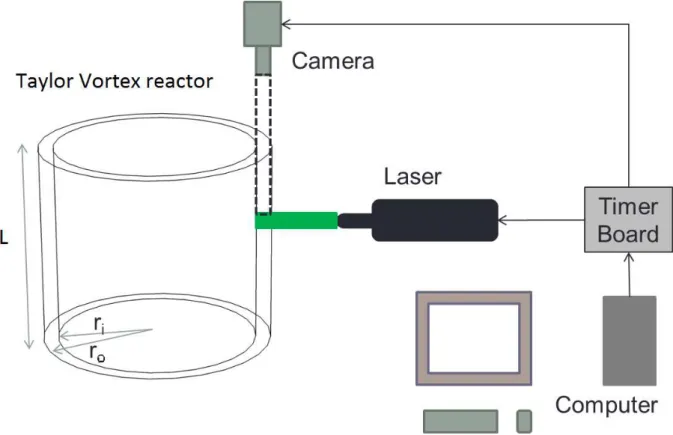
Figura 1 – Annual sales of recombinant proteins and monoclonal antibodies in the 2008-2013 period. Source: Ecker, Jones e Levine (2015). . . 31 Figura 2 – PIV system consisting of the TVB, laser, camera, synchronization

system and computer. . . 45 Figura 3 – Convergence statistics of moment of order one (a) and two (b) on a

horizontal plane located at ZL=0.725 and radially at Rb=0.082. . . 48

Figura 4 – Concentration of particles in a horizontal plane in the TVB at two diﬀerent rotational rates: 114 (the one behind) and 30 (the one in front) rpm without grid (a) and with a 32 square grid (b). . . 50 Figura 5 – Impact of particle size on the estimations of mean tangential velocity

(a) and squared ﬂuctuating velocity (b) for the horizontal plane located at Zh = 0.725± 0.005. . . 52

Figura 6 – Impact of time-step on the estimations of mean tangential velocity (a) and squared ﬂuctuating velocity (b) for the horizontal plane located at

Zh = 0.725± 0.005 using particle size of 20 µm. . . 54

Figura 7 – Influence of the time-step and particle size on the VEDR of mean flow kinetic energy.. . . 55 Figura 8 – Radial profile of mean tangential velocity at different overlap ratios and

ICS values at ZL = 0.725± 0.005. . . 56

Figura 9 – Radial profile of squared fluctuating tangential velocity at different overlap ratios and ICS values at ZL = 0.725± 0.005. . . 58

Figura 10 – Radial profile of the viscous dissipation of mean flow kinetic energy at different overlap ratios and ICS values at ZL = 0.725± 0.005. . . 59

Figura 11 – Radial profile of the viscous dissipation of mean flow kinetic energy at different overlap ratios and ICS values at ZL = 0.725± 0.005. . . 60

Figura 12 – Radial proﬁle of the viscous dissipation of turbulent kinetic energy at diﬀerent overlap ratios and ICS values at ZL = 0.725± 0.005. . . 61

Figura 13 – Figure no 20 of Tokgoz et al. (2012) presenting dissipation rate esti-mations for changing interrogation window sizes (IW) for Res=14,000

with exact counter-rotation of cylinders. 75 % overalap ratio was used for all IWs. . . 62 Figura 14 – Inﬂuence of the dimensionless spatial resolution of the maximum viscous

dissipation of turbulent kinetic energy estimated atZL = 0.725± 0.005

(15)

Figura 19 – The tangential (a) and radial b) velocity flow profiles at 30rpm. . . 68 Figura 20 – The total viscosity at different rotational speeds in the center of vortex

region. . . 71 Figura 21 – The evaluation of the constant C presented in the Equation 2.14. . . . 72 Figura 22 – The log-law proﬁle of the velocity in the center of vortex region of the

inner cylinder boundary layer. . . 73 Figura 23 – The tangential (a) and radial (b) normal stress profiles at 114 rpm. . . 74 Figura 24 – The tangential (a) and radial (b) normal stress profiles at 90 rpm. . . 75 Figura 25 – The tangential (a) and radial (b) normal stress profiles at 70 rpm. . . 76 Figura 26 – The tangential (a) and radial (b) normal stress profiles at 50 rpm. . . 77 Figura 27 – The tangential (a) and radial b) normal stress profiles at 30rpm. . . . 78 Figura 28 – The Reynolds shear stress,u′

ru

′

θ, proﬁles at 114rpm. . . 80

Figura 29 – The Reynolds shear stress,u′

ru

′

θ, proﬁles at 90 (a) and 70 (b) rpm. . . 81

Figura 30 – The Reynolds shear stress,u′

ru

′

θ, proﬁles at 50 (a) and 30 (b) rpm. . . 82

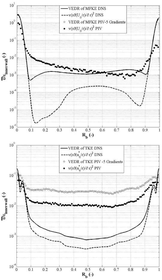
Figura 31 – The estimation of VEDR of mean ﬂow kinetic energy and its 5 gradients at ZL= 0.725 ±0.005. . . 83

Figura 32 – The estimation of VEDR of turbulent kinetic energy and its 5 gradients at ZL= 0.725 ±0.005. . . 84

Figura 33 – Comparison of isotropy assumptions on radial proﬁles atZL= 0.725 ±

0.005. . . 85 Figura 34 – Variation in the Kijkl ratios inﬂuenced by the dimensionless spatial

resolution for the radial proﬁles located at ZL= 0.725± 0.005. . . 86

Figura 35 – The VEDR of the mean ﬂow,ǫm, and turbulent, ǫt, kinetic energy at

114 rpm. . . 88 Figura 36 – The VEDR proﬁles of the mean ﬂow, ǫm, and turbulent, ǫt, kinetic

energy at 90 (a) and 70 (b) rpm. . . 89 Figura 37 – The VEDR proﬁles of the mean ﬂow, ǫm, and turbulent, ǫt, kinetic

energy at 50 (a) and 30 (b) rpm. . . 90 Figura 38 – The Kolmogorov scale for diﬀerent rotational speeds at the center of

vortex region. . . 93 Figura 39 – Geometry and mesh of the TVB used in the PIV experiments. . . 103 Figura 40 – Comparison of diﬀerent grid sizes for the DNS and LES models of

dimensionless mean axial velocity (a), radial velocity (b), tangential velocity (c) and mean square of ﬂuctuating tangential velocity (d) axially at Rb=0.067. The legend is same in all ﬁgures. . . 104

(16)

Figura 42 – Validation of the numerical DNS model with the PIV results of the log-law proﬁles for the tangential component at the inner (a) and outer (b) boundary layers. The κ = 0.4 and B = 5.2 is used in the log proﬁle. 108 Figura 43 – Validation of the numerical DNS model with the PIV results of

dimen-sionless mean squared ﬂuctuating tangential velocity component. . . . 109 Figura 44 – Validation of the numerical DNS model with the PIV results of the

VEDR of mean ﬂow (a) and turbulence (b) kinetic energy. . . 110 Figura 45 – Identiﬁcation of the Taylor’s vortexes through λ2 (a) and a pair of

secondary Taylor’s vortexes (b) for the DNS model. . . 116 Figura 46 – Identiﬁcation of the Taylor’s vortexes through λ2 for the LES-WALE

(a), and LES-Smagorinsky (b) models. . . 118 Figura 47 – Identiﬁcation of the Taylor’s vortexes through λ2 for the k-ǫ (a) and

RSM (b) models. . . 119 Figura 48 – Identiﬁcation of the Taylor’s vortexes through λ2 for the SST (a), and

SAS-SST (b) models. . . 120 Figura 49 – Radial proﬁles of the tangential velocity component near the outward

region of a Taylor vortex. . . 121 Figura 50 – Radial proﬁles of the tangential velocity component near the inward

region of a Taylor vortex. . . 121 Figura 51 – Radial proﬁles of the tangential velocity component near the center of

vortex region of a Taylor vortex.. . . 122 Figura 52 – Radial proﬁles of the radial velocity component near the outward region

of a Taylor vortex. . . 124 Figura 53 – Radial proﬁles of the radial velocity component near the inward region

of a Taylor vortex. . . 124 Figura 54 – Radial proﬁles of the radial velocity component near the center of vortex

region of a Taylor vortex. . . 125 Figura 55 – Radial proﬁles of the axial velocity component near the outward region

of a Taylor vortex. . . 126 Figura 56 – Radial proﬁles of the axial velocity component near the inward region

of a Taylor vortex. . . 126 Figura 57 – Radial proﬁles of the axial velocity component near the center of vortex

region of a Taylor vortex. . . 127 Figura 58 – Radial proﬁles of the log-law proﬁles of the axial mean of tangential

velocity component for the inner (a) and outer (b) walls for the different turbulence models. . . 128 Figura 59 – Radial profiles of the log-law profiles for the inner (a) and outer (b)

(17)

Figura 61 – Radial proﬁles of the tangential velocity component near the inward region of a Taylor vortex. . . 131 Figura 62 – Radial proﬁles of the tangential velocity component near the center of

region of a Taylor vortex. . . 135 Figura 69 – Radial proﬁles of the tangential velocity component near the outward

region of a Taylor vortex. . . 137 Figura 70 – Radial proﬁles of the tangential velocity component near the inward

region of a Taylor vortex. . . 138 Figura 71 – Radial proﬁles of the tangential velocity component near the center of

region of a Taylor vortex. . . 141 Figura 78 – Radial proﬁles of the turbulent kinetic energy near the outward region

(18)

Figura 79 – Radial proﬁles of the turbulent kinetic energy near the inward region of a Taylor vortex. . . 144 Figura 80 – Radial proﬁles of the turbulent kinetic energy near the center of vortex

region of a Taylor vortex. . . 144 Figura 81 – Comparison of the modeled turbulent kinetic energy with the one

estimated from the velocity data in the center of vortex region of a Taylor vortex. . . 145 Figura 82 – Presentation of anisotropy through Lumley-Newmann and AG graphs

axially near the walls, a) and b), and radially at the outward, center of vortex and inward regions of Taylor vortex, c) and d) respectively, for the DNS model. Note: in part a) and b) * represent the data near the inner and outer boundaries, while in c) and d) o, + and pentagram represent the outward, center of vortex and inward regions, respectively.147 Figura 83 – The twelve gradients of the VEDR of mean ﬂow (a) and turbulent (b)

kinetic energy for the DNS model. . . 149 Figura 84 – The estimation of the VEDR of mean ﬂow and turbulent kinetic energy

of the DNS model in the outward, center of vortex and inward regions . 150 Figura 85 – The Kolmogorov estimations of the DNS model calculated through the

VEDR of turbulent kinetic energy for the respective model and the mesh size. . . 152 Figura 86 – The estimation of the VEDR of TKE for the diﬀerent turbulence model

for axial mean of all the radial proﬁles. . . 153 Figura 87 – Three diﬀerent shapes of the outer bottom cylinder at 15 mm

oﬀ-bottom clearance and 1.968 _× 106_{, 2.24} _× ₁₀6 _{and 2.22} _× ₁₀6 _node

meshes, respectively, for each geometry. Green and purple markers signify interface area and periodic boundaries respectively. Please note that not all interface areas and periodic boundaries are shown here. . . 160 Figura 88 – Radial ﬂow proﬁles of the mean velocity for the mesh and time-step

independence study in the TVB with 5 mm oﬀ-bottom clearance and ﬂat bottom at ZL=0.57. . . 163

Figura 89 – Mean velocity comparisons between the sliding mesh and MRF techni-ques in the TVB with 5 mm oﬀ-bottom clearance and ﬂat bottom at

ZL=0.57. . . 164

Figura 90 – Comparison of numerical tangential velocity results with the PIV results of (COUFORT; BOUYER; LINE, 2005). . . 166 Figura 91 – Velocity and its three components in an axial proﬁle located at Rb=0.009.167

(19)

(20)

Lista de tabelas

Tabela 1 – Various parameters used to correlate to cell death in a Stirred tank. . 34 Tabela 2 – Dimensions and geometrical characteristics of the TVB used in the PIV

system. . . 44 Tabela 3 – Analytical estimations for the TVB used in the PIV system. . . 46 Tabela 4 – Diﬀerent ICS and overlap windows tested at ZL= 0.725± 0.005. . . . 47

Tabela 5 – Dimensionless Spatial resolution,δ/_hη_i, for diﬀerent rotational velocities, ICS values and overlap ratios located at ZL= 0.725± 0.005. . . 60

Tabela 6 – Mesh conﬁgurations used to model the TVB. . . 103 Tabela 7 – Torque and Power estimations in TVB through numerical and analytical

methods. . . 154 Tabela 8 – Dimensions and geometrical characteristics of the TVB used for studying

the different geometrical structures. . . 159 Tabela 9 – Grid independence study with the flat-bottom TVB at 5 mm off-bottom

clearance. . . 162 Tabela 10 – Mean percentage diﬀerence of the mean velocity between diﬀerent

meshes. . . 163 Tabela 11 – Analytical and numerical estimations of the Taylor reactor at 200 rpm. 173 Tabela 12 – Summary of VEDR and Kolmogorov micro-scales for diﬀerent

(21)

(22)

Lista de abreviaturas e siglas

CHO Chinese Hamster Ovary

CFD Computational Fluid Dynamics

DNS Direct Numerical Simulation

ICS Interogation Cell Size

LES Large Eddy Simulation

LDA Laser DopplerAnemometry

MFKE Mean Flow KineticEnergy

MRF Multiple Reference Frame

OBC Oﬀ BottomClearance

PIV ParticleImage Velocimetry

RANS Reynolds AveragedNavier Stokes

RMS Root Mean Square

RSM Reynolds Stress Model

(23)

SST Shear Stress Transport

TKE Turbulence Kinetic Energy

TVB Taylor Vortex Bioreactor

VEDR Viscous Energy Dissipation Rate

(24)

Lista de símbolos

b Gap width, ro - ri, m

bij Reynolds stress anisotropy tensor, m2s−2

d+ Radial coordinate at the inner wall, ruτ i/ν, (-)

C Constant of SAS-SST turbulence model, 2, (-)

C1ǫ Constant of k-ǫ model, 1.44 (-)

C2ǫ Constant of k-ǫ model, 1.92 (-)

C1ǫRSM Constant of LRR-IP RSM model, 1.45 (-)

C2ǫRSM Constant of LRR-IP RSM model, 1.9 (-)

C1RSM Constant of LRR-IP RSM model, 1.44 (-)

C2RSM Constant of LRR-IP RSM model, 1.92 (-)

Cµ Constant of k-ǫ model, 0.09 (-)

CS LES-Smagorinsky constant, 0.2 (-)

CS−RAN S Constant of LLR-RSM turbulence model, 0.22 (-)

(25)

F1 Blending function for the SST turbulence model, (-)

F2 Blending function for the SST turbulence model, (-)

Gk Generation of TKE for k-ǫ model, νtS2_, _m2_s−₃

k Turbulence kinetic energy, m2_s−₂

L Lenght of the outer cylinder, m

Lvk von Karmen length scale, (-)

obc Oﬀ-bottom clearance, m

p Pressure, Pa

p’ Modiﬁed pressure for RANS based two equation models, Pa

p” Modiﬁed pressure for RANS based RSM models, Pa

P Power, P = τ ω=RRR

v ρǫdv, Watts

r radial direction, m

ri Inner cylinder radius, m

ro Outer cylinder radius, m

(26)

Re Reynolds number, riω(ro−_r_i₎ ν , (-)

Sij Strain rate, s−₁

Ta Taylor number, r

1/2

i ω(ro−_r_i₎3/2 ν , (-)

u′_r Fluctuating radial velocity component,ms−₁

u′

θ Fluctuating tangential velocity component, ms −₁

u′_z Fluctuating axial velocity component, ms−₁

uτi Friction velocity at inner cylinder,ms−1

uτe Friction velocity at outer cylinder,ms−₁

Uθ Tangential component of the velocity, ms−1

Ur Radial component of the velocity, ms−₁

Utip Tip velocity, rω,ms−1

Uz Axial component of the velocity, ms−₁

v Volume of the reactor, m3

z Axial direction, m

ZL Dimensionless axial coordinate, _Lz, (-)

(27)

ǫinnerwall Mean viscous energy dissipation rate at inner wall,u4

τ/ν, m2s −₃

ηrr Radius ratio, ri ro, (-)

η Kolmogorov’s micro-scale, µm

δij kronecker delta, (-)

∆ local gird scale, m

κ von Kárman constant, (-)

Λ Taylors’s micro-scale, mm

λ1, λ2andλ3 Three eigenvalues of the vectorS2+ Ω2,s−2

ν Kinematic viscosity, m2_s−₁

νef f Modiﬁed kinematic viscosity of RANS based models, ν+νt, m2s−1

νsgs Subgrid scale eddy viscosity, m2_s−₁

νt Turbulent viscosity of RANS based models, m2_s−₁

η2 Constant of SAS-SST turbulence model, 3.51 (-)

Γ Aspect ratio, L_b, (-)

(28)

σk Constant of k-ǫ model, 1.0 (-)

σkSST Constant of SST turbulence model, 1/(F1/σk,1+ (1−F1)σk,2), (-)

σk,1 Constant of SST turbulence model, 1.176 (-)

σk,2 Constant of SST turbulence model, 1.0 (-)

σǫ Constant of k-ǫ model, 1.3 (-)

σǫRSM Constant of LRR-IP RSM model, 1.1 (-)

σωSST Constant of SST turbulence model, 1/(F1/σω,1+ (1−F1)σω,2), (-)

σω,1 Constant of SST turbulence model, 2.0 (-)

σω,2) Constant of SST turbulence model, 1.168 (-)

σΦ Constant of SAS-SST turbulence model, 2/3 (-)

βi,1 Constant of SST turbulence model, 0.075 (-)

βi,2 Constant of SST turbulence model, 0.828 (-)

β∗

∞ Constant of SST turbulence model, 0.09 (-)

τ Torque, Nm

τw Wall shear stress, N m−₂

(29)

ωtef turbulence eddy frequency of k-ω models, s−1

(30)

Sumário

1 INTRODUCTION . . . 31

1.1 Bioreactors and Hydrodynamics . . . 31

1.2 Understanding Hydrodynamics . . . 36

1.2.1 Experimental method . . . 37

1.2.2 Numerical method-CFD . . . 38

1.3 Overall project . . . 41

1.3.1 Main aim of this thesis . . . 42

2 EXPERIMENTAL METHOD - PIV . . . 43

2.1 Description of case set-up. . . 43

2.2 PIV set-up . . . 44

2.3 Estimation of VEDR . . . 47

2.4 Basic Aspects of PIV . . . 49

2.4.1 Concentration of particles . . . 49

2.4.2 Size of particles . . . 51

2.4.3 Time-step between frames . . . 53

2.4.4 Choosing overlap & ICS . . . 55

2.5 Results and discussion . . . 63

2.5.1 Mean velocity flow field. . . 63

2.5.2 Logarithmic velocity profiles . . . 69

2.5.3 Reynolds stresses . . . 72

2.5.3.1 Normal stress . . . 72

2.5.3.2 Shear Stress. . . 79

2.5.4 Viscous energy dissipation rate . . . 80

2.5.4.1 Composition of the VEDR . . . 80

2.5.4.2 EDR structure. . . 87

2.5.5 Kolmogorov scale . . . 92

2.6 Conclusions . . . 93

3 NUMERICAL METHOD AND ITS VALIDATION . . . 97

3.1 Turbulence modelling . . . 97

3.2 Numerical methodology . . . 102

3.2.1 Geometry and Meshing aspects. . . 102

3.2.2 Pre-processing aspects . . . 105

3.2.3 Solver & Post-processing aspects. . . 105

(31)

4 TURBULENCE MODELS . . . 115

4.1 Vortex identiﬁcation . . . 115

4.2 Mean velocity ﬂow ﬁeld . . . 117

4.2.1 Tangential velocity . . . 117

4.2.2 Radial velocity . . . 123

4.2.3 Axial velocity . . . 123

4.2.4 Log law profiles of tangential velocity . . . 125

4.3 Normal stresses . . . 129

4.4 Reynolds shear stresses . . . 137

4.5 Turbulent kinetic energy . . . 143

4.6 Anisotropy . . . 145

4.7 Viscous energy dissipation rate . . . 147

4.7.1 Composition of VEDR . . . 147

4.7.2 Structure of VEDR . . . 149

4.7.3 Power Estimation . . . 153

4.8 Conclusions . . . 154

5 AN APPLICATION OF CFD . . . 157

5.1 Problem description . . . 157

5.2 Computational model . . . 159

5.2.1 Description of case set-up . . . 159

5.2.2 Turbulence modeling . . . 161

5.2.3 Computational mesh and time-step . . . 161

5.2.4 Sliding mesh or MRF technique . . . 162

5.2.5 Computational aspects . . . 165

5.3 Validation of the computational model . . . 165

5.4 Results and discussion . . . 166

5.4.1 Mean velocity flow field. . . 166

5.4.2 Outer cylinder’s bottom shapes . . . 169

5.4.3 Off-bottom clearance . . . 170

5.4.4 Viscous energy dissipation rate(VEDR) . . . 172

5.5 Conclusions . . . 176

6 CONCLUSIONS . . . 179

(32)

APÊNDICE A – MATLAB FILE . . . 193

(33)

(34)

31

1 Introduction

1.1 Bioreactors and Hydrodynamics

The cultivation of animal cells (including human), a sub-area of biotechnology, in in vitro is a process of over 100 years old, but the emerging need of vaccines in the 1950s imparted some momentum to this process leading to the development of various vaccines such as measles (1963), rabies (1964), mumps (1967) and rubella (1969) (KRETZMER, 2002). In the mid-1970s, a second set of products hit the market - monoclonal antibodies by forming hybridomas from the fusion of cells, and genetic engineering (KRETZMER,2002).f Nowadays, the animal cell product list has increased to a huge number, namely, human and veterinary vaccines, diagnostics monoclonal antibodies and therapeutics, such as tPA, erythropoietin and interferons, with many animal cell products being highly costly in the order of US $ 104 _{to $ 10}9 _{per kilogram (KRETZMER,} _2002; _{ECKER; JONES; LEVINE,} 2015). The ever-increasing sales forecasts of the recombinant proteins and monoclonal antibodies till 2013 presented by Ecker, Jones e Levine (2015) can be seen in Figure 1, of which currently _≈ 54 % are being produced by animal cells (ECKER; JONES; LEVINE, 2015).

Figura 1 – Annual sales of recombinant proteins and monoclonal antibodies in the 2008-2013 period. Source: Ecker, Jones e Levine(2015).

(35)

culture media composition and process control, have resulted in over 100-fold yield increase in the cultivation of mammalian cells in the bioreactors for similar processes that were used in the mid-1980s (WURM, 2004). Nonetheless, there are still possibilities of further improvements in the yield through the optimization of various processes in the cultivation of animal cells (KRETZMER, 2002; WURM, 2004; JAIN; KUMAR, 2008; COSTA et al., 2010).

One of the most crucial factors that play a signiﬁcant role in the design of a bioreactor using animal cells is that they do not possess a cell wall, unlike bacteria, fungi and plant cells. Lack of cell wall makes the animal cells extremely sensitive to external environment such as pH, temperature, nutrients or culture media, regulatory molecules, oxygenation through bubbling and hydrodynamic forces resulting from aeration through bubbling and agitation in a bioreactor. These unique characteristics of animal cells makes it imperative to develop bioreactors designed with agitation and oxygenation systems that generate hydrodynamic forces milder than those found in bioreactors cultivating microbes (NIENOW, 2006).

Presently, the two most commonly employed bioreactors in large scale are the stirred or agitated tank and airlift reactor (CHU; ROBINSON, 2001; KRETZMER,2002; JAIN; KUMAR,2008;NIENOW,2006). From the 30 L in the 1960s to 8,000 L in 1980s to 20,000 L in the mid-2000s has been the increase in the capacity of a traditional agitated bioreactor to produce vaccines, monoclonal antibodies and therapeutics (NIENOW,2006; KRETZMER, 2002). On the other hand, the airlift bioreactor has been scaled up-to 2,000 L to produce monoclonal antibodies with reports of a 10,000 L airlift bioreactor which successfully cultured hybridoma cells to produce monoclonal antibodies (JAIN; KUMAR, 2008). Although, both bioreactor types have the versatility of cultivating both suspension and anchorage-dependent cells, the stirred tank has been the preferred choice of the industrialists due to easy scale-up, homogeneous environment and vast industrial experience of working with this reactor type (CHU; ROBINSON, 2001;NIENOW,2006).

(36)

1.1. Bioreactors and Hydrodynamics 33

to that of hollow ﬁber bioreactor.

In addition, in recent years, another reactor type, named Taylor-Vortex Bioreactor (TVB) has emerged as a choice for culturing cells (O’CONNOR et al., 2002; HAUT et al., 2003; CURRAN; BLACK, 2004; CURRAN; BLACK, 2005; GONG et al., 2006; TANZEGLOCK, 2008; SANTIAGO; GIORDANO; SUAZO, 2011; ZHU et al., 2010). These researchers successfully cultured various animal and insect cell lines, namely Chinese Hamster Ovaries (CHO), Human Embryonic Kidney, rat bone marrow stroma, and Sf-9 Spodoptera frugiperda, in suspension in a TVB. The oxygen is easily provided through gas-permeable membranes in these reactor types thus reducing the hydrodynamic stress due to aeration by bubbling (CURRAN; BLACK, 2005; SANTIAGO; GIORDANO; SUAZO, 2011). Another advantage of the TVB is the possibility of scale-up to an industrial level bioreactor, thus making it a serious contender for culturing animal cells (CHAUDHURI; AL-RUBEAI, 2005).

The design, scale-up and operation of bioreactors for animal cell culture require a comprehensive understanding of the mechanisms of cell damage and death caused by the fluid-mechanical forces associated with the equipment type (BRIONES; CHALMERS, 1994). Therefore, the parameters characterizing the effect of hydrodynamic forces causing cellular destruction are of crucial importance in the validation of bioprocess development studies conducted primarily in the mini-bioreactors and later transferred to the larger-scale bioreactors. Numerous parameters have been used to characterize cell death or damage in the various studies, as shown in Table 1, and a consensus has not been reached. Moreover, there is little information available on how to use flow parameters that correlate well with cell damage in one particular system to predict cell damage in a different system.

Briones e Chalmers (1994) stated that cell damage should ideally be predicted by knowing the actual stresses that the cell experiences, determined from intrinsic cell mechanical properties and the resulting cell deformation. Should the cell deformation exceed a critical value, the disruption of the cell structure would be expected. They suggested that the parameter chosen to correlate with cell damage should be 1) general in nature and not be dependent on the particular geometry and 2) be local, that is, not be averaged throughout the ﬂow domain.

(37)

Tabela 1 – Various parameters used to correlate to cell death in a Stirred tank. Cells used Range of

hydrodyna-mic Parameters Important Observati-ons Reference Insect Cells, SF-21

210- 510 rpm τ = 3 N/m2_{Cell death rate} proportional to volu-metric gas ﬂow rate

“Viability of cells de-creased at shear stres-ses of 1 N/m2_”

Tramper et al. (1986)

Hybridoma, CRl-8018

60-900 rpm, Cell de-ath correlates to Kol-mogorov eddy size si-milar to or smaller than the cell

“In absence of gas sparging, cells are da-maged only at speed above 700 rpm. No da-mage at speeds less than 600 rpm”

Kunas e

Papoutsakis (1990)

Hybridoma, HDP-1

100-440 rpm, Impeller tip speed 19-73.3 cm/s

“ Death rate constant, kd, increased sharply at impeller tip speeds above 40 cm/s”

Abu-Reesh e Kargi (1989) SF-9 and Hybridoma, serum con-taining, gas free

< 0.7 impeller tip speed, < 350 W/m3 Power Inputs

“Damaging threshold values of impeller tip speed or speciﬁc Power inputs for some animal cells”

Chisti (2001)

In the last 15 years, the group of Prof. Jeﬀrey Chalmers from the Ohio state university in USA have presented various meticulous studies of probably the ideal parameter to characterize the potential of hydrodynamic stresses to damage cells (GREGORIADES et al., 2000; MA; KOELLING; CHALMERS, 2002; MOLLET et al., 2004; MOLLET et al., 2007; MOLLET et al., 2008;GODOY-SILVA et al.,2009; GODOY-SILVA; MOLLET; CHALMERS, 2009).

(38)

1.1. Bioreactors and Hydrodynamics 35

ﬂow. Thus, the value of maximum turbulent VEDR that a cell can withstand would be substantially lower in a stirred tank than in a single-pass ﬂow device, since the integrated exposure time is considerably longer. Clearly, both the residence time of a single pass and the number of exposures to high turbulent VEDR in the vicinity of the impeller must be considered when estimating cell damage in a stirred-tank reactor, or any other type of bioreactor.

To overcome the limitation of single pass, the Chalmers group (GODOY-SILVA et al., 2009) presented a new method in which a microfluidic device is joined in an external loop to a 2 L stirred tank bioreactor. This way the cells were subjected to high VEDR levels multiple times, though there is no confirmation that the same cell was subjected to high VEDR levels of the microfluidic device multiple times. Nonetheless, similar high levels of maximum VEDR were reported having a lethal effect on the cells as reported by Ma, Koelling e Chalmers (2002). In addition, Godoy-Silva et al. (2009) also addressed another problem of the biological response of cells to sub-lethal levels of hydrodynamic stress. They found that the maximum VEDR for the sub-lethal effects is around 100 times smaller than the lethal dose. Sub-lethal levels are known to induce apoptosis in cells (ALOI; CHERRY, 1995), reduction in the production of the recombinant protein (GODOY-SILVA; MOLLET; CHALMERS,2009) and triggering the glycosylation shift of glicoproteins (GODOY-SILVA et al., 2009). Therefore, sub-lethal levels have to be taken into serious consideration to design a bioreactor with high productivity, reliability and operability for the cultivation of animal cells under strict guidelines implemented by regulatory agencies and required by the new cell lines.

(39)

systems. For instance, for a similar gas ﬂow rate of 4 L/m and rotational speed pf 700 rpm with similar concentration of oxygen in the air of 21 % in a stirred tank, the oxygen mass transfer rate for bubbling was 66.1 hr−₁

in comparison to the value for 3.3 hr−₁ for the gas-permeable membrane (SINGH, 2011).

Summarizing, it can be said that the choice of bioreactor depends upon the cell type, and the possibility of scale-up of the chosen reactor type. At the same time, an oxygenation method should be available with a priority of not creating additional hydrodynamic stress to the cell cultures in addition to the necessary evil of agitation to sustain homogeneous mixture in a reactor. Hence, the ease of scale-up, bubble-free oxygenation and proven capability of culturing various animal cells in suspension have lead to the TVB as the chosen reactor for this study. As a consequence, a detailed hydrodynamic study of this reactor type is a basic necessity in order to obtain the parameters which will guide towards the choice of optimum operating conditions with respect to high productivity and reliability.

1.2 Understanding Hydrodynamics

(40)

1.2. Understanding Hydrodynamics 37

1.2.1 Experimental method

Since early sixties, experimental methods have been shedding light on the flow structures and hydrodynamics in different fluid-flow configurations. In the early eighties and ninties, Smith e Townsend (1982) and Kobayashi et al. (1990) presented detailed experimental results of the mean and fluctuating velocities for a TVB using Pitot tubes and hot-wire anemometers. The biggest disadvantages of using these equipments were their intrusive nature and limited data in the boundary layers or near the walls in the case of TVB. Although, in recent years computational fluid dynamics (CFD) has become a more important tool for investigation, the experimental methods are still necessary in order to validate these numerical results. Mavros (2001) stated that among the various experimental techniques that are being practiced in recent years for flow visualization and analyzing hydrodynamics, particle image velocimetry (PIV) and laser Doppler anemometry (LDA) have become the predominant methods due to their relative easy-to-use techniques and non-intrusive nature. In the case of TVB, PIV has been the primarily used method (WERELEY; LUEPTOW, 1998; AKONUR; LUEPTOW,2003; COUFORT; BOUYER;

LINE, 2005;WANG; OLSEN; VIGIL, 2005; DUSTING; BALABANI,2009; DENG et al., 2010), to examine principally the velocity and vortex structures.

Hout e Katz(2011) andTokgoz et al.(2012) presented turbulence parameters, such as Reynolds stresses and VEDR, using the PIV method, but their spatial resolution was limited for turbulent Reynolds number. Due to limited spatial resolution, ranging from ﬁve to nine times the Kolmogorov scale, Hout e Katz (2011) observed severe underestimation as much as 55 % of the dissipation rate estimated assuming isotropy. Tokgoz et al. (2012) found that their tomographic PIV underestimated the mean dissipation, when comparing the PIV estimates with that of torque scaling, by 47 % and 97 % for shear Reynolds number of 3 800 and higher values, respectively. They worked with the spatial resolutions between 3 to 71 times that of Kolmogorov scale, thus also showing the importance of spatial resolution on the estimations of VEDR. In addition, they employed the large eddy PIV method, ﬁrst implemented by Sheng, Meng e Fox (2000) and demonstrated more than three times increase in the mean dissipation rate values.

(41)

Reaching a certain value of spatial resolution depends directly upon the chosen interrogation cell size (ICS) and overlap ratio, apart from the camera and lens equipment. Tokgoz et al. (2012) showed improvement in the estimation of VEDR with each decrease in the ICS, and increase in the overlap value at a particular ICS. However, there are various other factors, such as time-step between the double framed image, particle size and concentration, and higher orders of the ﬁrst derivative to estimate the gradients of the velocity vectors, which may also impact the VEDR. These aspects, as per author’s knowledge, have not been presented before.

Secondary problem with the PIV studies is that the spatial resolutions available for 3D is bigger compared to the 2D PIV studies. However, 2D PIV suﬀers from another limitation apart from the spatial resolution. For a direct estimation of VEDR from its equation (SHARP; ADRIAN, 2001), twelve gradients are required to be calculated, all of which can be estimated with a 3D PIV methods at the expense of spatial resolution. Whereas, in the case of 2D PIV methods only ﬁve gradients can be estimated. Due to this limitation, the rest of the seven gradients are required to be estimated based on the isotropic turbulence assumptions (SHARP; ADRIAN, 2001).

On the technological front, there has been a steady evolution in the equipments and the softwares used to interpret the images. The resolution of cameras has increased from 1 M pixels in late nineties to 16 M pixels in present time. The computer memory and disk space has also increased in order to capture and store such high resolution images, and their treatment to capture the smallest scales; for example, a set of 2500 double frame images of 16 MPixel camera is equivalent of 75 Gbytes and its treatment to resolve upto 25 µm is equivalent of 500 Gbytes. At the same time, the algorithms to estimate the correlation vectors have also improved and became more eﬃcient and reliable (STANISLAS et al.,2008).

One of the objectives of this study is to present a direct estimate of VEDR using a 2D PIV method, thereby presenting only ﬁve of the 12 gradients of a 3D equation of VEDR. The methods shown by Sharp e Adrian (2001) estimating the seven other gradients will also be included in this study. The 2D PIV method is used in order to capture the lowest possible spatial resolution with a 16 M pixel camera. A study will also be conducted to better understand the inﬂuence of not only the overlap ratio, and ICS but also the particle size and concentration, time-step and higher order gradients on the VEDR estimation.

1.2.2 Numerical method-CFD

(42)

1.2. Understanding Hydrodynamics 39

with 2D PIV estimations. In addition, significant recent advances in the computational field has enabled the researchers to use the direct numerical simulation (DNS) model to examine the hydrodynamics at high Reynolds number in a simple geometry, such as TVB. Understanding the hydrodynamics of a reactor are necessary for its optimization and characterization. In a TVB, consisting of two concentric cylinders, flow can be generated by rotating one or both cylinders in co- or counter-current directions. The field of study in such a reactor is the gap-width, the distance between the inner and outer cylinder, which is of the order of only few centimeters for laboratory scale reactors. As a result, obtaining a mesh which is nearer to the smallest Kolmogorov scale in order to capture around 90 % of the eddies is within reach. Indeed, there has been a surge in the studies of the TVB using the DNS model in recent years (BILSON; BREMHORST,2007; DONG, 2007;PIRRO; QUADRIO,2008;DOUAIRE, 2010;BRAUCKMANN; ECKHARDT, 2013).

Bilson e Bremhorst (2007) showed a detailed analysis of velocity fluctuations, turbulent kinetic energy (TKE), Reynolds stress budget and one-dimensional energy spectra for a radius ratio, η, of 0.617 and an aspect ratio, Γ, of 4.58. The main focus of the DNS study of Dong(2007) was to demonstrate the effect of the variation in Reynolds number on the Gortler vortices and herringbone-like streaks that develop near the cylinder walls, and partly the statistical features of turbulence in TVB. Pirro e Quadrio (2008) explained the numerical method that they developed extending the work of Quadrio e Lichini(2002) to use the DNS model in fully turbulent regime at Reynolds number of 10500. After validating with numerical and experimental results, they discussed mean velocity and root mean square value of velocity fluctuations profiles. Their major observation was the identification of two distinct sources of fluctuations, namely: 1) curvature related large-scale vortices, and 2) small scale fluctuations produced by the wall turbulence cycle. The objective of using the DNS model byDouaire(2010) was to be able to explain the cell behavior with respect to the TVB hydrodynamics at different Reynolds number. They used the DNS model to estimate various volumetric distributions, such as that of dissipation, and to follow the trajectories of a Lagrangian particle in order to find out the how much dissipation and force a particle faces in the reactor. More recently, Brauckmann e Eckhardt (2013) presented detailed torque estimations and how they are influenced by the vortex heights in TVB for a radius ratio, η, of 0.71 using DNS model at various aspect ratios and shear Reynolds number up to 3 _×104_.

(43)

known for their under-estimation of turbulence parameters (HARTMANN et al., 2004; DELAFOSSE et al.,2008). The LES model’s predictions of the turbulence quantities have been much better in the case of stirred tank (DERKSEN; AKKER, 1999; HARTMANN et al.,2004; DELAFOSSE et al.,2008) in comparison to the RANS based models. Though the mesh size used for the RANS model was much more courser in comparison to the mesh size used for the LES model (HARTMANN et al.,2004; DELAFOSSE et al., 2008), which could be one of the reasons behind the underestimation shown by the RANS based models. Study of Singh, Fletcher e J. (2011) in a stirred tank showed that improved mesh results in much better estimation of turbulence parameters by the RANS based models.

On the other hand, using the dynamic LES model in a TVB,Chung e Sung (2005) demonstrated a detailed validation of their numerical results, estimation of the anisotropy of the turbulent structures and probability density functions of the velocity fluctuations while focusing on the near-wall turbulent structures. Whereas, the aim of Oguic, Viazzo e Poncet(2013) was basically to validate their LES model based on their groups 2D compact fourth-order projection decomposition method presented by Abide e Viazzo (2005) and to present a brief study of anisotropy. Furthering on the research of Oguic, Viazzo e Poncet (2013),Friess, Poncet e Viazzo (2013) presented the LES-WALE (wall adapting local eddy) results of radial profiles of the rms velocities and the shear components of the Reynolds stress tensor along-with the axial and tangential velocity radial flow profiles. They also compared these LES-WALE results as a reference with a DES model and a RANS based RSM.

Considering these various studies, the objective of this study is to further the numerical research by: first, conducting a detailed validation of the DNS model with the 2D PIV estimations and; secondly, conducting a comprehensive comparison of different turbulence models for anisotropy, TKE and its terms, Reynolds stresses, and VEDR and its 12 terms in a TVB. In addition, a method on identification of vortex based on the study of Jeong e Hussain (1995) will be presented. Instead of the dynamic LES model, chosen by Chung e Sung (2005), the LES Smagorinsky and LES-WALE have been tested in this study. LES Smagorinsky has been the most commonly used LES model in case of stirred-tank reactor, though the impact of itsCS constant is also well known to have a significant effect on the turbulence quantities (DELAFOSSE et al., 2008). Based on the study of Delafosse et al.(2008), a value of 0.2 is chosen for the CS constant in this study. The LES-WALE model is chosen because of its better numerical stability and zero damping functions in near-wall treatment Friess, Poncet e Viazzo(2013); Moreover,Weickert et al. (2010) showed that it fared much better than the LES Smagorinsky model. The dynamic

(44)

1.3. Overall project 41

TVB in this study. The mesh used for these RANS based models will be the same that will be used in the case of DNS and LES models in order to have a much direct comparison between these models.

1.3 Overall project

Although, the stirred tank and the airlift reactor are being used in the industry currently for culturing animal cells in reactors of 20,000 L capacity, these reactors are limited to a select few cell lines which can be cultured in a suspension and which are comparatively less shear-sensitive. For newer, more shear sensitive cell line and those cell lines requiring microcarriers (a support matrix used in bioreactors on which the adherent cells are cultured) a different bioreactor is required which has the possibility of providing oxygen in liquid phase, in order to reduce the hydrodynamic stress, and which can provide a environment with low shear but homogeneous in nature for culturing of the animal cells. The TVB fits this bill perfectly, as oxygen can be provided in liquid phase easily and culturing of various animal cell-lines with and without microcarriers has been effective. Hence, the main aim of the overall project is to asses the possibility of using the TVB as a bioreactor for culturing shear-sensitive animal cells at an industrial scale. In order to see the effectiveness of the TVB as a bioreactor, a couple of its geometrical features will also be studied using CFD. As the overall project has a vast scope, it has been divided into different subgroups:

a) A detailed hydrodynamic study of the TVB and its geometrical features: as has been mentioned till now, a good understanding of hydrodynamics of a reactor are a must in order to put the animal cell death/injury in picture.

b) Scale-up study of the TVB with animal cell culture: the scale - up study will lay the base for the TVB to be projected as the future industrial scale reactor for culturing animal cells.

c) Feasibility of culturing of diﬀerent animal cell lines and a cell-line using micro-carriers.

d) A multiphase numerical study of the TVB in order to access the direct impact of hydrodynamics on microcarriers and animal cells in the same conditions in which they are being cultivated in the TVB.

(45)

1.3.1 Main aim of this thesis

As the overall project is beyond the reach of one thesis due to limited time and resources in order to understand this complex industrial problem, this thesis has been con-ducted with an aim to understand and present the hydrodynamics of the TVB with regards to its feasibility as a bioreactor for cultivating animal cell lines of biotechnological interest. The hydrodynamics of the TVB will be studied both experimentally and numerically with an aim to reach the smallest scales that are feasible based on the available ﬁnancial and technological resources. It is worth noting that the cost increases exponentially as we reach towards the smallest scales. Reaching the smallest scale is necessary for better estimation of the VEDR, which could be the ideal parameter to relate with the animal cell death (lethal impact) and/or injury (sub-lethal impact). Hence, the objectives of this thesis can

be described as:

a) Experimental study of the TVB with the aim of validating a numerical model while achieving the smallest feasible spatial resolution to obtain the VEDR estimations closest to the Kolmogorov micro-scale, and assessing the limitations of this 2D-PIV method.

b) Reaching the smallest scales require extra care, therefore, special attention will be given towards the basic aspects, such as overlap ratio, ICS, time-step and higher order gradients, of the PIV in order to ascertain their inﬂuence on the estimation of the VEDR among other parameters such as ﬂuctuating and mean velocity components.

c) The numerical study will be conducted with a CFD program named ANSYS-Fluent, and validated with the experimental results obtained with the PIV method.

d) Under the numerical methodology, the limitations and advantages of the diﬀerent turbulence models will be evaluated, and the chosen turbulence models will be used to study the hydrodynamics in detail, especially the VEDR.

(46)

43

2 Experimental Method - PIV

A 2D Particle Image Velocimetry (PIV) system measures instantaneous velocity flow in a plane. The in-house built computer software program or the one provided by the providers of the PIV system shows the vectorial velocity profiles in real time. The principal behind the measurement is the simple relation that velocity = distance /time. In this system, a sufficient amount of particles of very small size of _≈10-20 µm, are dispersed in the fluid assuming that these particles will follow the fluid movement. These particles are illuminated by a laser in a chosen plane in synchronization with a camera to capture a double frame image. The movement of particles between these two frames divided by the time-step between these two frames generates the velocity flow profile which can be extracted and treated further to estimate the fluctuating components and the VEDR.

2.1 Description of case set-up

Generally, a TVB, consisting of two concentric cylinders, is characterized on the basis of the rotation of one or both of the cylinders, resulting in the fluid motion due to the: 1) rotation of only the inner cylinder; 2) co-current rotation of both cylinders; and 3) counter-current rotation of both cylinders. Each of these types can be further characterized on the basis of the radius ratios of both cylinders and aspect ratio of the equipment. Radius ratio, ηrr, is the ratio of the inner cylinder radius, ri, to the outer cylinder radius, ro, or ηrr = ri/ro and aspect ratio, Γ, is the ratio of cylinder length, L, to gap width, b=ro₋ri, and Γ =L/b. In addition, Taylor number and Reynolds number also play a significant role in the classification of reactors in relation to the turbulence and vortex structures that will be present.

The Table 2presents the dimensions and geometrical characteristics of TVB used in the PIV study, as shown in the Figure 2. Water at room temperature was used as the working ﬂuid. The analytical estimations for these rotational speeds, shown in Table 3, were made using the (WENDT, 1933)’s correlation for estimating dimensionless torque-G shown in Equation 2.1, as mentioned by (LATHROP; FINEBERG; SWINNEY, 1992). These analytical estimations serve as the global estimates for this TVB conﬁguration.

G=

  

1.45 η3rr/2 (1−_η_rr₎7/4Re

1.5 _{f or4}_×₁₀2 _{< Re <}₁₀4 0.23 η3rr/2

(1−_η_rr₎7/4Re

(47)

Tabela 2 – Dimensions and geometrical characteristics of the TVB used in the PIV system.

Parameters Value (dimensions)

Inner cylinder radius, ri 100 (mm) Outer cylinder radius, ro 115 (mm) Length of the reactor, L 200 (mm) Gap width or distance between

in-ner and outer cylinder, b

15 (mm)

Oﬀ-bottom clearance(OBC) or the height at which inner cylinder is placed above the outer cylinder, c

0 (mm)

Radius ratio, η=ri

ro 0.87

Aspect ratio, Γ=h_b 13.3

Angular velocity, ω 3.14 to 11.94 (rad/s) Rotational speed, N 30 to 114 (rpm) Reynolds Nº, Re= riω(ro−r_i)

ν 4700 to17900

Taylors Nº, Ta= r

1/2

i ω(ro−ri) 3/2

ν 1825 to 6935

2.2 PIV set-up

The PIV system consists of a class IV Quantel Big Sky Laser (15 Hz andλ=532 nm), FlowSense EO 16 MPixel camera (4872_× 3248) provided by Dantec Dynamics using a 60mm objective having a diaphragm aperture of f/2.8 to f/32 and a synchronization system, shown in Figure 2. The black colored internal cylinder is made of PVC, and the transparent external cylinder is made of Plexiglas. The camera was placed on the top of the TVB to the capture the motion of particles in the X-Y plane. The XY plane is chosen in order to capture the radial ﬂow structures and radial gradients, which are assumed to be the principal components of the VEDR in a TVB. Capturing these smallest possible scales with regard to the radial gradients for a better estimation of VEDR is the main reason for the usage of the 2D PIV measurements in the X-Y plane, instead of the 3D stereographic or tomographic PIV study which would have provided the out-of-plane motion but at the expense of the spatial resolution.

(48)

2.2. PIV set-up 45

Figura 2 – PIV system consisting of the TVB, laser, camera, synchronization system and computer.

The focusing of the camera in the respective plane is the ﬁrst step of calibration, which was achieved by using a quarter-circular ﬂat plate of stainless steel with inner and outer radius one mm smaller than that of the inner and outer cylinders. The top of this plate was marked with horizontal and vertical lines one mm apart from each other forming a one mm square grid. The camera was focused on this plate and the images were saved in the computer program as calibration images. Then the second step for calibrating the images was conducted by computing a scale factor on the saved calibrated images. This scale factor was estimated by selecting two points on the saved images of the plate, and the known distance between the two points was provided. This procedure allowed the computer program to estimate the scale factor between the pixels and mm values along with the clarity of the images in that particular plane.

(49)

Tabela 3 – Analytical estimations for the TVB used in the PIV system.

Parameters Value (dimensions)

114 (rpm) 90 70 50 30

Moment, τ = Gρν2_{h, where} G = 0.23 η3rr/2

1−_η_rr 7/4

Re1.7_{, (WENDT,} 1933)

0.022 (Nm) 0.015 0.01 0.006 0.003

Angular Velocity, ω 11.9 (rad/s) 9.4 7.3 5.2 3.1

Tip Speed, riω 1.19 (m/s) 0.94 0.73 0.52 0.31

Wall shear stress at inner wall, τwi=τ /(2πr2

ih)

1.78 (N/m2₎ _1.19 _0.78 _0.46 _0.21

Wall shear stress at outer wall, τwo=τ /(2πr2

oh)

1.35 (N/m2₎ _0.9 _0.59 _0.35 _0.16

Friction velocity at inner wall, uτ i =qτwi/ρ

0.042 (m/s) 0.035 0.028 0.021 0.015

Friction velocity at outer wall, uτ o =

q

τwo/ρ

0.037 (m/s) 0.03 0.024 0.019 0.013

uτ i/riω 0.035 0.037 0.038 0.04 0.048

Global power, P=τ ω 0.27 (Watts) 0.14 0.07 0.03 0.01 Average VEDR, _hǫ_i=P/(ρπ(r2

o − r2

i)h)

0.132 (W/kg) 0.07 0.035 0.015 0.004

Average Kolmogorov’s micro-scale, hη_i= (ν3_/_h_ǫ_i₎1

4

52.5 (µm) 61.6 73.0 90.5 124.5

Average Taylor’s micro-scale, hΛ_i=q15νu2

i/hǫi

1.3 (mm) 1.4 1.5 1.7 1.9

VEDR at inner wall, ǫinnerwall = u4

τ i/ν

3.172 m2s−3

1.415 0.602 0.211 0.046

VEDR at outer wall, ǫouterwall = u4τ o/ν

1.814 m2_s−₃

0.809 0.344 0.121 0.027

the second order ﬂuctuating velocity components, namely u′2 r, u

′₂

θ andu

′

ru

′

θ, as shown in Figure3.

(50)

2.3. Estimation of VEDR 47

Tabela 4 – Diﬀerent ICS and overlap windows tested atZL= 0.725_± 0.005. ICS Overlap window Spatial resolution in µm

64 0 546

32 0 273 25 205 50 136 75 68 16 0 136 25 102 50 68 75 34

8 0 68

2.3 Estimation of VEDR

The PIV measurements were taken in a horizontal plan in a location where U or u’ = Uθ or u′

θ represents mean and ﬂuctuating tangential component and V or v’ = Ur or u′

r represents mean and ﬂuctuating radial component of the velocity. In this context, y represents the radial directions and θ = tan−₁

(y/x) represents the tangential direction, respectively, and were extracted as *.txt files from the image files using the Dantec Dynamic program Dynamicstudio V3.31. These txt files for the experimental results were treated with Matlab to create the gradients using the 2nd _{order central differencing approximation} of the first derivative, Equation 2.2, for the central elements. The boundary elements being only at the inner and outer wall due to the usage of the 2nd _{order scheme were not} considered for the VEDR estimation.

f_i′ = fi+1−fi−1

2h +E, E ∼= 1 6h

2₍

−f_i3) (2.2)

(51)

Figura 3 – Convergence statistics of moment of order one (a) and two (b) on a horizontal plane located at ZL=0.725 and radially at Rb=0.082.

shown in Equations2.5and2.6, respectively for the mean ﬂow and turbulence components.

ǫm =ν

   2   ∂Ur ∂r !2 + 1 r ∂Uθ ∂θ + Ur r !2 + ∂Uz ∂z

!2 + r

∂(Uθ/r) ∂r !2 + 1 r ∂Ur ∂θ !2 + 1 r ∂Uz ∂θ !2 + ∂Uz ∂r !2 + ∂Ur ∂z !2 + ∂Uθ ∂z !2

+2 ∂(Uθ/r)

(52)

2.4. Basic Aspects of PIV 49

ǫt=ν

     2    ∂u′ r ∂r !2 + 1 r ∂u′ θ ∂θ + u′ r r !2 + ∂u ′ z ∂z !2   + r

∂(u′ θ/r) ∂r !2 + 1 r ∂u′ r ∂θ !2 + 1 r ∂u′ z ∂θ !2 + ∂u ′ z ∂r !2 + ∂u ′ r ∂z !2 + ∂u ′ θ ∂z !2 +2   ∂(u′ θ/r) ∂r ∂u′ r ∂θ + 1 r ∂u′ θ ∂z ∂u′ z ∂θ + ∂u′ r ∂z ∂u′ z ∂r      (2.4)

ǫm =ν

 2   ∂Ur ∂r !2 + 1 r ∂Uθ ∂θ + Ur r

!2 + r

∂(Uθ/r) ∂r !2 + 1 r ∂Ur ∂θ !2

+ 2∂(Uθ/r)

∂r ∂Ur ∂θ   (2.5)

ǫt =ν

  2    ∂u′ r ∂r !2 + 1 r ∂u′ θ ∂θ + u′ r r !2   + r

∂(u′ θ/r) ∂r !2 + 1 r ∂u′ r ∂θ !2

+ 2∂(u

′ θ/r) ∂r ∂u′ r ∂θ   (2.6)

2.4 Basic Aspects of PIV

Every basic choice in the utilization of PIV equipment has a significant impact on the estimation of the finer quantities, such as VEDR. To estimate accurately the smaller structures a very fine spatial resolution is required. The interesting aspect is that the actual spatial resolution is known after the treatment of data, meaning that the concentration of particles, size of particles and time-step between frames is decided by hit and trail method. In addition, all these basic aspects are inter-related to each other. This section shows the importance of these basic aspects in the estimation of the VEDR. All these aspects were studied with the 114 rpm rotational speed unless otherwise stated.

2.4.1 Concentration of particles

(53)

sedimentation of particles with each decrease in the rotational speed from 114 rpm to 30 rpm. An improvement in the concentration may be required in order to attain a ﬁne spatial resolution as the rotational speed is decreased.

Figura 4 – Concentration of particles in a horizontal plane in the TVB at two diﬀerent rotational rates: 114 (the one behind) and 30 (the one in front) rpm without grid (a) and with a 32 square grid (b).