*e-mail: [email protected]
Two-Dimensional Control Volume Modeling of the Resin Infiltration of a
Porous Medium with a Heterogeneous Permeability Tensor
Jeferson Avila Souzaa*, Marcelo José Anghinoni Navaa,
Luiz Alberto Oliveira Rochaa, Sandro Campos Amicob
a
Departamento de Física, Universidade Federal do Rio Grande – FURG,
Av. Itália, Km 08 s/n, Campus Carreiros, 96201-900 Rio Grande - RS, Brazil
b
Departamento de Engenharia de Materiais,
Universidade Federal do Rio Grande do Sul – UFRGS,
Av. Bento Gonçalves, 9500, Campus do Vale, 91501-970 Porto Alegre - RS, Brazil
Received: December 21, 2007; Revised: April 22, 2008
Resin Transfer Molding (RTM) is a polymer composite processing technique widely used in the aeronautics and automotive sectors. This paper describes the numerical simulation of the RTM process where Darcy’s law was used for the mathematical formulation of the problem. A control volume finite element method was used for the determination of pressure gradients inside the mold, and a geometric reconstruction algorithm is used for the resin flow-front determination. Permeability of the medium was considered either a constant or a two dimensional tensor. The application was validated by direct comparison with literature data and good qualitative and quantitative agreement was obtained. The finite volume method was built to be used with a two-dimensional unstructured grid, hence allowing the analysis of complex geometries. The results showed that the proposed methodology is fully capable of predicting resin flow advancement in a multi-layer (with distinct physical properties) reinforced media.
Keywords: numerical simulation, resin transfer molding, finite volume method
1. Introduction
Composite materials have been widely used as an alternative material to metals. Many different techniques were developed for the molding of useful products. One of the most versatile technique is called Resin Transfer Molding (RTM). RTM is a very advantageous process compared to traditional techniques, because of the improve-ment in both performance and mechanical properties of the products. In addition, RTM is considered of low cost, able to produce more complex shapes with enhanced finishing of the parts, being largely employed in the automobile and aeronautics sectors. RTM has been used for different types of fiber reinforcements, comprised of either synthetic (e.g. carbon fibers) or natural (e.g. vegetable) fibers.
In RTM, a dry fibrous preform is placed into the mold. The mold is closed and a polymer resin is pumped from either a vacuum-assisted and/or an air-compressed-system into an injection gate at a specific location of the mold. Resin is expected to fill all the empty volume within the highly porous fiber reinforcement material1. Once the mold
is completely filled, a chemical cross-linking reaction (i.e. cure) oc-curs, allowing the material to achieve its specific properties in both micro and macro scales.
One of the earliest two-dimensional studies on infiltration of oriented fibers was reported by Bruschke & Advani2. Gebert3
estab-lished relationships between fiber volume fractions and permeability of oriented-fiber models in several angles. Endruweit and Ermanni4
used a fiberglass anisotropic preform as a two-dimensional model. Ac-cording to this model, the angle between fibers directly influences the filling time. Wang et al.5 simulated the permeability in a tissue plane
twisted non-homogeneously. He also studied how other parameters, e.g., density and fiber direction, affect permeability.
Another study published by Diallo et al.6 showed that resin flow
is directly influenced by the permeability in the transverse direction. These results were also validated by experimental data. Young et al.7
studied the flow into a multilayer preform and observed an important effect of the layer stacking sequence on the mold filling process.
Chen et al.8 employed the homogenization method to identify how
the micro-structure between layers affects the effective permeability of multilayer preforms. For that, their work was based on the hydrau-lic radius theory. Jinlian et al.9 performed numerical simulations of
flow-front for irregular filling using two simplified unit cells for in-plane impregnation of fabrics. Song & Youn10 presented an important
contribution by taking into account the through-the-thickness flow between adjacent layers, whereas Shojaei11 investigated the effect of
the type of fibrous material on the flow advancement and the final filling time.
One of the techniques for the numerical simulation of the resin transport through a porous media may be described following the determination of the pressure field and the consequent flow-front advancement. The pressure field is modeled with a Laplacian-like equation, which may be solved with a finite difference, finite element (most reported in the literature) or finite volume technique. For the flow front line advancement determination, a Flow Analysis Network (FAN) technique12 is normally used for RTM problems. This
without using remeshing schemes, therefore reducing the complexity, and usually the simulation time, of the numerical solution.
This work focuses on the fluid dynamics of the mold filling proc-ess and on the analysis of time and filling behavior. A computational tool was developed, which utilizes the finite volume method to cal-culate the pressure field within the mold and the FAN technique to determine the flow-front advancement of the resin. This methodology was also applied to solve problems where the medium is said to be orthotropic, that is, the permeability tensor has no null components on both x and y directions. Besides, this tool was validated by com-paring the numerical results with the analytical solution reported by Song & Youn10.
2. Resin Transport with Constant Permeability
Tensor
The problem addresses the modeling of resin transport through a fibrous reinforcement medium. The inner mold volume, which is to be impregnated with the resin, is considered a porous medium and the Darcy’s law formulation is used to determine the resin transport through the mold.
Experimental observations performed by Darcy showed that the fluid velocity through a column of porous material is proportional to the pressure gradient established along the column. The mathematical formulation for this phenomenon13 may be expressed as
1
( )
V= − K⋅ ∇P
µ
(1)
where V→ is the velocity vector (m/s), µ is the viscosity (Pa s), K= is the permeability tensor (m2) and ∇P is the pressure gradient (Pa).
The continuity equation for an incompressible fluid takes the form of
0 V
∇ ⋅ = (2)
combining Equations 1 and 2
1 .( K P)
∇ ⋅ ∇
µ (3)
For an isotropic medium and a Newtonian fluid (viscosity is as-sumed constant regardless of the shear rate),with constant physical properties, Equation 3 becomes
2P 0
∇ = (4)
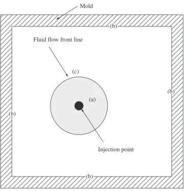
The flow of the resin or an ideal fluid (e.g. sunflower oil) in the RTM process is commonly simplified to Newtonian flow, due to the low and reasonably constant shear rate present throughout the flow. The boundary conditions to be used with Equation (3) are schemati-cally presented in Figure 1, being given by
a) P = P0 at the injection point;
b) P 0 n ∂ =
∂ at the mold walls (n is the direction normal to the
wall); and
c) P = Pf at the fluid flow-front, where Pf is the pre-set pressure at the flow-front.
The solution of Equation 3 inside the gray region of Figure 1 provides the pressure field gradient between the injection point and the region not yet impregnated with the resin, therefore the main goal of the simulation is to determine the fluid front position as a function of the injection time. Since Equation 3 does not include a transient term, the transient problem is solved by obtaining a steady state solution
for this equation for each time step. This solution consists of dividing the computational domain into a number of finite volumes, which are initially considered empty (without resin). Next, knowing the resin flow conditions of the previous time step (or the boundary condition at the first time step), the filling rate of the volumes adjacent to the flow-front is calculated and the time for filling these adjacent volumes can be estimated. Then, these newly filled volumes will compose a new flow-front for the resin inside the mold.
A preset pressure boundary condition (Pf) is set to the volumes at the flow-front and Equation 3 is again solved for the domain limited between the injection point (and walls) and the flow-front. The calculated pressure field is used to determine, with Equation 1, the resin velocity field. Then, the mass flow-rate passing through the control volumes can be calculated. This procedure is repeated until the mold is thoroughly filled.
The numerical solution of Equation 3 is obtained with a control volume finite element method14,15. The pressure field obtained by
solving Equation 3 is then used in Equation 1 for the determination of the resin velocity inside the mold. Since the numerical solution of Equation 3 is usually easily obtained, a significant part of the computational cost is spent on the determination of the advancement of the flow-front, which was obtained with a Flow Analysis Network (FAN) technique proposed by Frederick & Phelan12. First, the smallest
time-step needed to fill at least one volume is calculated by
( )
min ( )min
( ) f i i t t
t
∀ − ∀
∆ = ∀
(5)
where ∀i is the total volume of the finite volume i, ∀f
i (t) is the
filled volume at time t, and ∀- (t) is the volumetric flow-rate into volume i.
The (∆t)min is then used for the determination of the filling volume fraction and a filling factor f is defined as
(
)
( ) 1( )f
t i
i
t t
f t+ ∆ =t ∀ + ∆ ∀
∀
(6) Mold
Fluid flow front line
Injection point
(b) (b) (a) (c)
(b) (b) (b)
(b)
(b) (b)
Thus, this method is used to determine the resin flow-front posi-tion in dynamic problems of free-surface flow and has the advantage of using a fixed grid. The process is divided into two stages: flux calculation and flow front advancement. This procedure is maintained until complete mold filling12.
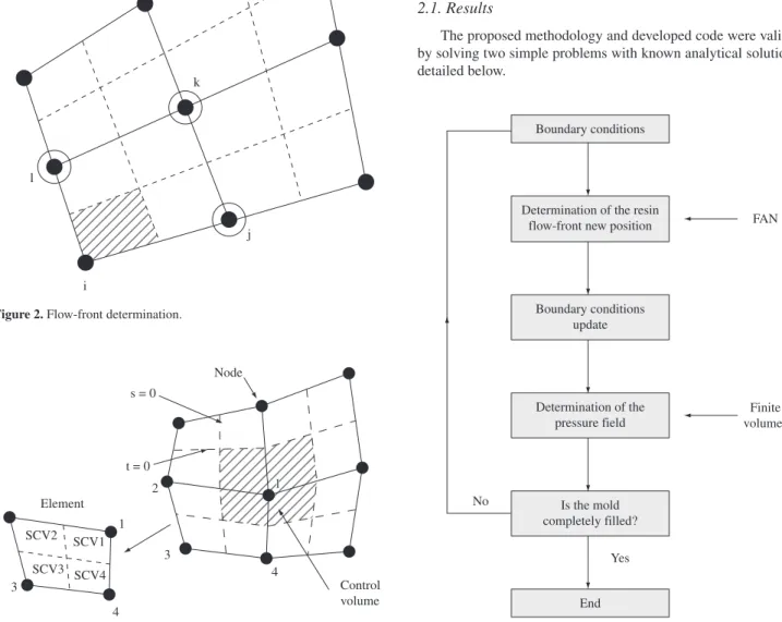
A point of the grid is considered to belong to the flow-front when at least one of the sub-volumes of that element shows a filling factor equal to one. For example, in the grid shown in Figure 2, the darkened sub-volume belongs to a fully filled control volume (f = 1), thus the points j, k and l are considered at the flow-front and a preset pressure boundary condition (P = Pf) is applied to them.
Figure 3 shows a control volume created around node 1 which is formed with the contribution of four sub-control volumes (SCV), each from a different element. The s and t variables represent the element local coordinates system. It can be observed in Figure 3 that the unstructured grid may be formed with irregular quadrilat-eral elements of different sizes, allowing the easy discretization of complex geometries.
The pressure field defined by Equation 3 does not have a closed (analytical) solution in the great majority of cases, thus a numerical procedure must be used for the solution of this equation. The meth-odology used in this work is very similar to that of well-known finite element/control volume-FE/CV methods, where the pressure field is obtained with a finite element solution of Equation 3. The calculated pressure field is then used in Equation 1 for the calculation of the velocity field and consequently the volumetric flow-rate through the control volume surfaces. Therefore, in the present work, the solution of Equation 3 is obtained with a finite volume method. This method14,15
defines on its basic formulation both the elements and the control volumes needed. The computational domain is discretized into ele-ments, each of them composed of four nodes (points) and the control volumes are created around the nodes with the contribution of four different elements. The flow passing by each volume is accounted for by integrating the balance equations (continuity and momentum) through the volume boundaries (surfaces).
Nodal filling factors are used for tracking resin flow-front ad-vancement. The filling factor for each node is defined as the control volume fraction filled by the fluid. Pressure is determined for com-pletely filled nodes and the comcom-pletely empty ones are ignored. The partially filled nodes are assumed to be close to the flow-front and the boundary conditions are then applied. The continuous update of the filling factors for each time step provides the flow-front position. Figure 4 presents the algorithm used for the numerical solution of the problem.
2.1. Results
The proposed methodology and developed code were validated by solving two simple problems with known analytical solution, as detailed below.
s = 0
t = 0
4
4 3
3 2
2
1
1 1 Element
Node
Control volume SCV2
SCV3 SCV4 SCV1
k
j
i l
Figure 2. Flow-front determination.
Figure 3. Control volume creation.
Determination of the resin flow-front new position
Boundary conditions
End Boundary conditions
update
Determination of the pressure field
Is the mold completely filled?
Yes No
Finite volumes
FAN
2.1.1. Rectilinear flow through a rectangular mold
Equation 5 was used to solve a simple porous media problem where a rectangular mold is boundary injected from the left side (see Figure 5a). This problem has a one dimensional behavior where the flow front should be a straight line that moves along the mold in the x direction. This is a simple problem which is very useful as a first test of the boundary conditions and the geometrical construction of the flow front. For a constant injection pressure condition, this problem has a analytical solution9 and the flow-front position x
f at a
time t can be calculated by13:
0
2 f
KP t x =
µ (7)
where P0 is the injection pressure (Pa) and t is the time of injec-tion (s).
The numerical solution was obtained with an 890-element grid and the flow-front position predicted by the model is in good quantita-tive agreement with the analytical solution, as shown in Figure 5b.
More refined grids where used for evaluating grid dependence, and the results were very close to the analytical solution, thus only one curve was plotted in Figure 5b.
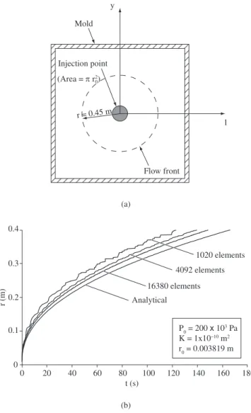
2.1.2. Radial flow from the center of a square mold
The second proposed problem is described in Figure 6a. In this problem, resin flow is obtained by applying a preset constant pres-sure P0 at the center of the mold. The resin will follow a radial flow pattern from the center towards the mold walls.
In this case, the relationship13 between the flow-front radial
posi-tion r and the injection time t is given by:
( )
2 2 2
0
0 0
1 ln
2 2
r
t r r r
KP r
µ
= − −
(8)
where r0 is the radius of the circular injection port.
A comparison between analytical and numerical solutions is shown in Figure 6b. One can observe that the solutions are initially very similar and that an accumulated error propagates with time, reaching a relative error of approximated 10% at r = 0.45 m. This error has already been reported in the literature16,17 and may be
reduced with grid refinement, as shown in Figure 6b for the 16,380 elements solution.
2.1.3. Case study
The developed application was used in the simulation of the resin flow-front advancement in a rectangular mold with an internal injection port located near the left wall (Figure 7a). A pressure P0 was preset at the injection port and the simulation was carried out until the complete filling of the mold. The medium and resin properties used are also shown in Figure 7a.
Figure 5. Boundary injection from one side of a rectangular mold: a) Problem sketch, and b) Analytical and numerical solution comparison.
Figure 6. Point injection (radial) from the center of a square mold: a) Problem sketch, and b) Analytical and numerical solution comparison.
y (m)
0.05
D 0.3
x (m) P0
Resin wall
P0 = 200 kPa K = 1 x 10⁻¹⁰ m²
= 0.01 Pa s
t (s) 0
0.00 0.05 0.10 0.15 0.20 0.25 0.30
3 6 9 12 15 18 21
xf
(m)
Numerical Analytical
r = 0.45 m
Injection point Mold
y
1
Flow front (Area = r2)
0
0.4
0.3
0.2
0.1
0
0 20 40 60 80 100 120 140 160 180
Analytical 16380 elements
4092 elements 1020 elements
t (s)
P0 = 200 x 10 3 Pa K = 1x10⁻¹⁰ m2 r0 = 0.003819 m
r (m)
(a) (a)
Figure 7b shows the flow-front advancement at different injec-tion times. It can be observed that the flow-front is somewhat radial at the beginning of the impregnation process, but assumes a one-dimensional aspect at x approximated equal to 0.12 m.
3. Resin Transport with a Heterogeneous
Permeability Tensor
In this section, the mathematical model was the same, however, a heterogeneous (orthotropic) permeability tensor was used, which may be described using its Cartesian components as
xx zz
K 0
K
0 K
=
(9)
where Kxx and Kzz are the permeability tensor components in the x and z direction (m2), respectively.
3.1. Results
3.1.1. Rectilinear resin transport through a multilayer
preform
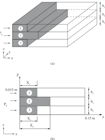
The problem under analysis has a preform divided into three orthotropic layers and rectilinear flow (injection from left to right). A two-dimensional model was assumed because the thickness do-main is much smaller than its length, as suggested by Shojaei11. Heat
transfer effects were not taken into account in the present work, i.e. isothermal flow was considered.
The XZ rectangular plane was evaluated. This plane enables the numerical analysis of the flow-front advancement in all preform layers in both x (length) and z direction (thickness). An injection
port, located throughout the thickness under analysis, was consid-ered, where a constant injection pressure P0 was preset. Figure 8a presents an isometric view of both mold and resin flowing within the three layers.
A slice of Figure 8a in the flow direction, with all the employed parameters, is presented in Figure 8b and Table 1, where h represents the layer thickness and ε is the porosity of each layer. For the simula-tions performed in this paper, the first and third layers were identical. A single resin (µ = 0.097 Pa s) is injected into the three layers, and permeability (Table 1) is the same for layers 1 and 3 and different (higher) for layer 2. In Figure 8b, x1, x2 and x3 represent the resin flow front position in each layer.
Song & Youn10 suggested an analytic solution for this type of
problem. The resin front position for each layer is given by
(
)
21
2 1
0 1 1
1 2
1 1 1 1 2
t
xx x x
P t K h K
x
h x h h x
−
= +
∈ µ + (10)
(a)
(a)
(b)
(b) 10 mm
77 mm
150 mm
300 mm
Injection gate
Mold
P0 = 200 x 10 3 Pa
K = 1 x 10¹⁰ m2
= 0.01 Pa s
0.1 s
0.1 s0.5 s0.5 s1 s1 s 3 s3 s 5 s5 s 10 s10 s 15 s15 s 20 s20 s
Injection area Injection area 0.15 m
0.075 m
0 0.05 m 0.10 m 0.15 m 0.20 m 0.25 m 0.30 m
Figure 7. Mold filling simulation: a) Problem sketch, and b) Flow-front at different injection times.
2 3
y
x z
h1
h2
h3
1 P0
x
x
z Z
h1
h2
h3
0.15 m 1
2
3 0.015 m
P0
X3
X2 X1
Figure 8. 3D representation of the rectangular mold showing resin flow within the preform10 a) and a transversal slice presenting the multilayer structure under analysis b).
Table 1. Fibrous preform properties.
Layer Kxx (m2) K zz (m
2) h (m) ε
Top (1) 12.4 x 10⁻¹⁰ 1.16
x 10–10 0.05 0.45
Middle (2) 57.8 x 10⁻¹⁰ 4.98 x 10⁻¹⁰ 0.05 0.45
Bottom (3) 12.4 x 10⁻¹⁰ 1.16
(
)
(
)
2 1 2 1 11 1 2 2
0
2 2
1 2 2 3
3
2 3 2
t
xx i
t
x x
K h k
x h h x
P t x
h x x
K
h h x
−
+ +
+
=
∈ µ −
+ (11) 3 3 2
0 3 3 2 3
3 2 3 2
3 3
( )
t xx
P t K h K x x
x
x h h x
h
−
= + +
∈ µ (12)
where xi is the resin flow-front position in each layer and t represents the time.
In addition, an average transversal permeability was defined, as follows 1 2 1 1 2 1 2 t zz zz h h K h h K K + = + (13) 2 3 3 3 2 2 3 t zz zz h h K h h K K + = + (14)
Figure 9 presents a comparison between the numerical results and those achieved analytically using Equations 10-12. Grid independ-ence, i.e. nearly the same solution for different number of elements, can also be verified in this figure.
In this work, a Control Volume Finite Element method for non-structured grids was employed to solve Equation 3. This alternative is quite useful to predict the extension of the fluid free surface located at the flow-front, since a single grid might be used (there is no need to recreate the grid at every time step). Besides, it is possible to simulate mold filling on a wide range of geometric shapes (even if highly complex).
As already stated, the 121 x 15 and 181 x 21 grid solutions in Figure 9 are nearly similar. This occurred because the analytical solu-tion (Equasolu-tions 10-12) takes into account only the mass transfer on the transversal direction (z axis) at the flow-front region of resin progress10.
Besides, a one-dimensional advancement for each layer (top, middle and bottom) of the flow is considered. On the other hand, the numerical solution descried in this paper does not have these simplifications.
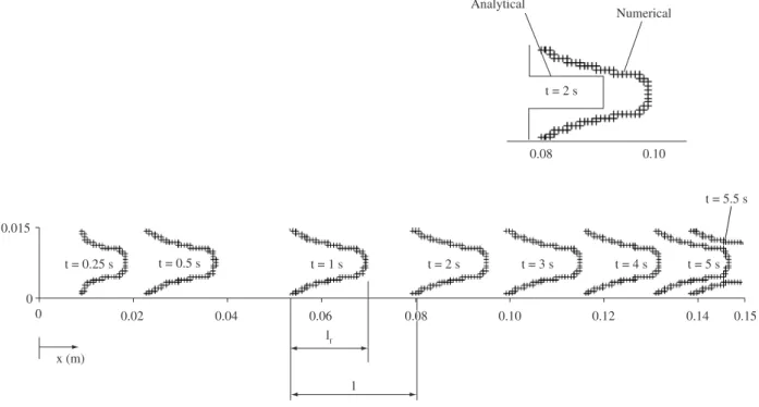
Figure 10 presents the resin position at several time steps. It can be verified that the distance l (distance between flow-fronts at different time steps) decreases with time. This is expected since the pressure is preset constant at the inlet, and therefore the gradient ∂P /∂x
de-creases with mold filling (i.e. due to an increase in x), consequently, decreasing flow velocity.
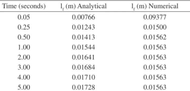
The distance lf (distance between the most advanced position of the flow-front and the least advanced one, at the same time step – see Figure 10), as calculated by the numerical and analytical solutions, is shown in Table 2. It can be seen that lf initially increases and later approaches a constant value in both methods.
Since the center region of the flow has a higher permeability, the fluid flows faster through that region. However, part of the resin volume is transferred transversally (called through-the-thickness flow) towards the mold walls, decreasing the flow velocity in that section. At the early stages of resin flow, both lf and through-the-thickness flow are mini-mum, allowing an initial quick development of the flow in the middle layer. After some time, the x direction flow in the least permeable layer combined with the through-the-thickness flow into this layer is found to be similar to the flow of the most permeable layer in the x direction, in a way that the distance between flow-fronts in both layers (with high and low permeabilities) tends to a constant value.
Figure 10 also presents a zoom of the flow-front in the 0.08 to 0.10 m region (filling time ≈ 2 seconds). It may again be observed that the numerical solution adequately represents the resin flow-front, whereas the analytical solution clearly simplifies it, with independ-ent advancemindepend-ents for each layer, what explains the small difference found in the solutions. Close examination of the observed velocity field in this region (Figure 11) confirms the direction of the resin flow transfer, from the middle layer towards the mold walls.
4. Conclusions
Although there are a few commercial softwares available world-wide to model the RTM process, a world-widely used technique to manufac-ture composites, Brazil still lacks research works on the basic analysis of the numerical methodology to simulate this process.
In this context, the main goal of this work is to report the prelimi-nary development of an application for the numerical simulation of the RTM process. A computational code using a finite volume method combined to a FAN technique has been developed for the simulation of the resin transport phenomenon.
Two problems with closed analytical solution were used for the validation of the code and the comparison between analytical and numerical solutions showed good qualitative and quantitative agree-ment, demonstrating the potential of the developed code to be used as a tool for the RTM process modeling.
In a more complex case, the porous media was considered an orthotropic fiber preform divided into three layers with different Kxx and Kzz permeability values. The comparison between the numerical model and a simplified analytical solution taken from the literature10
showed good qualitative agreement. The small difference between them was discussed based on the fact that the analytical solution 0.15
0.10
0.05
0
0 1 2 3 4 5 6
Analytical 61 x 9 volumes 121 x 15 volumes 181 x 21 volumes P0 = 60 x 103 Pa
= 0.097 Pa s
t (s)
Xf
(m)
Figure 9. Comparison between numerical and analytical solutions for the orthotropic case.
Table 2. lf values.
Time (seconds) lf (m) Analytical lf (m) Numerical
0.05 0.00766 0.09377
0.25 0.01243 0.01500
0.50 0.01413 0.01562
1.00 0.01544 0.01563
2.00 0.01641 0.01563
3.00 0.01684 0.01563
4.00 0.01710 0.01563
0.15 0.015
x (m)
0.04 0.06 0.12 0.14
0
0 0.02
t = 0.5 s
t = 0.25 s t = 3 s t = 4 s
t = 5.5 s
t = 5 s t = 2 s
t = 2 s
Numerical
0.10
0.10 0.08 Analytical
l t = 1 s
lf
0.08
0.08
Figure 10. Resin flow-front position with time and zoom at 2 seconds (top-right).
0.000 m
0.10 m 0.08 m
0.015 m
Figure 11. Detailed velocity field at a filling time of 2 seconds.
considers the through-the-thickness resin flow to take place only at the flow-front, but the developed model shows that a more complex velocity field is present and therefore yields a more precise description of the infiltration process in an orthotropic porous medium.
Acknowledgements
The authors are thankful to CAPES (PROCAD n° 0303054), FAPERGS (CASADINHO n° 0701263, PROADE 3 n° 05/2294.6) and CNPq for the financial support.
References
1. Um MK, Lee WI. A study on the mold filling process in resin transfer molding. PolymerEngineering and Science 1991; 31(11):765-771.
2. Bruschke MV, Advani SG. A finite element/control volume approach to mold filling in anisotropic porous media. Polymer Composites 1990; 11(6):398-405.
4. Endruweit A, Ermanni P. The in-plane permeability of sheared textiles. Experimental observations and a predictive conversion model. Composites A 2004; 35(4):439-451.
5. Wang Q, Maze B, Tafreshi HV, Pourdeyhimi B. A note on permeability simulation of multifilament woven fabrics. Chemical Engineering and Science 2006; 61(24):8085-8088.
6. Diallo ML, Gauvin R, Trochu F. Experimental analysis and simulation of flow through multilayer fiber reinforcements in liquid composite molding. Polymer Composites 1998; 19(3):246-256.
7. Young WB, Han K, Fong LH, Lee Lj, Liou MJ. Flow simulation in molds with preplaced fiber mats. Polymer Composites 1991; 12(6):391-403.
8. Chen ZR, Ye L, Liu HY. Effective permeabilities of multilayer fabric preforms in liquid composite moulding. Composites Structural 2004; 66(1-4):351-357.
9. Hu JL, Liu Y, Shao XM. Study on void formation in multi-layer woven fabric. Composites Part A: Applied Science and Manufacturing Composites 2004; 35(5):595-603.
10. Song YS, Youn JR. Flow advancement through multi-layered preform with sandwich structure. Composites A 2006; 38(4):1082-1088.
11. Shojaei A. A numerical study of filling process through multilayer preforms in resin injection/compression molding. Composites: Science and Technology 2006; 66(11-12):1546-1557.
12. Phelan FR. Simulation of the injection process in resin transfer molding. Polymer Composites 1997; 18(4):460-476.
13. Rudd CD, Long AC, Kendall KN, Mangin CGE. Liquid Moulding Technologies, SAE International. Warrendale, PA, USA: Woodhead Publishing Limited; 1997.
14. Souza JA, Maliska CR. Analysis of a volume based finite element methodology in view of the interpolation function employed and coupling characteristics. Proceedings of the Eighth Brazilian Congress of Engineering and Thermal Sciences-ENCIT; 2000 Oct 03-06; Porto Alegre, Brazil: ABCM; 2000.
15. Schneider GE, Raw MJ. Control volume finite-element method for heat-transfer and fluid-flow using colocated variables: 1. Computational procedure. Numerical Heat Transfer 1987; 11(4):363-390.
16. Dai FH, Zhang BM, Du SY. Analysis of upper- and lower-limits of fill time in resin transfer mold filling simulation. Journal of Composite Materials 2004; 38(13):1115-1136.
17. Joshi SC, Lam YC, Liu XL. Mass conservation in numerical simulation of resin flow. Composites A 2000; 31(10):1061-1068.
Nomenclature
f filling factor h layer thickness [m] K= permeability tensor [m2]
l length [m]
n normal direction P pressure [Pa] r radius [m]
V→ velocity vector [m s–1]
t time [s]
x flow-front position - Cartesian coordinate [m]
∀⋅ volumetric flow-rate [m3 s–1]
∀ volume [m3]
z Cartesian coordinate [m] Greek symbols
µ viscosity [Pa s]
ε porosity
Subscripts
f front line
min minimal
i volume index o injection section xx, zz tensor directions Superscripts