Phillips Curve in Brazil:
An Unobserved Components
Approach
♦Vicente da Gama Machado
Pesquisador - Banco Central do Brasil
Endereço: SBS - Quadra 3 - Bloco B - Edifício-Sede, Brasília/DF - Brasil CEP: 70074-900 - E-mail: [email protected]
Marcelo Savino Portugal
Professor - Universidade Federal do Rio Grande do Sul (UFRGS) Av. João Pessoa, 52 - sala 33 B - Porto Alegre/RS - Brasil CEP: 90040-000 - E-mail: [email protected]
Recebido em 14 de agosto de 2012. Aceito em 19 de março de 2014.
Abstract
This paper estimates reduced-form Phillips curves for Brazil with a framework of time series with unobserved components, in the spirit of Harvey (2011). However, we allow for expectations to play a key role using data from the Central Bank of Brazil’s Focus survey. Besides GDP, we also use industrial capacity utilization rate and IBC-Br index, as measures of economic activity. Our findings support the view that Brazilian inflation targeting has been successful in reducing the variance of both the seasonality and level of the inflation rate, at least until the beginning of the subprime crisis. Furthermore, inflation in Brazil seems to have responded gradually less to measures of economic activity in recent years. This provides some evidence of a flattening of the Phillips curve in Brazil, a trend previously shown by recent studies for other countries.
Keywords
New Keynesian Phillips curve, inflation, unobserved components
Resumo
Este artigo estima curvas de Phillips para o Brasil com uma abordagem de séries temporais com componentes não observados, seguindo Harvey (2011). Entretanto, é conferido um papel central a expectativas utilizando dados do Boletim Focus do Banco Central do Brasil. Além do PIB, empregamos a taxa de utilização da capacidade industrial e uma série ainda pouco explorada, IBC-Br, como medidas de atividade econômica. Os resultados apoiam a visão que o sistema de metas no Brasil tem sido bem-sucedido em reduzir a variância na sazonalidade e no nível da taxa de inflação, ao menos até o início da crise imobiliária americana. Além disso, a inflação parece ter respondido gradualmente menos a medidas de atividade no período recente. Tal fato constitui uma evidência de achatamento da Curva de Phillips no Brasil, tendência observada em estudos recentes de outros países.
Palavras-Chave
Curva de Phillips Novo-Keynesiana, inflação, componentes não observados
Classiicação JEL C32, E31
1. Introduction
The Phillips curve has unsurprisingly been a recurrent subject of debate in macroeconomics, since its formulation encompasses an important trade-off between inflation rate and unemployment rate or alternatively between inflation rate and output gap. Numerous countries use this aggregate supply relation when formulating and implementing monetary policy, often jointly with an aggregate de-mand equation (IS) and an interest rate rule. The Phillips curve is also frequently employed in inflation forecasting models, as reviewed by Stock and Watson (2008).
The focus of this study is to estimate alternative Phillips curves with unobserved components for the Brazilian economy, following to some extent the parsimonious approach proposed by Harvey (2011). A simple relationship is established between monthly inflation and output data, in which inflation is explained by a set of unobserved components (UC), in addition to the usual output gap and expected inflation terms. As a first step, output gap is identified by extrac-ting the cycle from the appropriate output series, also by the UC method.1
Differently from Harvey (2011), the inflation expectations term is explicitly introduced in the Phillips curve. Since we do not aim to impose rational expectations from the outset, we use data from the Central Bank of Brazil’s FOCUS survey, based on subjective expec-tations from a sample of firms. The stochastic trend component can be regarded as core inflation, substituting the lagged term of the hybrid NKPC. By adding the usual term corresponding to marginal cost, our model resembles a standard hybrid NKPC. Thereafter, a multivariate estimation is conducted, in which the appropriate ou-tput gap is implicitly present in the ouou-tput equation, instead of being inserted exogenously, which has the advantage of avoiding the pre-vious estimation of an additional unobserved component. Harvey’s “similar cycles” approach follows naturally since the cyclical move-ments of the two series are assumed to arise as a result of a common business cycle.
A secondary contribution concerns the use of output gap obtained from a trend-cycle decomposition of the Brazilian Central Bank’s index of economic activity (IBC-Br). Notwithstanding the relati-vely small sample size, interesting conclusions can be drawn from this series.2 We extend the model allowing for time variation of the output gap parameter, which is also new in comparison to Harvey
1 Some authors (Gali and Gertler, 1999 and Schwartzman, 2006 and Sachsida, Ribeiro and
Santos, 2009 in the Brazilian case) suggest that the output gap has not been a significant measure of inflationary pressures in GMM estimations. On the other hand, measures such as labour income share, or unit labor cost are also criticized for producing a countercyclical pattern in the analysis of U.S. data (Rudd and Whelan, 2007). As we introduce a different method for Brazilian series, we prefer to test the output gap, which is also an important policy variable for most central banks. However, capacity utilization rate and newly develo-ped IBC-Br series are also considered.
2 This index was adopted by the Central Bank of Brazil in 2009, in order to follow up
(2011). Some studies, as Kuttner and Robinson (2010), advocate a recent flattening of the Phillips curve in the US, in the sense that the output gap coefficient has become gradually smaller. This beha-viour has important macroeconomic implications, as we discuss later. Finally, an analysis of the forecasting power is carried out by compa-ring our models with a simple forecasting model in order to test the assumption that Phillips curves may provide good inflation forecasts (Stock; Watson, 2008).
This paper is organized into six sections. The next section briefly reviews existing literature. Section 3 deals with the econometric estimation of Phillips curves with exogenous marginal cost mea-sures, and the underlying conceptual issues. In section 4 we detail the multivariate estimation and its results, section 5 describes some extensions to the basic model, and Section 6 concludes.
2. Related Literature
Much of the literature that focuses on estimating the new Keynesian Phillips curve considers the inflation trend to be stationary, as re-viewed by Rudd and Whelan (2007) and Nason and Smith (2008b). On the other hand, recent works have sought to model Phillips cur-ves with a stochastic inflation trend, as done in the present study. Lee and Nelson (2007) propose a bivariate specification between inflation and unemployment, in which the inflation trend varies over time. Goodfriend and King (2009) explain the stochastic behaviour of inflation trend based on assumptions about central bank policy.
detail in Harvey (1989). However he does not consider inflation expectations, arguing that identification becomes difficult.
Our decision to use survey expectations directly in the estimations mirrors the seminal ideas from Roberts (1995), and more recently Adam and Padula (2011).3 The latter obtain significant estimates for the structural parameters once data from the Survey of Professional Forecasters are taken as proxy for expected inflation in the US.
With respect to the Brazilian literature on this issue, Sachsida, Ribeiro and Santos (2009) provide a good survey and propose a re-gime-switching model to account for time-variation in the Phillips curve parameters. Schwartzman (2006) estimates a Phillips curve using industrial capacity utilization data to address the fact that the output gap is not observable. Fasolo and Portugal (2004) adapt a NKPC for Brazil based on the NAIRU, emphasizing expectations formation. Arruda, Ferreira and Castelar (2008) and Correa and Minella (2005), used Phillips curve versions to assess their inflation forecasting power. To our knowledge, there are no Brazilian studies that investigate inflation dynamics with a primary focus on the de-composition of its factors into permanent and transitory unobserved components.
3. Basic Model with Unobserved Components
The main reference here is Harvey (2011), who used a structural time series approach with output gap as explanatory variable in a decomposition of the US inflation rate.
The specification with unobserved components has some advantages over ARMA models. First, the components here provide a straight-forward economic interpretation.
3 Among studies that used inflation expectations surveys, Basistha and Nelson (2007), for
But more importantly, in ARMA models, the dynamics relies ex-clusively upon the dependent variable, whereas in UC models, it is constantly inferred by observations.4
3.1. Comments on Harvey (2011) and our Divergences
Before moving on to the specification used, we make brief comments about Harvey’s (2011) model and about the adaptations performed.
A basic structural5 time series model of inflation can be easily re-presented by:
(1)
where the observed series πt is decomposed into trend (t), cycle (t), and seasonal (t) components, and into an irregular white noise component (1t). In addition to permanent and transitory compo-nents, it is possible to add explanatory variables, and also structural breaks, level breaks and outliers, as in a usual regression. The trend component in (1), augmented with cycles and seasonals, represents the underlying level of inflation.
Adding an output gap term ht to Equation (1), as a measure of infla-tionary pressure, the result is a Phillips curve similar equation, using unobserved components:
(2)
Harvey (2011) argues that, under some hypotheses, an inflation model with this configuration may simultaneously capture the backward- and forward-looking ideas of the hybrid new Keynesian
4 This point was made by Wongwachara and Minphimai (2009).
5 Models with unobserved components are also known in the literature as structural time
Phillips curve,6 which is notably based on lagged inflation, output gap and an inflation expectations component, like:7
(3)
In other words, Harvey (2011) focuses on estimating (2), assuming that this formulation contemplates the notion of a hybrid NKPC as in (3).
At least with respect to the lagged term, it is reasonable to affirm that it can be successfully replaced with the specification proposed here. It suffices to observe that a simple model that combines infla-tion and output gap ht:
(4)
can be written as:
(5)
where is an innovation and is a weighted average of past observations, corrected for the output gap’s effect. If we include cycle and/or seasonal components in (5), we have the term capturing both the past trend, and information on lagged inflation rates, appropriately weighted. This formulation seems to be more realistic than the Phillips curve with a plain lagged inflation term. In addition, as pointed out by Harvey (2011), admit-ting that ht is stationary in (4), the long-term inflation forecast is the current value of t, i.e., the unobserved term of the structural model becomes a measure of core inflation or underlying rate of inflation.
6 Gali and Gertler (1999) and Christiano, Eichenbaum and Evans (2005) are theoretical
references on the treatment of inflation through the hybrid new Keynesian Phillips curve.
7 Nason and Smith (2008b) argue that the hybrid NKPC is consistent with a variety of price
and information adjustment schemes. Therefore, the focus on reduced-form coefficients,b,
and f, instead of on structural parameters, simplifies the analysis without interfering in
In regard to the expectations term, our view diverge from that adop-ted by Harvey (2011), which assumed that the hybrid NKPC is equi-valent to an equation relating inflation to core inflation expectation, to expectation on the sum of future output gaps and to the current output gap, i.e.,
(6)
In addition to the need to appeal to several simplifying assumptions, this does not fully solve the problem, i.e., it does not allow, in gene-ral terms, modeling the past and future effects of hybrid NKPC as in the equation with unobserved components, or in the present mo-del, Equation (4). The author acknowledges the difficulty in doing so and places little importance on the future term, citing Rudd and Whelan (2007) and Nason and Smith (2008a).
Unlike Harvey (2011),8 we included an inflation expectations term in the analysis, as we consider it to be a crucial element when mo-deling inflation dynamics, in line with most of the new Keynesian literature. Furthermore, it is possible to check whether the futu-re term indeed plays a major role for Brazilian data in our model, as highlighted by Sachsida, Ribeiro and Santos (2009).9 However, Nason and Smith (2008b) draw attention to the weak identification of traditional GMM-based estimates of the NKPC. More impor-tantly, Orphanides and Williams (2005) point out that instrumental variables methods impose the unrealistic restrictions that monetary policy conduct and the formation of expectations are constant over time. These points further motivate the use of survey data in our study.10
8 Vogel (2008) also argues that inflation expectations should not be neglected in the basic
equation, while citing the difficulty in the identification of t in Harvey (2011) regarding
past or future effects.
9 According to their model, studies that consider the Phillips curve to be nonlinear
underesti-mate the role of the future term in the Brazilian inflation dynamics.
10 On the other hand, some authors highlight the drawback of survey-based forecasting bias, as
3.2. A Phillips Curve with Unobserved Components
The link between resource utilization and inflation is at the heart of the Phillips curve. Therefore, we begin by considering some real activity variable that represents the inflationary pressure (or the real marginal cost, as in the original NKPC). The most frequent exam-ples include labour income share, deviation from the natural rate of unemployment and the output gap. In the present study, the major focus is on the output gap, measured by two indicators of econo-mic activity, GDP and the IBC-Br series, which is published by the Central Bank of Brazil (BCB). It is expected that with the gradual and larger availability of data after the introduction of the inflation targeting system, the output gap may become more representative of inflationary pressures in Brazil.11 Additionally, we reproduce the same estimations with an indicator of monthly industrial capacity utilization rate (ICU) series.
A large strand of the literature is devoted to the estimation of the output gap series, which is not directly observed in the economy.12 Since the primary goal here is not to explore these techniques, we opted for decomposing the logarithm of output into unobserved trend and cycle components, as in Harvey (2011).
(7)
(8)
(9)
Simultaneously, we extracted the series seasonal component and stochastic cycle , which is equivalent to the output gap and takes on the following form:
(10)
11 This is true both for the IBC-Br series and for usual GDP series.
12 The main tools used in the applied literature are: production function approach, which has
where is a damping factor and in the frequency in radians . Error terms t and are normally independently distri-buted with variances and . and are mutually uncorrelated disturbances with zero mean and common variances . The dynamics of the stochastic seasonal component is identical with the one described next in Equations (14) and (15). Note that the expression above indicates a smooth trend which, together with a cyclical component, represents an attractive decomposition for ou-tput data, according to Koopman et al. (2007). The trend described in (8) and (9) can also be referred to as an integrated random walk. A traditional tool for trend extraction is the Hodrick-Prescott (HP) filter. However, even if the resulting output gap is similar to the one obtained here, the HP filter tends to be less efficient at the end of the series, as described by Mise, Kim and Newbold (2005).
Our estimations begin with a simpler Phillips curve (model I), adap-ted from Harvey (2011), with the inclusion of interventions in order to capture irregularities in the data:
(11)
where and follow the same dynamics of Equations (13) through (15).
Adding the expectations term, we obtain the proposed Phillips cur-ve model, which is classified as model II, III and IV in subsection 3.3, depending on the variable used as measure of marginal cost:
(12)
(13)
where each is generated by:
(15)
In the above expression for trigonometric seasonality, is the seasonal frequency in radians, and are normally indepen-dent distributed seasonal disturbances with zero mean and common variance . To choose the intervention dummy variables we analysed the auxiliary residuals, which are smooth estimates of the disturbances of irregular, level and slope components.13
Equation (12) is also called measurement or observation equation containing variables that explain the observed inflation. Equations (13) through (15) form the state equations that characterize the dynamics of unobserved variables. Note that inflation trend follows a local level approach, compatible with nonstationarity, which is com-mon in the literature. As to seasonality, component can be seen as the sum of time-varying trigonometric cycles.
For the implementation of the Kalman filter algorithm, it is neces-sary that the model’s equations are expressed in state-space form, i.e.:
In other words, our model basically resembles a reduced-form new Keynesian Phillips curve, with inflation expectations term and ou-tput gap as explanatory variables. Nevertheless, it also captures, to some extent, past inflation behaviour through the decomposed trend
13 The inclusion of the cyclical component
t was also tested, but it was found to incorrectly
and seasonality terms, in an attempt to mitigate an empirical defi-ciency that is commonly referred to in the literature.14
3.3. Data and Econometric Approach
Table 1 shows the series used to estimate Equations (11) through (15) as well as the multivariate analysis in section 4. Monthly GDP series at current prices, from April 2000 to May 2011 (source: http://www4.bcb.gov.br/?SERIESTEMP)was decomposed, following Equations (7) through (10), using the Kalman filter algorithm from the OxMetrics 5 package (STAMP module). The trend component obtained from the estimation is a good approximation for the po-tential output in the period. The difference between the observed series and its seasonally adjusted trend is the output gap. In this case, disregarding the error term, as its variance was very close to zero, we can easily assume that the cyclical component corresponds to the output gap. Similar reasoning was used to extract the output gap from the IBC-Br series.
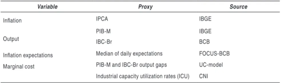
Table 1: Monthly data series
Variable Proxy Source
Inlation IPCA IBGE
Output
PIB-M IBGE
IBC-Br BCB
Inlation expectations Median of daily expectations FOCUS-BCB
Marginal cost PIB-M and IBC-Br output gaps UC-model Industrial capacity utilization rates (ICU) CNI
Notes: The IBC-Br series is only available after January 2003. IPCA: Broad consumer price index; IBGE: Brazilian Institute of Geography and Statistics; BCB: Brazilian Central Bank; PIB--M: Monthly output series built by interpolation of the quarterly series published by the BCB; IBC-Br: BCB´s Index of Economic Activity; CNI: Brazil’s National Confederation of Industry.
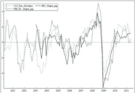
Figure 1 highlights the comparison of the series obtained from the PIB-M output gap, from the IBC-Br output gap and from relative deviations of the ICU, all of which are expressed as percentage.
14 Fuhrer and Moore (1995) were the first to argue that standard new Keynesian price
The percentage difference between actual ICU and its average for the period (calculated as 80.87%) was used to construct the devia-tions. Some clear patterns among all variables match the stylized facts in the Brazilian economy: first, a continuous economic activity growth period started in early 2006 and lasted until the first half of 2008; thereafter the subprime crisis caused a dramatic drop in ac-tivity. Second, a new period of economy growth apparently brought the observed output again above potential output and then more or less stabilized it over 2010. Inflation expectations were obtained from the Central Bank’s FOCUS survey. Here, we used the median of daily expectations within each month with respect to the next month.
First, we tested a model similar to the one used in Harvey (2011), which consists of equation (11) and is identified in Table 2 as model I. Then, to highlight the importance of introducing inflation expec-tations in the Phillips curve model with unobserved components, we use Equation (12) (Model II). In both alternatives, the measure of marginal cost used is the output gap calculated from the monthly GDP provided by the BCB (PIB-M).
The third model concerns a Phillips curve that is identical to (12), but with ICU data instead of output gap. Finally, model IV again consists of the same Equation (12), with the difference that the output gap series was calculated using IBC-Br series. The inclusion of interventions in important due to unusual inflation movements, especially around 2002 and 2003.
Model evaluation followed usual fitting and residuals diagnostic sta-tistics. With respect to fitting, the chief indicators contemplated in the estimation of the output gap and of the Phillips curve were the following: algorithm convergence, prediction error variance (PEV), and log-likelihood. According to Koopman et al. (2007), a good con-vergence is key to show that the model was properly formulated and has no fitting problems. Prediction error variance is the basic measure of goodness-of-fit which, in steady state, corresponds to the variance of the one-step-ahead forecast errors. Other diagnostic sta-tistics analysed include Box-Ljung’s Q stasta-tistics, for the assessment of residuals autocorrelation, and normality (N) and heteroskedasti-city (H) results.
3.4. Results
In the output gap estimation, a “very strong” convergence and a relatively small prediction error variance were obtained. The recent global financial crisis and the resulting sharp decrease in all econo-mic activity measures in the last quarter of 2008 and subsequent
recovery are noteworthy.
Table 2 summarizes key results from the different models described in Section 3.2. In all cases, convergence was again “very strong,” satisfying the main modeling criterion proposed by Koopman et al.
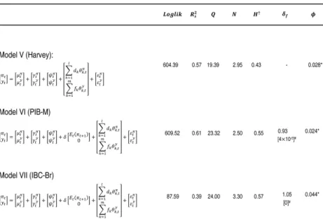
Table 2: Phillips curve estimation results
PEV Loglik Q N H f
Model I (Harvey) 0.052 143.43 0.54 29.310.04 0.56 - 0.017
[0.41]#
Model II 0.047 148.96 0.59 27.52 0.77 0.63 0.999 0.015
[3×10⁻⁵] [0.38]
Model III 0.047 148.87 0.59 30.32 0.90 0.63 0.995 0.009
[3×10⁻⁵] [0.66]
Model IV 0.029 117.97 0.45 26.163.46 0.58 1.08 0.034
[0] [0.001]
Source: Data obtained by the authors Notes: #Values in square brackets: p-value.
The interventions, in order of importance, and respective p-values for models I through III were as follows:
- Outlier in 2002/11. Model I: 1.35 [0]; model II: 1.26 [0]; model III: 1.27 [0]
- Level break in 2003/6: Model I: -0.74 [0.001]; model II: -1.01 [1×10⁻⁵]; model III: -1.02 [0]
- Outlier in 2003/9: Model I: 0.66 [2×10⁻⁴]; model II: 0.65 [1×10⁻⁴]; model III: 0.66 [1×10⁻⁴]
- Outlier in 2000/8: Model I: 0.94 [1×10⁻⁵]; model II: 0.81 [1×10⁻⁴]; model III: 0.82 [1×10⁻⁴]
- Outlier in 2000/7: Model I: 0.83 [1×10⁻⁴]; model II: 0.63 [0.003]; model III: 0.64 [0.002]
In model IV, the resulting interventions were: - Level break in 2003/3: -0.75 [0]
- Outlier in 2003/6: -1.25 [0] - Outlier in 2006/6: -0.36 [0.06].
As expected, the prediction error variance decreased from I to IV, indicating superior fit of the models that include inflation expec-tations (II through IV). Log-likelihood indicators underscore this conclusion, as they increased from I to III. In the case of model IV, the reduction is more a result of sample size than of the goodness of fit, given that log-likelihood is an absolute and cumulative indicator.
Again, the result is better for models II and III. According to Box-Ljung’s Q statistics, serial correlation of residuals is absent in all models and significance is lower than 0.1%.
With values lower than one, heteroskedasticity (H) tests indi-cate that the variance of residuals slightly decreases over time. Unequivocally, this results from the improvement of the inflation targeting regime in Brazil, with an increasingly larger convergence of the inflation rate towards the targets.
Even in model IV, with a more recent sample, the pattern signals at gradually lower variances. As to normality (N), the models clearly succeeded on the test, based on Doornik-Hansen’s statistic whose critical value at a 5% significance level is 5.99.
The slopes () of the different Phillips curve specifications – which are the coefficients for output gap and ICU deviation at the end of the sample – were positive in all cases, as theoretically expected, though not statistically significant in cases I to III. On the other hand, the output gap measure calculated based on the IBC-Br series was positively correlated with the inflation rate, with a high level of significance, although the amount of available data is smaller. The comment made by Tombini and Alves (2006), that smaller coeffi-cients than most of those described in the literature are due to the monthly frequency of data, applies here.
In regard to the coefficients of inflation expectations, the values showed high statistical significance and are close to one. Note that, although we do not impose long-run verticality of the Phillips curve, since the lagged inflation term is not made explicit, the results on
f suggest that such feature is present in the Brazilian economy, as
already showed by Tombini and Alves (2006) and other studies.
Test statistics particularly indicate a fitting improvement as we move from an approach without inflation expectations, as in Harvey (2011), to an approach that includes them. However, among models using output gap measures and the ICU deviations, there is no clear superiority, when it comes to fitting.
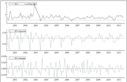
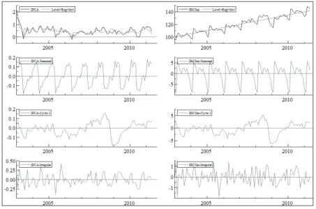
The first chart compares monthly observed inflation values (black line) with the decomposition into trend, regression and intervention effects (gray line). The middle chart shows seasonal effects. The figures correspond to the percentage contribution in price fluctua-tion due to seasonality. Note also that the variance of this effect decreases in more recent years, with a sharp increase in the effect in February and decrease in the effect in June over the last two years.
Finally, the lower graph shows the irregular component. Considering that the period between late 2002 and mid-2003 had the three most discrepant observations regarded as outliers, this chart also depicts some gradual reduction in the variability of disturbances.
Figure 2: Inflation decomposition - Model II
4. Multivariate Estimation
The joint specification of inflation and output differs from Harvey (2011) because of the introduction of the seasonal component and, especially, of the expectations term. Our main model is now:
(16)
where and represent the sets of outliers considered for the inflation and output series respectively.
The link between the series in the SUTSE approach is generally es-tablished by the correlations of errors of one or more components. Following Harvey (2011), we assume the cycles have the same au-tocorrelation function and spectrum. In other words, inflation and output cycles are modeled as “similar cycles”. In algebraic terms,
supposing ,
(
(
(17)
where and are 2 x 1 error vectors, such that , and is a 2 x 2 covariance matrix and . Figure 3 shows a joint plot of the cyclical components that were separately obtained from inflation and output, which gives a sense of inflation and out-put gaps. As in Harvey (2011), although they naturally have some correlation, thus justifying the similar cycles assumption, the two se-ries have a time-varying relationship, which calls for the UC model.
Figure 3 - Cycles obtained from univariate models for inflation and output (IBC-Br)
The cyclical component of inflation can be broken down into two independent parts, as follows:
(18)
where is a cyclical
compo-nent specific to inflation.
Thus, the inflation equation may be rewritten as:
(19)
In the bivariate case, three basic specifications are tested. Again, a similar approach to that of Harvey (2011) is compared with the model built above, in which one includes the future inflation ex-pectations term, as shown in Equation (16). They are represented as models V and VI. Finally, (16) through (19) are also employed considering the IBC-Br as proxy for yt (Model VII).
The relevant goodness-of-fit criterion in this case is a correlation matrix for the prediction error variance and the log-likelihood. We only show test diagnostics referring to the inflation equation in (16), since our main interest here is on Phillips curve estimations.
4.1. Results
Table 3 - Estimation results - bivariate case
Source: Data obtained by the authors
Notes: *The significance of parameter is not available as this parameter could only be indirectly estimated, as explained in (18) and (19).
#: Values in square brackets: p-value.
†: Statistics , Q, N and H refer only to the inflation equation.
The interventions considered in the inflation equation in models V and VI, in order of importan-ce, and the respective p-values were:
- Outlier in 2002/11. Model V: 1.41 [0] ; Model VI: 1.29 [0]
- Level break in 2003/6. Model V: -0.66 [6×10⁻⁴] ; Model VI: -0.87 [0]
- Outlier in 2003/9. Model V: 0.71 [3×10⁻⁴] ; Model VI: 0.67 [3×10⁻⁴]
- Outlier in 2000/8. Model V: 0.61 [0.005] ; Model VI: 0.56 [0.008]
In the output equation, level break in 2008/12. Model V: -0.09 [0]; Model VI: -0.09 [0]. In model VII, the resulting interventions were:
- Outlier in 2003/6: -1.16 [0]
- Level break in 2003/2: -0.74 [9×10⁻⁴]
- Outlier in 2003/9: 0.55 [0.005].
This illustrates the relatively calm pre-crisis setting in terms of mo-netary policy tensions, which was also in place in Brazil.
As to GDP, seasonal effects were reasonably constant in the sample. On the other hand, the cyclical component, which gives some no-tion about the output gap, showed a more erratic behaviour, with a sharpened drop at the end of 2008,15 due to the impact of the U.S. subprime crisis. Also, note how the modeling of similar cycles allo-wed for a contemporaneous pattern in both series coinciding with the crisis episode.
Figure 4 - Inflation and output (IBC-Br) – Bivariate model VII
Note: The IBC-Br is constructed based on the value of 100 in 2002. Inflation is expressed in monthly rates.
5. Extensions
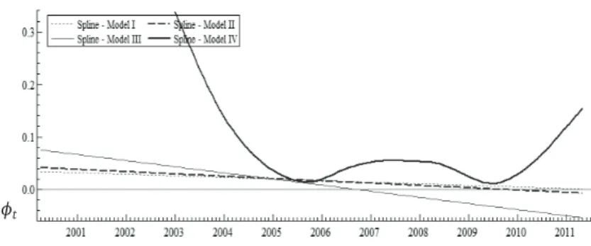
Two analyses were added to the basic models. The first one concerns the flattening of the Phillips curve, observed in studies for some developed countries. As shown by Kuttner and Robinson (2010),
15The behaviour of IBC-Br in late 2008 would also suggest a level break in trend, which
the parameter of Equation (12), which represents the response of the observed inflation to the output gap, has decreased in empirical analyses for the United States and Australia. A possible explanation is that, as inflation expectations become better anchored, the infla-tion response to supply shocks tends to be accommodated. An al-ternative justification states that the frequency of price-setting may depend on the average inflation rate, hence monetary policy could indirectly influence the slope of the Phillips curve, by lowering the inflation trend. As a first attempt to investigate whether the same occurs in Brazil, a variant of models I to IV was tested, in which the output gap coefficient was allowed to vary over time, i.e., we now have t, t = (Jan/2003,...,May/2011).
In this case, a smoothing spline was used, in which the slope of the Phillips curve varies according to:
(20)
The estimation of this new model is carried out with Equations (12) through (15) plus (20), which is an additional state equation.
Figure 5 - Dynamics of output gap coefficients in the Phillips Curve
The model finally assesses the forecasting power of a Phillips cur-ve model by comparing obsercur-ved inflation with the one calculated throughout the models, based on the minimization of one-step-ahead forecast errors. Stock and Watson (2008) reviewed Phillips curve based models in their ability to forecast inflation and obser-ved good performance in some cases. Nevertheless, Atkeson and Ohanian (2001) advocate that these forecasts tend to be worse than those based on simple univariate models. The widespread use of the NKPC in the literature and in actual policy therefore requires its forecasting power to be evaluated.16
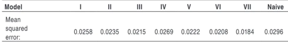
In the present study, the last 12 observations were excluded and the one-step-ahead inflation forecast was estimated for the period between April 2010 and March 2011. Mean squared error figures for each model are shown in Table 4.
Note that the models including inflation expectations had a higher forecasting power than Harvey’s variant, again corroborating the main argument of the present study. This occurred both in the uni-variate and biuni-variate cases. In the uniuni-variate specification, output gap extracted from IBC-Br was not very successful, but in the bivariate case, it yielded the lowest mean squared error among all estimations, despite its smaller number of observations.
16 Araujo and Guillen (2008) test the forecasting power of different Phillips curves based on
Table 4 - Mean squared forecast error – different specifications
Model I II III IV V VI VII Naive
Mean squared
error: 0.0258 0.0235 0.0215 0.0269 0.0222 0.0208 0.0184 0.0296
Source: Data collected by the authors
Forecasting power clearly increases in all cases when a multivariate specification is used. Finally, the mean squared error of a naive in-flation model was calculated. In such a model, expected inin-flation value is forecasted by its current value, i.e., . Our Phillips curve outperformed this specification, which corresponds to the last column.
6. Conclusions
Given the clear-cut empirical difficulties surrounding the Phillips Curve, the present study assessed inflation dynamics using an unob-served components approach for the Brazilian economy. By modi-fying Harvey’s (2011) approach, introducing an inflation expectation term in the Phillips curve, the model manages to parsimoniously express the dynamic relation between inflation and output gap. With the additional advantage of the graphical result, which allows a more direct economic interpretation of the components, we highlight the variability of the seasonal component of inflation, even within a sample of relatively few years. The relative reduction in this variabi-lity in the past years suggests that the inflation targeting system has contributed to reducing not only the inflation rates, but also their volatility within each year, at least until the subprime crisis effects came into place.
important for Brazilian monetary policy. Bivariate estimation clearly produced more attractive results and strengthened our results from the univariate estimation.
The analysis of the Phillips curve slope, represented by parame-ter t indicates a flattening Phillips curve in Brazil, as in Tombini and Alves (2006) and similarly to what is observed in developed countries, as reported by Kuttner and Robinson (2010). Finally, our model’s forecasting power was shown to outperform both a simple forecasting model and Harvey’s formulation, in terms of squared forecast errors.
Some issues could be subject of investigation of future research. For example, a comparison between the performance of output gap with that of other measures, such as unit labour cost or deviation from the natural rate of unemployment. One could also look at another approach that considers different dynamics of free and administered prices, and even possible distinctions between tradable and nontra-dable goods. Finally, comparisons to related countries using a similar approach could also prove useful.
References
ADAM, K.; PADULA, M. Inlation dynamics and subjective expectations in the United States. Economic Inquiry, v. 49, n. 1, p. 13-25, Jan. 2011.
ARAUJO, C. H.; GAGLIANONE, W. P. Survey-based inlation expectations in Brazil. In: BIS Papers.
Monetary policy and the measurement of inlation: prices, wages and expectations, Bank for
International Settlements, n. 49, p. 107-113, 2010.
ARAUJO, C. H.; GUILLEN, O. Previsão de inlação com incerteza do hiato do produto no Brasil. Anais do XXXVI Encontro Nacional de Economia, Salvador, 2008.
ARRUDA, E.; FERREIRA, R.; CASTELAR, I. Modelos lineares e não lineares da curva de Phillips para previsão da taxa de inlação no Brasil. Anais do XXXVI Encontro Nacional de Economia,
Salvador, 2008.
ATKESON, A.; OHANIAN, L. E. Are Phillips curves useful for forecasting inlation? Federal Reserve Bank of Minneapolis Quarterly Review, v. 25, n. 1, Winter 2001.
BASISTHA, A.; NELSON, C. R. New measures of the output gap based on the forward-looking New Keynesian Phillips curve. Journal of Monetary Economics, v. 54, n. 2, p. 498-511, Mar. 2007.
BONOMO, M. A.; BRITO, R. D. Regras monetárias e dinâmica macroeconômica no Brasil: Uma abordagem de expectativas racionais. Revista Brasileira de Economia, v. 56, n. 4, p. 551-589,
CALVO, G. Staggered pricing in a utility-maximizing framework. Journal of Monetary Economics, v.
12, n. 3, p. 383-398, Sept. 1983.
CHRISTIANO, L. J.; EICHENBAUM, M.; EVANS, C. L. Nominal rigidities and the dynamic effects of a shock to monetary policy. Journal of Political Economy, v. 113, n. 1, p. 1-45, 2005.
CORREA, A.; MINELLA, A. Mecanismos não lineares de repasse cambial: um modelo de curva de Phillips com threshold para o Brasil. Anais do XXXIII Encontro Nacional de Economia, Natal, 2005.
FASOLO, A. M.; PORTUGAL, M. S. Imperfect rationality and inlationary inertia: a new estimation of the Phillips curve for Brazil. Estudos Econômicos, São Paulo, v. 34, n. 4, p. 725-776, Oct./Dec. 2004.
FUHRER, J.; MOORE, G. Inlation persistence. Quarterly Journal of Economics, v. 110, n. 1, p. 127-159, 1995.
GALI, J.; GERTLER, M. Inlation dynamics: A structural econometric analysis. Journal of Monetary Economics, v. 44, n. 2, p. 195-222, Oct. 1999.
GOODFRIEND, M.; KING, R. G. The great inlation drift. NBER Working Paper Series, n. 14862,
Apr. 2009.
GORDON, R. J. The time-varying NAIRU and its implications for economic policy. Journal of Economic Perspectives, v. 11, n. 1, p. 11-32, 1997.
HARVEY, A. Forecasting, Structural Time Series Models and the Kalman Filter. Cambridge, UK:
Cambridge University Press, 1989.
______. Modelling the Phillips curve with unobserved components. Applied Financial Economics, v.
21, n. 1-2, p. 7-17, 2011.
HENZEL, S.; WOLLMERSHÄUSER, T. The New Keynesian Phillips curve and the role of expectations: Evidence from the CESifo World Economic Survey. Economic Modelling, v. 25, p. 811-832, 2008.
KOOPMAN, S. et al.STAMP 8: Structural Time Series Analyser, Modeller and Predictor. London:
Timberlake Consultants, 2007.
KUTTNER, K; ROBINSON, T. Understanding the lattening Phillips curve. The North American Journal of Economics and Finance, v. 21, n. 2, p. 110-125, Aug. 2010.
LEE, J.; NELSON, C. R. Expectation horizon and the Phillips curve: The solution to an empirical puzzle.
Journal of Applied Econometrics, v. 22, n. 1, p. 161-178, Jan./Feb. 2007.
MAVROEIDIS, S. Identiication issues in forward looking models estimated by GMM, with an applica-tion to the Phillips curve. Journal of Money Credit and Banking, v. 37, n. 3, p. 421-448, June 2005.
MISE, E.; KIM, T-H.; NEWBOLD, P. On suboptimality of the Hodrick-Prescott ilter at time series endpoints. Journal of Macroeconomics, v. 27, n. 1, p. 53-67, Mar. 2005.
NASON, J. M.; SMITH, G. W. Identifying the new Keynesian Phillips curve. Journal of Applied Econometrics, v. 23, n. 5, p. 525-551, Aug. 2008a.
______. The new Keynesian Phillips curve: Lessons from single-equation econometric estimation.
Federal Reserve Bank of RichmondEconomic Quarterly, v. 94, n. 4, p. 361-395, Fall 2008b.
PHILLIPS, A. W. The relation between unemployment and the rate of change of money wage rates in the United Kingdom, 1861-1957. Economica, v. 25, n. 100, p. 283-99, Nov. 1958.
ROBERTS, J. M. New Keynesian economics and the Phillips curve. Journal of Money, Credit and Banking, v. 27, n. 4, p. 975-984, Nov. 1995.
RUDD, J.; WHELAN, K. Modeling inlation dynamics: A critical review of recent research. Journal of Money, Credit and Banking, v. 39, n. 1, p. 155-170, Feb. 2007.
SACHSIDA, A.; RIBEIRO, M.; SANTOS, C. H. A curva de Phillips e a experiência brasileira. Textos
para Discussão IPEA, Brasília, n. 1429, out. 2009.
SCHWARTZMAN, F. F. Estimativa de curva de Phillips para o Brasil com preços desagregados. Eco-nomia Aplicada, Ribeirão Preto, v. 10, n. 1, p. 137-155, jan./mar. 2006.
STOCK, J. H.; WATSON, M. W. Phillips curve inlation forecasts. NBER Working Paper Series, n.
14322, Sept. 2008.
TOMBINI, A. A.; ALVES, S. A. L. The recent Brazilian disinlation process and costs. BCB Working Paper Series, Banco Central do Brasil, n. 109, June 2006.
VOGEL, L. The relationship between the hybrid new Keynesian Phillips curve and the NAIRU over time. Macroeconomics and Finance Series, Hamburg University, n. 3, Oct. 2008.
WONGWACHARA, W.; MINPHIMAI, A. Unobserved components models of the Phillips relation in the ASEAN Economy. Journal of Economics and Management. v. 5, n. 2, p. 241-256, 2009.
WOODFORD, M. Interest and Prices: Foundations of a Theory of Monetary Policy. Princeton: