M
ASTER
I
NTERNATIONAL
E
CONOMICS AND
E
UROPEAN
S
TUDIES
M
ASTER
´
S
F
INAL
W
ORK
D
ISSERTATION
T
HE
2000
AND
2014
S
UPPLIERS AND
U
SERS
N
ETWORKS
:
A
N
ETWORK
A
NALYSIS OF
T
RADE IN
V
ALUE
A
DDED
S
USANA
R
ITA
C
OELHO
V
IEIRA
O
CTOBER
-
2018
2
M
ASTER
INTERNATIONAL ECONOMICS AND EUROPEAN
S
TUDIES
M
ASTER
´
S
F
INAL
W
ORK
D
ISSERTATION
T
HE
2000
AND
2014
S
UPPLIERS AND
U
SERS
N
ETWORKS
:
A
N
ETWORK
A
NALYSIS OF
T
RADE IN
V
ALUE
A
DDED
S
USANA
R
ITA
C
OELHO
V
IEIRA
S
UPERVISION
:
M
ARIA
P
AULA
F
ONTOURA
O
CTOBER
-
2018
3 Abstract
The present work provides a theoretical contribution to the relevance of the network analysis method to analyse the world’s suppliers and users networks. It inserts itself in a stream of studies that consider that Input Output (IO) matrixes are in itself weighted and directed networks accounting for different values of supply-use flows between countries and sectors.
Global Value Chains represent the breakup of production in several stages, each taking place in a different country. In this context, traditional statistics do not fully capture the fragmentation of international production, being responsible for double counting in import and export data. To fill this gap, a handful of internationally linked IO datasets have emerged. Rather than simply trusting in a commodity or service classification, the focus of those datasets is in supply-use relationships.
Several international economists and econophysicists have advocated the potential of the network analysis method to the analysis and visualisation of the trade networks, however, the use of trade statistics leads to incomplete conclusions. Therefore, a relatively recent body of literature has applied network analysis in the study of GVCs. The differences between both approaches are not only in the type of issues studied but also in the conclusions.
This work makes use of the network analysis method to characterize the evolution of the world’s trade in value added between 2000 and 2014. It uses data from the latest release of the WIOD database to build trade in value added indicators that will be later used for graph visualization and for computation and analysis of three network based-measures. In contrast with previous studies, it includes more recent time moments, consolidating of some of the previous conclusions. In line with previous studies, we conclude that only a small number of occupy central positions in the production networks. This condition is verifiable either in the number of partners, in the value of bilateral supply and/or use relationships and in the connections with other central partners.
Keywords: Global Value Chains; Input-Output Matrix; Trade in Value Added;
4 Resumo
O presente trabalho constitui uma contribuição teórica para a discussão da relevância do método de análise de redes na análise da rede mundial de fornecedores e utilizadores. Insere-se numa corrente de estudos que considera que as matrizes Input-Output (IO) são por si só redes ponderadas e direcionadas que contém diferentes valores de fluxos abastecimento/uso entre países e sectores.
As Cadeias Globais de Valor (CVG) representam a fragmentação da produção em várias fases, cada uma localizada num país diferente. Neste contexto, as estatísticas tradicionais de comércio não refletem a fragmentação da produção internacional, sendo responsáveis pela dupla-contagem nos dados de importações e exportações. Para preencher esta lacuna, surgiram bases de dados IO com links internacionais, estas bases de dados são baseadas em relações de abastecimento e uso em detrimento da simples classificação de bens e serviços.
Vários economistas internacionais e econofísicos defendem o potencial da análise de redes para a análise e visualização de redes de comércio, contudo, a utilização de estatísticas tradicionais de comércio compromete os resultados. Mais recentemente, um número significante de trabalhos tem utilizado o método da análise de redes no estudo das CGV. As abordagens diferem no tipo de problemáticas estudadas e nas conclusões. O presente trabalho utiliza o método de análise de redes para caracterizar a evolução do comércio de valor acrescentado mundial entre 2000 e 2014. Os dados, da base de dados WIOD (2016), são primeiramente utilizados para a criação de indicadores de comércio de valor acrescentado que serão posteriormente utilizados para a visualização dos grafos e para o cálculo e análise de três medidas de análise de redes.
Em contraste com estudos anteriores, este trabalho inclui momentos temporais mais recentes, permitindo a consolidação de resultados anteriores. Em consonância com estudos anteriores, conclui-se que somente um pequeno número de países ocupa posições centrais nas redes de produção mundiais. Esta condição verifica-se quer no número de parceiros, valor das relações bilaterais e na conexão com outros parceiros mais centrais.
Palavras-chave: Cadeias Globais de Valor; Matriz Input-Output; Comércio de Valor
5 Agradecimentos
À minha orientadora, Professora Doutora Maria Paula Fontoura pela disponibilidade, confiança e por ter colocado a fasquia sempre um pouco mais alta.
Aos membros do júri, Professor Doutor Renato Flôres Jr. e Professor Doutor António Augusto Mendonça pelas valiosas sugestões que contribuíram para o melhoramento deste trabalho.
A todos aqueles que, ao longo dos anos, foram cruzando o meu caminho e que pelas experiências partilhadas e palavras trocadas me incentivaram a cultivar um espírito crítico e constante curiosidade.
À minha família mais próxima pelo afeto, preocupação e confiança. Aos meus pais e irmã por tudo o resto, que é a maior parte.
6 Acronyms
BRIICS - Brazil, Russia, India, Indonesia, South Africa DVA - Domestic Value Added
EC - Eigenvector Centrality FVA - Foreign Value Added GVCs - Global Value Chains
ICTs - Information and Communication Technologies IO - Input-Output
ITN - International Trade Network
NAFTA - North Atlantic Free Trade Agreement ND - Node Degree
NS - Node Strength
OECD - Organisation for Economic Cooperation and Development OECD ICIO - OECD Inter-Country Input-Output
RoW - Rest of the World TiVA - Trade in Value Added
TTVA – Total Trade in Value Added VS - Vertical Specialisation
WIOD - World Input-Output Database WTN - World Trade Network
WTO - World Trade Organisation WTW - World Trade Web
7 Table of Contents
1. Introduction 8
2. Measures of Trade in Value Added 10
3. Measuring Trade in Value Added for Countries in 2000 and 2014 15
4. World Trade Networks – Network analysis with traditional trade statistics 18
5. Networks of trade in value added – Network analysis with input-output trade statistics22
6. The world users and suppliers network (2000 and 2014) 25
7. Network visualisation and network-based measures 27
8. Final Remarks 36
References 37
Annexes 40
Annex 1 - Total Node Degree and Node Degree Strenght, 2000 and 2014 40 Annex 2 – Node Strenght Percent Rank Analysis 42
Annex 3 – Eigenvector centrality results 44
Annex 5 – Tecnhical Appendix 48
Annex 6 – Countries’ Abbreviations in WIOD Database 49 Figures Index
Figure I: Decomposition of Gross Exports and the various streams of literature ... 13
Figure II: Gross exports and Value Added Trade measures from the perspective of a 2 country, 2 sectors internationally linked IO database ... 14
Figure III: Main branches of literature for network analysis in trade and in TiVA ... 24
Figure IV: The world’s users and suppliers network, 2000 ... 26
Figure V: The world’s users and suppliers network, 2014 ... 27
Figure VI: Total node degree distribution 2000 and 2014 ... 31
Figure VII: Total node strengh distribution 2000 and 2014 ... 31
Figure VIII: Eigenvector centrality distribution 2000 and 2014 ... 33
Tables Index Table I: Trade in value added measures for WIOD 43 countries and RoW ... 15
Table II: Descriptive statistics and flow intensities ... 29
Table III: Top 5 and Bottom 5 countries in Indegree and Outdegree Strenght Percent Rank Analysis ... 32
Table IV: Correlation coefficient of centrality measures ... 34
8 1. Introduction
Global Value Chains (GVCs) represent the principle of labour division in an international or global scale. The idea behind the concept is the breakup of production in several stages, each taking place in a different country. This concept has gained steam in the last decades due to an ever-increasing fragmentation of production stirred by the advances in transportation and in Information and Communication Technologies (ICTs). Likewise, multinationals play a vital role in GVCs with the outsourcing of their production to third countries.
The literature in GVCs is somewhat extensive and verses upon two different repercussions: (i) the impacts of GVC participation for countries and (ii) the appropriate measuring of GVC participation. The first repercussion includes a vast range of case studies and generic empirical models that study the economic spillovers of GVC participation, either technological (Brach and Kappel, 2009), in productivity (Baldwin and Yan, 2014), in knowledge diffusion (Saliola and Zanfei, 2009) or in Foreign Direct Investment (Martinez-Galán and Fontoura, 2018). In addition, there’s a wide range of bibliography focusing in the impacts of GVC participation in development, especially for countries in the latter stages of development. The argument is usually that, before, developing countries would have to build a whole production chain by themselves wheareas now they can specialize in a particular stage of the manufacturing process (Taglioni & Winkler, 2016). The second repercussion – more methodological - is based on the premisse that traditional trade statistics do not fully capture the fragmentation of international production and are responsible for double-counting in import and export data. This happens because traditional trade statistics to not take into consideration the import content of a country’s exports. To fill this gap, a handful of Internationally linked Input-Ouput (IO) datasets have emerged. The focus of those datasets is in supply-use relationships, segmenting them according to their supply-use in the economy: as production intermediates or final demand rather than simply trusting in a commodity or service classification.
Of those datasets, the World Input-Ouput database is often used by researchers. Its second release (2016) included data for 43 countries and 56 sectors which is an enhancement from its first release (2013) which included data for 40 countries and 35
9
sectors. In total it covers 85% of the world’s trade and it allows for a study of the impacts of the international fragmentation of production in envirnomental and socio-economic issues. As described by Timmer et al. (2016) the methodology for construction of national Input-Ouput tables makes use of national accounts and benchmark supply and use tables. Those national IO tables are then integrated with bilateral international trade statistics to disagreggate the imports by country of origin and use category to generate international supply and use table. Following this methodological note, it is important to note that these IO tables are an estimate and not a a measurement.
Departing from IO tables several authors have provided empirical evidence about the changes of international trade due to the international interdependence of production processes. Since the seminal attempt from Hummels et al. (2001) that introduced the concept of Vertical Specialization (VS) to the emergence of trade in value added (TiVA) to Koopman et al. (2011 and 2014), who attempted to bring together previous measures.
Conceived in the eighteenth century by Leonhard Euler, graph theory is a widely recognized field in mathematics. The subsequent network analysis was developed and adopted as a methodology by social sciences due to its potentialities in assessing the social phenomena. In the field of economics, several international economists – e.g. Benedictis and Tajoli (2011) - and econophysicists – e.g. Kali and Reyes (2007) and Serrano et al. (2007) - have advocated the potential of the social network analysis methodology to the analysis and visualisation of world trade in the so-called World Trade Network (WTN), International Trade Network (ITN) or World Trade Web (WTW). Based on the conjecture that an IO matrix is in itself a weighted directed network, a relatively recent body of literature has applied network analysis in the study of GVCs (see section 4 of this work for a literary review about this topic). This method has been applied essentially to the purpose of studying a country or a country-sector position in the production networks or to explore interdependencies in production networks.
The computation of network-based measures such as connectivity and centrality are crucial to the purposes abovementioned as they allow the identification of connection
10
partners and of key hubs inside the network. There is a wide range of measures associated with network analysis whose formulas vary in presence of a weighted/unweighted network. Essentially, they revolve around two main concepts: (i)
Connectedness, which includes Node Degree - number of a country’s trade partners -
and Node Strength -value or intensity of a country’s trade relationship. In directed networks these measures divide into indegree and outdegree. It is also important to note that NS and ND are often referred to as Node Centrality in the literature. (ii) Centrality, which includes a wide range of measures whose formula variation depends if it only counts the direct links (e.g. closeness centrality, betweeness centrality) or also the indirect links (e.g. eigenvector centrality).
The present work makes use of the network analysis method to characterize the evolution of the world’s TiVA between 2000 and 2014. It uses data from the latest release (2016) of the World Input Output Database (WIOD) from the University of Groningen to build trade in value added indicators that will be later used for graph visualisation and to the computation and analysis of three network based-measures.
The present work organizes as follows: Section 1 reviews the literature in trade in value added measures and defines the indicators in use for the following network analysis. Section 2 computes and analyses the evolution of world and countries’ TiVA between 2000 and 2014. Sections 3 and 4 debate the advantages of the network analysis method for a better comprehension of the nature and topology of world trade and production networks, as well as it reviews the available literature on this topic. Lastly, Sections 5 and 6 employ the network analysis method to the indicators calculated in Section 2. Section 5 explains the methodology for the graph visualisation and displays the graphs for both periods and Section 6 makes use of network-based measures such as Node Centrality and Eigenvector centrality to analyse the world trade in value added in 2000 and in 2014.
2. Measures of Trade in Value Added
As mentioned in Martinez-Galán and Fontoura (2018), there are two streams of literature segmenting the measurement of the international fragmentation of production,
11
the first one focusing on the importance of international trade in intermediaries and the second one focusing on the import content of exports (commonly known as Vertical Specialization). The authors consider Trade in Value Added (TiVA) an attempt to “bring together” those two streams of literature, as it is a decomposition of gross exports into Domestic Value Added (DVA), which focuses on the domestic content of gross exports and Foreign Value Added (FVA) or Vertical Specialization (VS), which focuses on the foreign content of gross exports.
Hummels et al. (2001) firstly introduced the concept of VS. The authors illustrated it conceptually as a vertical trade chain that stretched along countries, each specializing in particular stages of a good’s production. The authors defined two measures of vertical specialization: (i) VS measuring the value of imported inputs embodied in the exported goods and (ii) VS1 measuring the value of domestic intermediate exports used by partner countries in the production of their exported goods. The first measure is looked at from the import side where, according to the authors, vertical specialization is a subset from the trade in intermediaries, and the second one is looked at from the export side, where vertical specialization includes both intermediate and final goods.
However seminal, Hummels et al. work contained a restrictive assumption, whose elimination motivated the subsequent work in measures of value added: a country’s intermediate exports were necessarily absorbed in the foreign final demand, thus eliminating the possibility that those intermediates could return home to be absorbed in a country’s final demand or return home as intermediates.
Elaborating on Hummels et al. (2001) VS1 measure, Daudin et al. (2011) created a subset measure VS1*. VS1* refers to the value of a country’s VS1 that comes back to the country of origin, that is, a country’s exported intermediates that are re-imported to serve domestic consumption, investment or production. To illustrate this measure they use the example of motor vehicles between the United States and Mexico. When the USA imports cars from Mexico, the motors trade in the USA would be a part of its’ VS1*. This work is clearly an enhancement of the works of Hummels et al. (2001), removing the assumption that the domestic content in imports is nil.
12
Placing their work in the above-analysed active literature about the measurement of vertical specialization and the domestic content of exports, Johnson and Noguera (2012) used IO tables combined with bilateral trade to compute and analyse the value added content of trade, excluding exports of intermediates that return home via imports or via intermediate inputs. In addition, the authors proposed the VAX measure, which is a ratio between value added and gross exports, intending to summarize the value-added content of total trade.
Koopman et al. (2011) proposed the first attempt to integrate the literature of the domestic content of trade in its various components - Johnson and Noguera (2012) and Daudin et al. (2011) - with vertical specialization – Hummels et al. (2001). The authors provided a single accountable framework that enabled decomposition of gross exports into its various components and the detection of double counting. In 2014, the authors improved their first proposal by putting additional emphasis to double counting items in gross exports. This improvement allowed the quantification of two different types of double counting in global production chains: (i) double counted DVA that appears, for some countries, in the form of final goods returned home and (ii) for other countries shows up in the form of foreign value added via components used to produce a final or an intermediate export good.
The accounting framework provided by Koopman et al. (2014) is essentially an equation that decomposes gross exports into its various value added and double counted items. The equation, developed taking into consideration a two country, one sector case, was segmented by the authors in eight terms. The 5th and 8th terms representing the double counting of domestic content and foreign content in a country’s exports, while the other terms denote the decomposition of gross exports into foreign and domestic value added. The sum of the 1st and 2nd terms denotes the domestic value added absorbed outside the source country. The sum of the 3rd and 4th terms accounts for the value added exported by a country but that returns home afterwards, the 3rd term refers to the final goods and the 4th to the intermediates. All of the previous terms refer to domestic content of one country’s exports. As for the foreign content, the 6th term denotes the foreign value added in one country’s final good exports and the 7th the foreign value added in a country’s exports of intermediates consumed in other countries.
13
Taken from the work of Martinez-Galán and Fontoura (2018), Figure I summarizes and segments all the literature in trade in value added. It not only includes the elements of Koopman et al. (2014) equation but also the previous works abovementioned. The scheme is elucidative in the division of the existing literature in the two types of measures that describe the international fragmentation of trade: DVA and FVA.
Figure I: Decomposition of Gross Exports and the various streams of literature
Source: Martinez-Galán and Fontoura (2018)
DVA encompasses all the work that focuses on the domestic content of gross exports, that is, the upstream approach (describing the early stages of global production chains) and FVA encompasses all the work in the foreign content of exports, that is, the downstream approach (describing the latter stages of the global production chains). Further to the differentiation between DVA and FVA, Martinez-Galán and Fontoura (2018) based on the works of Wang et al. (2017) also distinguished between simple GVCs and complex GVCs, refering to the value added that crosses borders once or more than once, respectively.
The measurement of all these global value chain related components included a methodology that reconciled bilateral trade statistics with the IO tables. In fact, the breakouts in Figure I are all sources of double counting in trade statistics.
The measures included in this work are based on Martinez-Galán & Fontoura (2018). Exported DVA is defined as the appropriation of value-added by domestic agents in a given economy due to the foreign demand for domestic products and services used as
14
inputs in production processes (upstream or user’s approach). Imported FVA is defined as the appropriation of value-added by foreign agents due to the domestic demand for foreign products and services used as inputs in production processes (downstream or suppliers’ approach). In addition, it includes a measure of Total Trade in Value Added (TTVA) that is essentially a sum of the two previous measures and accounts for a country’s overall participation in GVCs. The measures are estimation from the latest release (2016) of the WIOD database, containing data for 2000 and 2014.
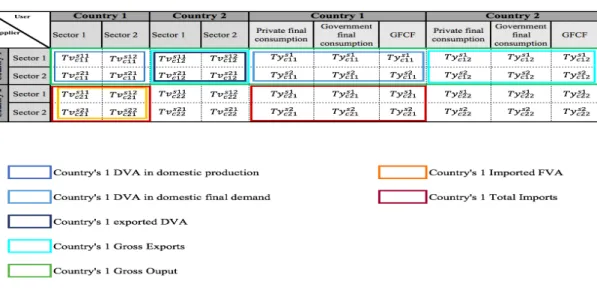
Figure II: Gross exports and Value Added Trade measures from the perspective of a 2 country, 2 sectors internationally linked IO database
Source: Author, based on Aslam et al. (2017) and Martinez-Galan (2018)
Figure II details the above-mentioned measures from an Internationally Linked IO table perspective in a two country, two sector world. 𝑇" represents trade in value added (or intermediaries) and 𝑇$ represents the trade that goes to final demand, 𝑐 represents the country and 𝑐&' represents the flows from country 1 to country 2, in the same way that s
represents a sector and 𝑠&' represents the flows from sector 1 to sector 2. That way,
taking the supplying Country 1 and Sector 1 as an example, 𝑇𝑣*&'+&' represents the
intermediaries from sector 1 and country 1 that are exported to Country 2 for production processes in sector 2. 𝑇𝑦*&'+& would represent the exports from Sector 1 in Country 1 that
15
3. Measuring Trade in Value Added for Countries in 2000 and 2014
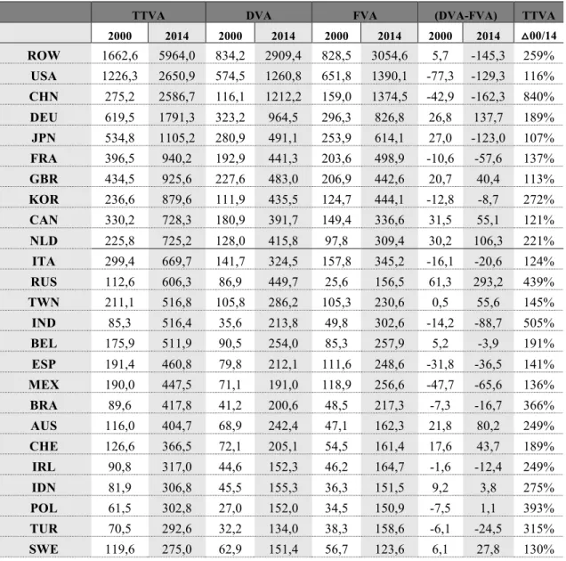
Table I details trade in value added indicators for 43 OECD countries, Emerging countries and the Rest of the World (RoW). Eligibility criteria for both country and time periods was WIOD’s 2016 release. It encompasses all countries available and data for the oldest (2000) and latest (2014) periods available. Table I includes absolute values in billion US dollars for TTVA, DVA and FVA and growth rate for TTVA (to get a sense of the world’s and country-specific growth of TVA). In addition, it includes gross measure of GVC positioning (DVA-FVA) based on Martinez-Galán and Fontoura (2018), that excludes the Gross Exports’ normalization but allows an overview of a country’s positioning as net exporter (DVA>FVA) or net importer (DVA<FVA) of value added.
Table I: Trade in value added measures for WIOD 43 countries and RoW
TTVA DVA FVA (DVA-FVA) TTVA
2000 2014 2000 2014 2000 2014 2000 2014 △00/14 ROW 1662,6 5964,0 834,2 2909,4 828,5 3054,6 5,7 -145,3 259% USA 1226,3 2650,9 574,5 1260,8 651,8 1390,1 -77,3 -129,3 116% CHN 275,2 2586,7 116,1 1212,2 159,0 1374,5 -42,9 -162,3 840% DEU 619,5 1791,3 323,2 964,5 296,3 826,8 26,8 137,7 189% JPN 534,8 1105,2 280,9 491,1 253,9 614,1 27,0 -123,0 107% FRA 396,5 940,2 192,9 441,3 203,6 498,9 -10,6 -57,6 137% GBR 434,5 925,6 227,6 483,0 206,9 442,6 20,7 40,4 113% KOR 236,6 879,6 111,9 435,5 124,7 444,1 -12,8 -8,7 272% CAN 330,2 728,3 180,9 391,7 149,4 336,6 31,5 55,1 121% NLD 225,8 725,2 128,0 415,8 97,8 309,4 30,2 106,3 221% ITA 299,4 669,7 141,7 324,5 157,8 345,2 -16,1 -20,6 124% RUS 112,6 606,3 86,9 449,7 25,6 156,5 61,3 293,2 439% TWN 211,1 516,8 105,8 286,2 105,3 230,6 0,5 55,6 145% IND 85,3 516,4 35,6 213,8 49,8 302,6 -14,2 -88,7 505% BEL 175,9 511,9 90,5 254,0 85,3 257,9 5,2 -3,9 191% ESP 191,4 460,8 79,8 212,1 111,6 248,6 -31,8 -36,5 141% MEX 190,0 447,5 71,1 191,0 118,9 256,6 -47,7 -65,6 136% BRA 89,6 417,8 41,2 200,6 48,5 217,3 -7,3 -16,7 366% AUS 116,0 404,7 68,9 242,4 47,1 162,3 21,8 80,2 249% CHE 126,6 366,5 72,1 205,1 54,5 161,4 17,6 43,7 189% IRL 90,8 317,0 44,6 152,3 46,2 164,7 -1,6 -12,4 249% IDN 81,9 306,8 45,5 155,3 36,3 151,5 9,2 3,8 275% POL 61,5 302,8 27,0 152,0 34,5 150,9 -7,5 1,1 393% TUR 70,5 292,6 32,2 134,0 38,3 158,6 -6,1 -24,5 315% SWE 119,6 275,0 62,9 151,4 56,7 123,6 6,1 27,8 130%
16
TTVA DVA FVA (DVA-FVA) TTVA
2000 2014 2000 2014 2000 2014 2000 2014 △00/14 AUT 85,8 264,5 45,4 137,5 40,4 127,0 5,1 10,4 208% NOR 82,3 237,6 60,2 158,8 22,1 78,8 38,2 79,9 189% CZE 36,5 204,6 18,0 99,7 18,6 104,9 -0,6 -5,3 460% DNK 70,9 198,8 34,4 94,7 36,5 104,1 -2,1 -9,4 181% LUX 36,2 170,6 18,6 81,7 17,7 88,8 0,9 -7,1 371% HUN 35,9 149,6 14,4 68,5 21,5 81,1 -7,1 -12,6 317% FIN 54,8 137,1 30,6 68,5 24,2 68,7 6,4 -0,2 150% ROU 15,9 104,3 7,6 52,2 8,3 52,0 -0,7 0,2 555% PRT 35,6 100,1 11,6 49,1 23,9 51,0 -12,3 -2,0 181% SVK 11,5 99,3 4,6 46,0 6,9 53,3 -2,2 -7,4 767% GRC 29,4 77,8 11,4 38,2 18,0 39,6 -6,7 -1,3 165% BGR 4,5 45,3 1,1 22,4 3,3 23,0 -2,2 -0,6 918% LTU 4,0 38,6 1,8 21,1 2,2 17,5 -0,4 3,6 858% SVN 9,2 36,3 3,9 19,2 5,3 17,1 -1,4 2,1 297% HRV 9,5 28,7 4,6 14,6 4,9 14,0 -0,3 0,6 201% EST 3,2 24,4 1,4 12,6 1,9 11,8 -0,5 0,8 652% LVA 3,2 19,2 1,5 10,1 1,7 9,1 -0,3 1,0 501% MLT 5,0 18,6 2,0 7,4 3,0 11,2 -1,0 -3,9 270% CYP 4,4 12,1 2,0 6,5 2,4 5,5 -0,4 1,0 173% AVERAGE 193,2 606,3 -- -- -- -- -- -- 214%
Source: Author’s calculations based on WIOD 2016 release. Countries ordered according to its 2014 TTVA, from highest to lowest. The last column indicates TTVA growth rate computed with the traditional growth rate formula. Average values for world’s TTVA and average change rate exhibited in last row.
The first aspect that stands out from Table I’s reading is that world’s average TTVA has more than tripled from 2000 to 2014. USA accounted for the highest TTVA for both periods considered and, at the same time, it was the country registering one of the lowest growth rates from 2000 to 2014, being considerable below world’s average. On the other hand, China was the country with the highest growth rate. In fact, China’s TTVA growth was impressive, from 275.2 billion US dollars to more than 2500 billion US dollars, totalizing a growth rate of almost 900%. Northern European countries such as Germany, France, UK and The Netherlands registered much more modest growth rates. Even though all these countries are part of the top ten of highest TTVA for 2014, they recorded modest growth rates, none of them exceeding the world’s average growth rate. On the contrary, other Central European countries registered much higher growth rates, which is the direct result of the integration in the world’s economy after the dismantling of the Soviet Union, with countries such as Poland and Czech Republic registering considerably high TTVA. They have more than quadrupled its value in 15
17
years with growth rates of 393% and 460%, respectively. Japan was the country that registered the lowest growth rate in the periods considered. However, other Asian economies such as India, Indonesia and South Korea all registered high growth rates, having all more than tripled its TTVA value in 15 years.
In sum, from Table I’s analysis one can conclude a general tendency: with the notable exception of China, the countries with the highest trade in value added are also the ones with the lowest growth rates. This is partially because they depart from 2000 with already high values of TTVA, whereas other countries such as Bulgaria, Slovakia, Slovenia and Romania depart from very low values, registering impressive growth rates. However, since it is not normalized by countries’ economic size, this measure should be used with caution.
If we subtract the DVA from FVA, we get a sense of a country’s position in the upstream or downstream side of GVC’s. Martinez-Galán and Fontoura (2018) used this indicator normalized by Gross Exports to analyse country positioning in GVC’s in 2011. Since this exercise only subtracts the absolute values of DVA and FVA we can only compare the signal with their results.
For both periods considered, USA and China are net importers of value added, as its FVA value exceeds that of DVA. Northern European countries such as Germany, the Netherlands and United Kingdom have kept their position in the upstream side of the production chain in the 15-year period considered. Japan, Belgium, Luxembourg and Finland are the only countries that moved from net exporters of value added to net importers, Japan’s case is much more evident because it accounts for a higher difference. Other Asian economies such as Taiwan and Indonesia are net exporters of value added whereas India and South Korea are in both periods downstream of GVCs. Central European countries that were previously under the soviet sphere stand out as countries moving from a net importer position to a net exporter position. This is the case for Poland, Lithuania, Latvia but also other European countries such as Slovenia, Croatia and Cyprus.
The Rest of World (RoW) is still the agglomerate of countries that accounts for the highest TTVA, having registered a significant growth rate (259%) in both periods.
18
However, one has to take in consideration the fact that the individual countries in the WIOD account for more than 80% of the world trade. There has been a big change in the RoW’s positioning in the GVCs going from a net exporter to a net importer of value added; this necessarily means that the individual countries in the WIOD are suppliers of value added to the RoW.
This analysis serves as a proxy to the world’s trade in value added network that will detail the bilateral flows of trade, allowing a further decomposition of value added flows between countries and thus providing an overview of IO relationships in the world’s economy.
4.World Trade Networks – Network analysis with traditional trade statistics
Many recognize a network as an intuitive way of representing world’s trade (Benedictis and Tajoli, 2011), (Kim and Shin, 2002) and (Serrano and Boguñá, 2003). According to Benedictis and Tajoli (2011), trade flows between countries can be naturally represented by a straight line (trade flows) connecting two points (countries). In fact, a network’s structure and/or visualisation consists of a set of points, called nodes or vertices with connections between them called edges or links. Furthermore, it’s possible to add complexity to the nodes or edges by weighting them. This property of networks plays an important role in the analysis of world trade and it is also intuitive as the extent of trade between a pair of countries (usually measured in monetary values of imports and/or exports) is treated as the link weight (Bhattarcharya et al., 2008), thus reflecting the different magnitudes of bilateral trade relationships. Kali and Reyes (2007) stress another feature of network visualisation: the possibility of adding a threshold that not only allows for a better visualisation but also allows conclusions about the backbone structure of world’s trade. In addition, a directed network fully captures the direction of flows. The nodes can be weighted to highlight the importance of specific countries in the WTW, in line to what Serrano and Boguñá (2003) call a perfect example of a real-world network that illustrates competitive relationships. Finally, network-based measures play an important role in explaining world trade.
Another potentiality of the network analysis method is that it permits a relational view of the world’s commerce rather than the focus on an individual country’s performance.
19
This contrasts with other traditional trade models such as gravity models, measures of comparative advantages and constant market share (Reyes et al., 2008). This method permits the visualisation of the complete structure of the world’s trade and the network-based measures are powerful tools for the examination of trade flows’ properties and patterns.
Several issues associated with world’s economic integration have also been analysed under the scope of network analysis. The issues range from the duality between Globalisation and Regionalisation (Kim and Shin, 2002), to world’s system division in a core-periphery system studied with international trade data (Snyder and Kick, 1979) or with aggregated trade data (Smith and White, 1992). More recently, Benedictis and Tajoli (2011) employed network-based measures to address some issues debated in recent trade literature: (i) the role of WTO in international trade, (ii) the existence of regional blocks in a globalized world and (iii) the dimensions of the extensive and intensive margins of trade.
Depending on the employed methods and the central point of discussion, network analysis has enabled authors along the years to reach different but important conclusions not only about the configuration of international trade, but also about wider issues concerning globalization.
There are two main fields of research deploying the network method in the analysis of world’s commerce, one emerged from political sciences and the other, initiated in the 2000s, emerged from the field of econophyisics. Essentially, the first one takes international trade as a starting point to analyse the world system theory based on the structure of the WTN and thus enables to analyse an individual country’s or a group of countries’ position in world’s trade and the second is more focused on the topological properties of the WTN.
In a seminal work, Snyder and Kick (1979) aimed to study the world’s system theory by presenting a blockmodel network analysis for four types of international interactions including trade flows circa 1965. Their analysis corroborated the theory by finding the presence of three different positions: Core (West Europe, North America, Australia and Japan), Semi periphery (some Latin American countries, Eastern Europe and some
20
Asian countries) and Periphery (most of the Asian continent and all African continent). In terms of interactions, they found that every block has more trade linkages with the core than with any other. Smith and White (1992) elaborated on Snyder and Kick (1979) analysis by focusing their analysis solely on world trade, included 3 moments of time (1965, 1970 and 1980) and used aggregated trade data in 15 types of commodities. The inclusion of three time moments allowed for a time analysis that reported stability over time and much more upward than downwards mobility. In addition, the disaggregation of trade data enabled different conclusions for different sectors. For instance, the authors found that the exports of high technology manufacturing goods flow primarily within the core and from the core to lower blocks. The inverse is true for agricultural products where international trade is more likely to happen from the periphery to the core. The more recent analysis from Mahutga (2006) allows for an update in Smith and White’s (1992) results since it departs from the same 15 commodity types and adds the years 1990 and 2000 to the previous analysis. The main conclusion was that the hierarchical nature of the world system remained stable from 1965 to 2000 both in terms of core/periphery patterns of interaction and production processes and that the most noticeable change was the rise of labor intensive manufacturing in non-core zones such as Eastern European countries and the so called Asian tigers.
Reyes et al. (2008) disaggregated international trade data in four types: raw materials, intermediary goods, final goods and capital goods. Their network analysis aimed to enrich the exploratory literature about the rise of the BRIICS performance in the world system. For 1995, 2000 and 2005, they found an ever-increasing performance for the BRIICS in all the indicators percentile rankings they computed. The centrality index suggested that the BRIICS (with the exception of Indonesia) are highly integrated in the WTN or that they are increasing their level of integration with some differences between countries and product types. The analysis of the node strength, node degree and clustering suggest that these results are explained by multiple factors from the establishing of new trade partners to the involvement in trade clubs following the diminishing the role of the rich club and the intensification of existing trade relationships.
21
The articles with a more exploratory character of the WTN properties have also reached important conclusions upon the best way of representing world trade in a network. The focus here shifts from the hierarchical position of countries within the WTN to the correlation of network-based measures to explore the properties of world trade.
To this end, Garlaschelli and Loffredo (2005) break from previous studies focusing on a single snapshot of the WTW and address it as a directed and evolving network during 1950-1996. By correlating three topological properties of the WTW, they concluded that there is a negative correlation between of average nearest neighbor and degree distribution, which means that countries with many trade partners are on average connected to countries with few partners. In addition, they found a decreasing trend between clustering coefficient and degree distribution meaning that partners of well-connected countries are less interwell-connected than the partners of poorly well-connected countries (dissortative network). Fagiolo et al. (2008) challenged the topological properties of the WTW found in previous studies including that of Garlaschelli and Loffredo (2005). They argue that the binary approach to the world trade network is not accurate as it treats every trade link as homogeneous regardless of their actual value and use a weighted approach instead. They concluded that for weighted networks the dissortativeness is not statistically significant. In weighted networks, well-connected countries are associated with higher clustering coefficients, which confirms the existence of trade clubs. Serrano et al. (2007) built and analyzed the world network of trading imbalances. In their network, the links represented the difference between exports and imports and were weighted by the magnitude of that difference. By applying a local heterogeneity analysis, the authors obtained the backbone of the WTN for 1960 and 2000, which corresponds to the links that carry the biggest proportion of a country’s inflow or outflow. Furthermore, the authors have taken a first step into the study of GVCs using traditional trade data, by considering that producer and consumer countries do not absorb completely the incoming or outcoming flux. By conducting a dollar experiment for the two major source countries and two major sink countries, Serrano et al. (2007) clearly distinguished between the percentage of net dollars that goes into bilateral trade and the allocation of these net dollars in the world system. For instance, they found that for each net dollar that USA injects into the system only 9.3% is retained in China although the direct connection imbalance between the two countries is 16.7%.
22 5. Networks of trade in value added – Network analysis with input-output trade statistics
In the same way than the research in GVCs, the use of the network analysis method for input-output trade data is recent and will certainly be subject to further analysis and developments. Nevertheless, the authors employing the network analysis to date reinforce its potentialities to understand trade in value added. Some discuss that the complexity of the measures in the network theory and the ability to build models that incorporate these features are powerful tools to understand GVCs (Amador and Cabral 2015). Others argue that network analysis enables the analysis of the heterogeneity of different actors and trade links in GVCs (Santoni and Taglioni, 2015) and that network-based measures can be correlated to the presence of external factors such as the presence of multinational groups (Altomonte et al., 2015). Once again, it is an intuitive mode of representing trade in value added as IO tables are themselves weighted and directed networks.
Even at its early stages, the literature applying network analysis to GVCs revolves around two major outbreaks: (i) the analysis of countries and countries-sector positioning and (ii) propagation of economic shocks along the production network. The first stream applies network-based measures to derive conclusions about either the countries or country-sector positioning in the production networks and the second stream complements the study of these measures by correlating them with external factors that enable conclusions about what countries or sectors are most vulnerable to the persistence and/or propagation of economic shocks.
Amador and Cabral (2015) made use of basic network visualization tools to describe the characteristics of GVCs, using WIOD data for 40 countries in 1995 and 2011 that represented bilateral flows of FVA. Their conclusions focused mainly in individual countries’ centrality, finding that bigger countries tend to have higher nodes and appear in the center of the network as suppliers of value added. In terms of evolution they found that, in 1995 the countries in the core were mainly Western European and the USA, whereas Asian countries were located in the periphery. By 2011 some of these countries (UK and France) partially lost their positioning but USA and Germany are
23
still at the core and China joined the center as the most important supplier of value added. In addition, the authors built the world’s networks for manufacturing goods and services to conclude that the density of the manufacturing network is much higher than that of the services network, meaning that nations are more interconnected in the trade of manufacturing goods.
Focusing in country-sectors rather than on solely individual countries, Santoni and Taglioni (2015) computed the network of intra-sectoral trade for the automotive sector (buyers and suppliers network) and the network for trade in value added for country-sectors in 2009. They conclude that the increasing centrality of emerging countries is most prominent in the demand side than in the supply side in technology intensive GVCs and that US industries are still at the core of the network of global trade alongside German business services, China’s retail and Russian mining. Cerina et al. (2015) configure the world trade system as a network where the nodes are the different industries from different countries for 1995 and 2011 including self-loops that represent intra-industry national trade. They find that the trade network is denser inside the same economy than in-between economies; this means that great part of the economic transactions still occurs within national borders and contains many self-loops (high number of industries self-feeding themselves). At the regional level, they employ a community detection analysis that compares their network with a null model graph that carries the assumption that a random graph is not expected to have a community structure. They conclude that global production is still operated nationally or, at best, regionally, given that the detected communities are individual economies or well-defined geographical regions (e.g. NAFTA countries). Criscuolo and Timmis (2018) applied the “Bonacich-Katz” eigenvector centrality metric to OECD ICIO data and calculated metrics based on forward and backward linkages. They illustrate that there have been profound changes in the structure of GVCs over the period 1995-2011. Whilst some activities remain clustered around the same key hubs as in the start of the period, for others there have been dramatic relocation of the economic activity (e.g. manufacturing of computer and electronic sector). At the country-level, they report the evolution around three main world regions: Factory Europe, Factory Asia and Factory America. The evolution is significant, with the consolidation of Germany and USA as central hubs in their respective regions and the diminishing role of Japan as a key hub in Asia where China now plays a central role.
24
Carvalho (2014) argues that the structure of the production networks is crucial in determining whether and how microeconomic shocks (affecting only a particular firm or technology along the chain) propagate through the economy as these production networks expose critical nodes in these chains. This is particularly evident when a small
number of central hubs supply inputs to many different firms or sectors. Still, in the context of the use of network analysis to assess propagation of economic shocks along production networks, Blochl et al. (2011) computed two network measures of centrality: random walk and counting betweeness centrality. The first one is important to reveal the vertices instantaneously affected by a shock and the second one to reveal where a shock carries on longer. In addition, Blochl et al. (2011) computed the hierarchical clusterings of the nodes’ rankings in the network to find that countries with similar levels of development tend to group together. Taking on the economically non-meaningful character of previous studies, Contreras and Fagiolo’s (2014) proposed the application of a diffusion model that took into consideration the origin of the shock, its impact on IO linkages and the possibility that after the shock hits a certain sector, the production levels adjust.
Figure III sums the main streams of literature employing network analysis to trade by segmenting it in traditional trade statistics and in TiVA. One can argue that exist some similarities in the conclusions of those studies. For instance, the network-based measures are essentially the same. Moreover, some authors using the network analysis
Figure III: Main branches of literature for network analysis in trade and in TiVA Source: Author
25
for trade have taken small steps to the study of GVCs by decomposing traditional trade statistics into several commodity types, having reached different conclusions for different sectors.
However, differences are more striking given the fact that one is a trade network and the other is a production network. This has repercussions in the type of issues studied by each. From the perspective of networks utilizing traditional trade statistics, the focus is either on the inequality provoked by the asymmetries in world trade whereas in the networks of trade in value added several authors have studied the propagation of economic shocks by assuming the interdependencies between countries and sectors in the network. Another important contrast is that the literature in traditional trade statistics emphasizes much more the rise of emerging economies. Studies of networks of trade in value added also acknowledge it but alert that their centrality varies in parallel to the sector in consideration.
6. The world users and suppliers network (2000 and 2014)
The present chapter makes use of the indicators computed in section 4 and combines them with computed bilateral trade flows to visualize the world’s users and suppliers network.
There are two fundamental identities to define before building a network: the nodes and the linkages between them. In this case, the nodes are the 43 countries available in the WIOD and the links or edges are the bilateral trade in value added flows amongst them for 2000 and 2014. Even though the WIOD includes the RoW, it is excluded from the network visualisation and from further network-based calculations because as an aggregate of economies it would profoundly influentiate the network nodes and edges weights since it embodies a disproportionate number of economies to whom TiVA data is not specified.
In this network, the nodes are weighted according to the countries’ TTVA (defined in section 3), with higher diameters representing higher values of TTVA. The edges are weighted according to the size of the bilateral trade flows between countries with higher thickness accounting for higher trade in value added flows. Futhermore, the links are colored according to it’s value with dark grey indicating the 10% highest flows and even darker grey representing the Top 10 of highest bilateral value added flows. With
26
the nodes weighted by TTVA and the edges representing the world’s suppliers and users of value added it’s possible to break out a country TTVA, getting a sense of the worlds suppliers and users and more specifically how DVA and FVA split along the world’s economy.
Another important aspect of this network is the fact that it is directed, allowing the visualisation of the trajectory of bilateral value added flows. In this case the arrow points to the destination country (user). Two important network concepts are associated with this visualisation: the indegree and outdegree; indegree refers to the number of incoming edges (user country) and the outdegree refers to the number of outgoing edges (supplier country).
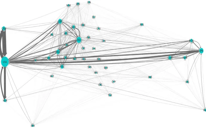
Figures IV and V represent the world’s suppliers and users network for 2000 and 2014 respectively. To facilate visualisation without compromising the most relevant flows and not excluding any of the 43 countries, a threshold was defined. Only flows accounting for 1% of user or supplier countries’ TTVA appear. Further analysis and calculations of network-based measures will be conducted using this threshold. Countries in the network are displayed according to their location.
Figure IV: The world’s users and suppliers network, 2000
Source: Author, the graph is built with the use of cytoscape an open source software, originally designed for biological research but now a general platform for complex network analysis and visualization.
27 7. Network visualisation and network-based measures
Network-based measures are crucial to a fully-comprehensive analysis of a network, allowing the identification and analysis of connections, connection’ patterns and centrality. In addition, as previously discussed, one can employ statistical techniques to visualize how those measures interact with each other and re-inforce the economical meaning of the conclusions. At the same time, there is a lot one can conclude from simple network visualisation, depending whether the nodes and edges are weighted or not. This is the case for changes through time, intensity of bilateral trade flows and global, regional and local densities. This section presents the main conclusions of this work. It starts by discussing the results of network visualisation and of the application of some descriptive statistics and ends with the comparative analysis of two network-based measures.
From the observation of Figure IV one can see that in 2000 the bilateral flow with the highest value was by far the one from Canada to USA with the opposite flow in the
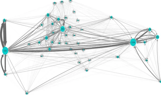
Figure V: The world’s users and suppliers network, 2014
Source: Author, the graph is built with the use of cytoscape an open source software, originally designed for biological research but now a general platform for complex network analysis and visualization.
28
second position. Factory America is clearly dominated by the USA, which is not only the country with the biggest node, but also accounts for the thickest to and from intra and inter regional flows; most of the flows to and from USA are also colored with dark grey, which means that in 2000 most of the flows coming into and out of this country belonged either to the 10% highest flows or to the Top 10 highest flows. Other noticeable high flows are the ones from USA to Japan. Japan was in 2000 the country with the highest TTVA in Factory Asia, with intra regional flows being oriented towards and from this country. However, Japan’s centrality within Factory Asia was not as visually evident as the one from USA in Factory America, other asian countries such as China, South Korea and Taiwan already exhibited strong positions within the region. Nevertheless, in 2000 the thickest flows within this region were the bilateral flows from South Korea to Japan and from Japan to South Korea. As for Factory Europe, Germany is the country with the highest TTVA, with other western-european being relevant players as well. In Europe, the highest intra-regional flows were those inbetween western-european countries. Inter-regional flows to USA exhibit dark grey color, which means that some of them (e.g. UK to USA) are among the Top 10 highest flows.
In 2014, the flow from Canada to USA remains the highest flow of TiVA and the second position still belongs to the opposite flow. USA remains the country with the highest TTVA in Factory America with the highest intra and inter-regional flows. Factory Asia accounted for the biggest changes in the 15 years’ period; not only the central position has shifted from Japan to China, but also the density of intra and inter regional trade has augmented substantially, containing darker and thicker links. In Factory Europe, Germany remains the country that accounts for the highest TTVA, but one clearly sees that trade intensity has also increased within the region with more participation from Eastern European countries, with flows mainly to and from Germany. Conversely, the flows between this region and USA seem to have comparatively lost relevance within the world flows. They have lost their dark grey tonality, which means they are no longer amongst the Top 10 highest flows. Another particularity is that outward flow from China to USA is higher than the opposite flow, meaning that China is a net supplier of value added to the USA. Although this contradicts the theory that the USA does not have a trade in value added imbalance with China; the analysis lacks, however, further sector decomposition.
29
Table II shows that flows making 1% of the supplier or users TTVA have slightly grown from 2000 to 2014; this is also true for the total TTVA which has more than trippled its value. Distribution wise, Table II also shows that both mean and median values are low and much more closer to the lowest bilateral flow which means that the distribution of bilateral TVA flows is left-skewed, which we can comprove by a larger mean value than the median value.
The left bias of the distribution is further corroborated by the trade flows intensities’ displayed in Table II, where we can see a small number of flows accounting for the most part of the TTVA flows. However, the results are slightly different in 2000 and in 2014. In 2000 only 17 countries made up 50% of the world’s TTVA and in 2014, more than half (23) of the countries in analysis accounted for half of the world TTVA flows. Over time, we see an increase of countries’ participation in production networks. At the same time, there was still a small number of countries that do not have a substantial participation in the production networks, as only 34 and 35 of the 43 countries were included in 90% of the world’s TTVA in 2000 and 2014, respectively.
From network visualisation one can see that the number of flows have increased over time, meaning that the network density has increased. Density is an important network concept, it is the ratio between the total number of connections and the total possible ranging from 0 to 1. In this case, if it wasn’t for the threshold this network would have a total density of 1 as in the IO tables all countries have flows with each other, as the focus here is only on the most relevant trade flows the density goes from 0,39 in 2000 to 0,40 in 2014. Density interacts directly with another fundamental network identity, which is node degree.
Table II: Descriptive statistics and flow intensities
2000 2014
Total No of Countries 43 43
Total No of flows 713 730
Total value of TTVA (Billion US dollars) 2408,7 6790,7
Lowest bilateral flow (Billion US dollars) 2,1 7,0
Highest bilateral trade flow (Billion US dollars) 874,1 1885,2
Average TTVA (Billion US dollars) 3,4 9,3
Median TTVA (Billion US dollars) 1,0 3,4
No of countries making up 50% of TTVA 17 23
No of flows making up 50% of TTVA 45 57
30
Source: Author’s calculations based on WIOD IO data for 2000 and 2014
Node degree in directed networks divides into outdegree and indegree. Weighted networks permit the analysis of node strenght, which for directed networks also divides into indegree strenght and outdegree strenght. The last three network concepts are also three fundamental indentities of this weighted and directed network: (i) node strenght is equal to a countries’ TTVA, (ii) indegree strenght is equal to a countries’ FVA and (iii) outdegree strenght is equal to a countries DVA. Having a look at the correlation of both measures, one can conclude about the existence of a positive or negative relationship between the total number of TiVA partners and the TTVA value. The world users and suppliers networks exhibits a strong correlation (≈0.75) for both periods, which means that the countries with a higher number of partners have higher TTVA values. This correlation has slightly decresased from 2000 (0.76) to 2014 (0.75), which can be explained by a big increase in TTVA values with a constant number of world countries in analysis. The correlation of both indegree and outdegree strenght tell us that there is an almost perfect relationship (r>0.95) between countries in the upstream or downstream margins of GVCs, that is, great suppliers tend also to be great users of value added. Annex 1 displays the calculations of node degree and node strenght for all countries in 2000 and 2014.
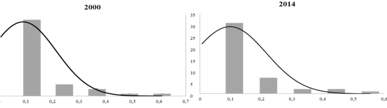
Looking at the distribution of node degree in Figure VI one can confirm that it is highly left-skewed with most of the countries in 2000 and 2014, having between 15 and 45 (out of 85) partners for both inward and outward flows of value added, there’s no bimodality in the distribution.
The distribution is even more left-skewed when one takes into consideration the flows’ values, as displayed in Figure VII. Most of the countries in the network hold weak TiVA relationships, while few of them account for the highest values in the distribution. The middle classes are empty or account for low values in both periods, which reinforces the uneven distribution of the production chain. Nevertheless, in 2014, there are more countries in the higher classes than in 2000. Table III displays the countries
No of flows making up 90% of TTVA 260 316
% of TTVA belonging to the top 10% flows 61,7% 56,3%
31
that account for the highest and lowest shares of indegree and outdegree strength. As the abovementioned correlation between both indicators would predict, the top countries for indegree strength are almost the same as the top five countries for outdegree strength. This is the case for both periods considered and for the bottom five countries.
Figure VI: Total node degree distribution 2000 and 2014
Source: Author calculations based on WIOD IO data for 2000 and 2014
Figure VII: Total node strengh distribution 2000 and 2014
32
Table III: Top 5 and Bottom 5 countries in Indegree and Outdegree Strenght Percent Rank Analysis
Source: Author calculations based on WIOD IO data for 2000 and 2014. Full percent rank analysis available in Annex 2.
An important conclusion from the Percent Rank analysis available in Annex 2 is that smaller countries tend to have lower positions. Table III confirms this, with the exception of Bulgaria that has noticeably moved out of the bottom five from 2000 to 2014, the same four small European countries share the bottom positions in both periods. However, the top five positions are shared between big and medium countries. USA is the country with the highest inward and outwards flows of value added for both period considered. Few has changed in 15 years with the noticeable and well documented rise of China as a supplier and user of value added in detriment of Japan who has lost its position in the top 5 countries with the highest DVA and FVA. In addition, China has entered directly to the third position surpassing western European countries such as the UK and France. Another relevant supplier of value added is the Netherlands, which in 2014 has the fourth position in terms of indegree strength; in figure 5 is possible to envisage that the arrow from this country to Germany is within the Top 10 highest flows of TiVA.
Node strength and Node Degree are also considered centrality measures, but these capture only direct links and neglect indirect linkages, therefore, to fully understand a country’s positioning in the users and suppliers network, Eigenvector Centrality is a good complement to those node-related measures.
Eigenvector as calculated by the Tang’s et al. (2015) formula - based on Bonacich’s
Indegree (FVA) Strenght Outdegree (DVA) Strenght
2000 2014 2000 2014
Top
5
USA USA USA USA
DEU DEU DEU DEU
FRA CHN JPN CHN GBR FRA GBR NLD JPN GBR FRA GBR Bottom 5 BGR LTU CYP HRV CYP MLT LTU MLT
LTU EST EST EST
LVA LVA LVA CYP
33
(1987) work - is a node centrality index. The rationale behind Eigenvector Centrality is that connections to high-scoring nodes contribute to the score of the node in question. Consequently, this measure contemplates indirect linkages. This is the main difference from other measures of centrality such as closeness centrality and betweeness centrality, which disregard neighbours’ score. Criscuolo and Timmis (2018) use a variant of this measure in their work, stating that the existence of multiple linkages should be took into consideration, as it is a real world network feature where service linkages are needed at several stages of production processes.
The distribution for the Eigenvector Centrality is, once again, left-skewed, meaning that most of the countries do not hold meaningful supply-use relationships (Figure VIII). The tendency has been constant in both periods considered with a slight overall increase in the middle classes in 2014.
Figure VIII: Eigenvector centrality distribution 2000 and 2014
Source: Author calculations based on WIOD IO data for 2000 and 2014. Full percent rank analysis available in Annex 2.
Table IV displays the correlation between Node Centrality and Eigenvector Centrality. They are all positive, which means that more and more intense direct supply-use relationships contribute to a more central position within the network. An interesting aspect is that the correlation with Node Strength is much more statistically significant than the correlation with Node Degree, emphasizing the character of this measure that neglects the number of partners in favour of their importance within the network. Countries such as Canada and Mexico have a low number of partners but they are strongly connected to USA, which has a high centrality, therefore they also account for a high Eigenvector Centrality. The opposite occurs in countries such as Belgium and
34
Italy who have a relatively high number of trade partners who are only moderately central within the network. The percent rank analysis available in Table V seems to display the same Top and Bottom countries as the Indegree and Outdegree Strength percent rank analysis.
Table IV: Correlation coefficient of centrality measures
2000 2014
EC - NS 0,94 0,92
EC - ND 0,58 0,59
Source: Author calculations based on WIOD IO data for 2000 and 2014. Formula for eigenvector centrality follows Tang et al. (2015).
Table V: Eigenvector centrality percent rank analysis
Percent Rank 2000 2014 To p 5 USA USA CAN CAN DEU DEU JPN CHN GBR NLD Bo tt om 5 HRV HRV LVA MLT BGR EST LTU LVA EST CYP
Source: Author calculations based on WIOD IO data for 2000 and 2014. Formula for eigenvector centrality follows Tang et al. (2015).
One noticeable difference between Node Strength percent rank analysis and that of the Eigenvector Centrality is that Canada is in the second position, due to its connection to the USA. China has entered the fourth position in 2014, meaning that the country is well established in the supply-use networks; however, when comparing with Node Strength’s third position one can conclude that China’s relevance is bigger when we take into consideration the intensities of the flows with its direct partners. Another significant change is the entrance of the Netherlands to the second position: from Node Strength