Finance from the NOVA – School of Business and Economics.
DISSECTING INFLATION IN BRAZIL
André Sereto da Costa Benedy, nº 4057
A Project carried out on the Master in Finance Program, under the supervision of: Professor Martijn Boons
2
DISSECTING INFLATION IN BRAZIL
Abstract
This paper investigates the short and long-term dynamics between inflation and four variables – money supply, real broad effective exchange rate, real interest rate and unemployment – in Brazil. The data sample ranges from 2002 until 2018. I make use of a vector error correction model and find that every explanatory variable is statistically significant in explaining inflation over the short and long-run. Except for the real interest rate, the individual relationships are in accordance with the findings of relevant literature. I also compare the model’s out-of-sample performance with the top short-run Brazilian CPI forecaster, as selected by the Brazilian Central Bank.
Keywords
3 I. Introduction
Understanding the dynamics of inflation is a matter of utmost importance for central banks, in the sense that only by doing so they can pursue effective policies in a recurrent fashion. The tools possessed by these entities allow them to influence several aspects of an economy, be it the amount of money that is in circulation at a given time, the value of a country’s exchange rate, the basic interest rate of the economy – which effectively determines the level at which the majority of interest rates will settle at –, among others. In other words, central banks are able to influence aggregate demand and supply so as to achieve a set of goals, chief among which is guaranteeing price stability. Pursuing a stable and low rate of inflation is imperative for an economy, since it offers a lower degree of uncertainty, which is vital for business development and investment, while simultaneously allowing for the channeling of resources to more productive and wealth-generating uses, instead of less productive and wealth-protecting solutions in periods of high and unstable inflation (e.g. portfolio management).
This paper sets out to determine the short and long-run relationships that exist between inflation and four variables – money supply, real broad effective exchange rate, real interest rate and unemployment – in Brazil. In doing so, it shines a light on how Brazilian authorities and investors can foresee inflation fluctuations before these happen, and thus either make policy adjustments in a timely manner or manage wealth allocation to reduce the risk of financial losses. This study adds value to currently available literature by attempting to dissect Brazilian inflation in an updated dataset, through the establishment of a co-integrated long-run relationship between inflation and the aforementioned independent variables, as well as through the use of a vector error correction model to portray the short-run dynamics of this interaction. The remainder of this paper contains four sections. Section two offers a review of relevant literature. Section three describes both the data and the methodology used in this study.
4 Section four presents the main empirical findings and offers a discussion. The fifth and final section concludes the study and derives some policy implications from the main findings of the previous section.
II. Literature Review
A significant amount of research has been made in an attempt to uncover what are the root causes of inflation, with some of most commonly mentioned including an expansionary monetary policy, falling interest rates and unemployment, and a rising output gap. Besides these, other studies find significant relationships between inflation and variables such as international oil price, foreign exchange rate, wage growth, labor productivity and government expenditure.
Friedman (1956) found a significant and positive relationship between an expanding money supply and inflation, which was later corroborated by the findings of Lucas (1980) and Dwyer and Hafer (1988). Unemployment was found to have a significant and negative impact on inflation by Phillips (1958), who introduced the Phillips Curve. Devereux (1989) documents that instability of real output measures exert a positive impact over inflation. According to Hooker (2002), a shock in oil prices was found to cause inflation in a sample ranging from 1962 to 1980, but the same did not remain true for the following two decades. Augustine et al. (2004) established a significant and positive interaction between exchange rate volatility and inflation. The findings of Tillmann (2008) point towards a positive relation between interest rates and inflation, due to the former generating an increase in marginal costs that is then released onto the economy via the supply side. Lim and Sek (2014) find government expenditure is a significant variable in explaining long-run trajectory of inflation in high inflation countries.
5 A point worth mentioning is that these dynamics are not confined to developed economies. For Pakistan, Khan and Gill (2010) uncovered a positive relationship between inflation and an expanding money supply, exchange rate and budget deficit. For Tanzania, Laryea and Sumaila (2001) discovered evidence of a positive influence on inflation coming from an expanding money supply and the exchange rate, whereas the country’s growth in terms of gross domestic product appears to drive down inflation. Lim and Papi (1997) found money supply and wage growth had a positive impact on Turkey’s inflation, while exchange rate presents the opposite dynamic. Odusanya and Atanda (2010) found evidence of Nigerian inflation having a positive relationship with variables such as the growth rate of the country’s gross domestic product, money supply and interest rate. Pahlavani and Rahimi (2009) determined that Iran’s inflation is positively linked to money supply growth, gross domestic product and exchange rate.
III. Data and Methodology
With the goal of understanding the dynamics between inflation and selected explanatory variables in Brazil, quarterly data ranging from the first quarter of 2002 until the third quarter of 2018 was collected for inflation (CPI), money supply (M2), real broad effective exchange rate1 (RBEER), real interest rate (RIR) and unemployment (UNEMP). Sources include Instituto
Brasileiro de Geografia e Estatística (IBGE), Banco Central do Brasil (BCB) and Federal Reserve Economic Data (FRED). The starting point of the collective time series was determined
by the first available entry for quarterly unemployment data (i.e. first quarter of 2002). To summarize:
1 The real broad effective exchange rate is measured as an index, with 2010 = 100, and it increases in value when
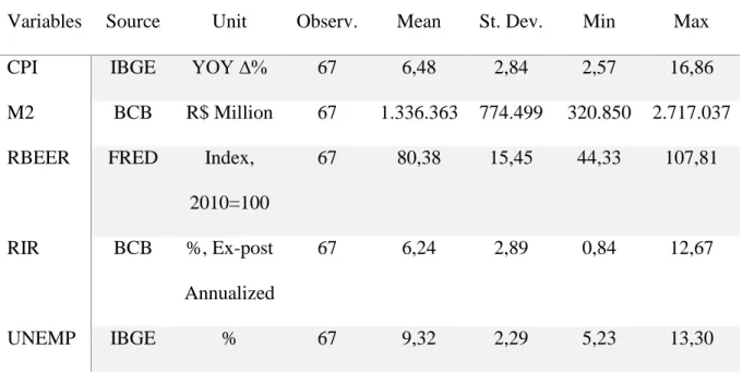
6 Table 1: Descriptive Statistics
Variables Source Unit Observ. Mean St. Dev. Min Max
CPI IBGE YOY ∆% 67 6,48 2,84 2,57 16,86
M2 BCB R$ Million 67 1.336.363 774.499 320.850 2.717.037
RBEER FRED Index,
2010=100 67 80,38 15,45 44,33 107,81 RIR BCB %, Ex-post Annualized 67 6,24 2,89 0,84 12,67 UNEMP IBGE % 67 9,32 2,29 5,23 13,30
7 In order to make the interpretation of results a matter of elasticity, I convert both M2 and RBEER into logarithmic form, which allows every coefficient obtained to be interpreted as the percentage impact that a one percent change in the value of a certain explanatory variable has on the dependent variable. As such, the base model can be specified as:
1) CPI = f ( logM2, logRBEER, RIR, UNEMP )
2) CPIt= α + β1logM2t+ β2logRBEERt+ β3RIRt+ β4UNEMPt+ µt
Where, apart from those mentioned previously, α refers to the constant term, βi to the coefficient
of independent variable i and µ to the error term.
Acknowledging that macroeconomic variables are likely to be trended, thus potentially verifying spurious relationships with each other, it is of utmost importance to understand whether the variables included in this study possess a unit root (i.e. are non-stationary) or not (i.e. are stationary). To that end, I begin by investigating whether each chosen variable follows a stationary process by applying the Augmented Dickey-Fuller (ADF) test. So as to increase the robustness of the results, I conduct every stationarity test i) including only a constant term and ii) including both a constant term and a linear time trend. I start by checking if the variables are stationary at level and, if non-stationarity is the case, I apply the aforementioned testing procedure at first difference.
Afterwards, the optimal lag length is determined based on several lag-order selection criteria, namely Final Prediction Error (FPE), Akaike Information Criterion (AIC),
Hannan-8 Quinn Information Criterion (HQIC) and Schwarz Information Criterion (SBIC). The goal of using these information criteria is to strike the best balance between goodness of fit and the parsimonious specification of the model, or, in other words, to ensure the model achieves a high explanatory power using as little explanatory variables as possible. Given the fact that this study resorts to quarterly data, the lag-order selection process uses as reference a maximum possible lag of 8 periods (i.e. 2 years), thus moving the first non-lagged observation in the time series from the first quarter of 2002 to the first quarter of 2004.
Then, the Johansen Co-Integration test is carried out to investigate the existence of a long-run equilibrium relationship (i.e. co-integration) between the variables by making use of two likelihood estimators for the co-integration rank – the trace statistic and the maximum eigenvalue statistic. Co-integration is said to exist between non-stationary variables if a linear combination of these is stationary. As such, the test is appropriate for a time-series that is non-stationary at level, but non-stationary at first difference (i.e. integrated processes of order 1, or I(1) processes), and is preferred over other methods for its ability to estimate multiple co-integration relationships simultaneously.
A vector error correction model (VECM) is estimated next, with the estimation period ending in the last quarter of 2014. This model represents a restricted version of a vector autoregressive (VAR) model to which error correcting features are added, and is employed when a multivariate time series is known to be both non-stationary and co-integrated so that, apart from the long-run equilibrium relationship revealed by the co-integration test, one can analyze the short-run dynamics between variables. In the case of this particular study, the vector error correction model can be specified as:
3) ∆CPIt= γ + λ1∑kj=1∆CPIt−j+ λ2∑kj=1∆logM2t−j+ λ3∑kj=1∆logRBEERt−j+ λ4∑kj=1∆RIRt−j+ λ5∑kj=1∆UNEMPt−j+ ψECMt−1+ εt
9 Where ∆ refers to the difference operator (used due to stationarity only being verified at first difference), γ to the constant term, λi to the coefficient of independent variable i, k to the
selected lag length, ψ to the error correction term (i.e. the speed of adjustment term) and ε to the error term. If the error correction term (ψ) is both negative and statistically significant, any short-term fluctuations between dependent and independent variables will eventually converge back into a stable long-run equilibrium relationship. In other words, a short-term shock to this interaction will reverse back to its long-run equilibrium at the speed of - ψ % per period.
Subsequently, diagnostic tests are performed with the goal of investigating whether the residuals generated by the model are autocorrelated and normally distributed.
To conclude, I use the specified vector error correction model to forecast Brazilian CPI values out-of-sample from the first quarter of 2015 until the third quarter of 2018. The resulting residuals are then compared against those obtained by the top short-run Brazilian CPI forecaster, as selected by the Brazilian Central Bank (BCB), through the relative root mean squared error (RMSE) measure.
IV. Results and Discussion
Unit Root Test
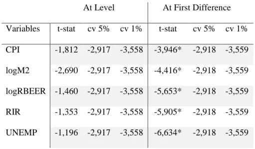
The null hypothesis of an Augmented Dickey-Fuller test is that the variable being examined is non-stationary (i.e. has a unit root), and it is rejected when the value of the Augmented Dickey-Fuller t-statistic is lower than the corresponding critical value at the preferred level of statistical significance.
By observing table 2, we can verify that the null hypothesis cannot be rejected at either the 1% or the 5% level for the variables at level, either when we include only a constant term
10 or when we include both a constant and a trend term. Regarding the variables at first difference, I find that the null hypothesis is rejected at the 1% level for almost every variable in both versions of the test, with CPI being the only exception since it rejects the null hypothesis only at the 5% level when both a constant and a trend term are considered. As such, we can conclude that every variable included in this study is integrated of order 1, I(1), which is to say they only achieve stationarity at first difference.
Table 2: Augmented Dickey-Fuller Test Results
In the following table, * and ** indicate statistical significance at the 1% and 5% levels, respectively.
i) With constant term
At Level At First Difference Variables t-stat cv 5% cv 1% t-stat cv 5% cv 1% CPI -1,812 -2,917 -3,558 -3,946* -2,918 -3,559 logM2 -2,690 -2,917 -3,558 -4,416* -2,918 -3,559 logRBEER -1,460 -2,917 -3,558 -5,653* -2,918 -3,559 RIR -1,353 -2,917 -3,558 -5,905* -2,918 -3,559 UNEMP -1,196 -2,917 -3,558 -6,634* -2,918 -3,559
ii) With both constant and trend terms At Level At First Difference Variables t-stat cv 5% cv 1% t-stat cv 5% cv 1% CPI -1,946 -3,484 -4,115 -3,907** -3,485 -4,117 logM2 0,224 -3,484 -4,115 -4,732* -3,485 -4,117 logRBEER -1,246 -3,484 -4,115 -5,661* -3,485 -4,117
11 RIR -2,004 -3,484 -4,115 -5,854* -3,485 -4,117
UNEMP -0,849 -3,484 -4,115 -6,869* -3,485 -4,117
Lag-order Selection
The optimal lag length is determined by minimizing the values of the various lag-order information criteria employed in the test.
As can be seen in table 3, there is no absolute unison between the various decisions, with the information criteria FPE, AIC and HQIC selecting 5 lags while the SBIC criterion only advises the selection of 2 lags. This being the case, I settle upon the choice of the majority – 5 lags – and use it to carry out the upcoming Johansen Co-Integration test and the estimation of a vector error correction model.
Table 3: Lag Length Selection Results
In the following table, * refers to the optimal lag length that is chosen by the corresponding information criterion.
Lag FPE AIC HQIC SBIC
0 2,1e-15 -19,6200 -19,5448 -19,4172 1 8,3e-20 -29,7494 -29,2983 -28,5329 2 1,1e-20 -31,7986 -30,9716 -29,5684* 3 9,0e-21 -32,1389 -30,9358 -28,8949 4 6,4e-21 -32,7263 -31,1474 -28,4686 5 4,3e-21* -33,5803* -31,6254* -28,3088
12 Johansen Co-Integration Test
The first null hypothesis of a Johansen Co-Integration test states that there is no co-integration between the variables selected and it cannot be rejected if the statistic being used (either the trace statistic or the maximum eigenvalue statistic) has a value lower than the corresponding critical value at the preferred level of statistical significance. If the opposite happens and the null hypothesis is rejected, we proceed into the second null hypothesis – there is one co-integrated equation among the variables. The same criterion for rejection is applied and we follow this procedure until we reach the first iteration where the null hypothesis cannot be rejected.
Table 4 reveals that both the trace statistic and the maximum eigenvalue statistic point towards the existence of co-integration, with the former indicating the presence of four c-integrated equations while the latter signals the presence of two. This reveals that there is a run relationship between the variables, which is to say that they move together in the long-term. Focusing this conclusion on the particular study at hand, we can say that the money supply (as measured by M2), real broad effective exchange rate, real interest rate and unemployment have an equilibrium relationship with inflation (as measured by CPI) that keeps them moving proportionately over the long-term and ensures any short-run deviations from this dynamic are corrected towards equilibrium. It is worth noting that the Johansen Co-Integration test already takes into account that the variables are non-stationary at level and thus eliminates from consideration the undesirable effects that a potential spurious relationship might have on conclusions.
Having established that the variables selected for this study are both stationary at first difference and co-integrated, and following up on what was mentioned in the methodology section, we can proceed with the estimation of a vector error correction model.
13 Table 4: Johansen Co-Integration Test Results
In the following table, * denotes the first iteration for which the corresponding null hypothesis cannot be rejected at the 5% significance level.
Hypothesized No. of CEs Eigenvalue Trace Statistic 5% Critical Value Max Eigen Statistic 5% Critical Value None - 151,6439 68,52 68,8750 33,46 At most 1 0,79098 82,7689 47,21 47,3137 27,07 At most 2 0,65881 35,4552 29,68 19,1190* 20,97 At most 3 0,35243 16,3362 15,41 16,1452 14,07 At most 4 0,30715 0,1910* 3,76 0,1910 3,76
Long-run Co-integrated Equation and Vector Error Correction Model
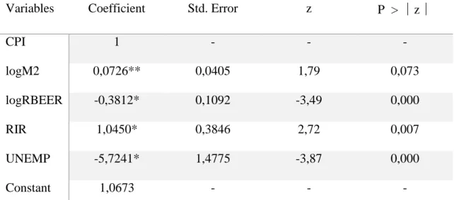
The long-run co-integrated equation is portrayed in table 5, which shows that every explanatory variable selected for this study is significant in explaining the evolution of Brazilian inflation (as measured by CPI) over the long-term. While money supply (as measured by M2) is only statistically significant at the 10% level, the remaining independent variables (real broad effective exchange rate, real interest rate and unemployment) all achieve statistical significance at the more conservative 1% level. Apart from this, we can additionally verify that their long-run relationship with inflation goes alongside with what is conveyed in relevant literature, with one exception – the real interest rate. Since every variable in this study has values that are either percentages or logarithmic in form, we can proceed with interpreting the results as a matter of elasticity. As such, a percentage increase in the money supply and the real interest rate generates an increase in the value of inflation of approximately 0,073 percent and 1,045 percent, respectively (ceteris paribus). On the other hand, an increase of one percent in unemployment
14 and the real broad effective exchange rate (i.e. an appreciation of one percent) leads to a decrease in the value of inflation of 5,724 percent and 0,381 percent, respectively (ceteris paribus).
In the next four paragraphs I intend to clarify the economic rationale behind why these long-run relationships are verified in Brazil and do so with the intention of subsequently deriving policy implications for the country, which can be found in the concluding section of this paper.
- Money supply: Increasing the amount of liquidity that is available in Brazil at a faster pace than the growth in real gross domestic product leads to inflation because there is a greater amount of money running after a relatively smaller amount of goods – even if the amount of goods increases from one period to the next, individuals register an even higher increase in their income and thus are more likely to go ahead and spend it; since suppliers cannot immediately respond to this increased demand, they push up their prices in order to reach a new equilibrium. This represents an increase in aggregate demand that is not equally matched (or surpassed) by an increase in aggregate supply and thus generates demand-pull inflation.
- Real broad effective exchange rate: A depreciation in Brazil’s real broad effective exchange rate reduces its competitiveness when compared against other countries, thus making imports more expensive and exports cheaper. While the former causes inflation in a straightforward cost-push fashion (due to the higher cost of foreign goods) and shifts domestic aggregate demand for imports towards domestically produced goods (generating demand-pull inflation), the latter leads to higher foreign demand for Brazilian goods, which exerts pressure in Brazilian suppliers and eventually translates into demand-pull inflation. - Real interest rate: Brazil appears to contradict the well-documented and predominant
15 rates make both individuals and businesses less willing to borrow money and, as such, contribute to an overall reduction in aggregate demand. The opposite is verified in Brazil. A possible explanation for this phenomenon is linked with the fact that the Brazilian real interest rate enjoyed a downward trend since the mid-2000s up until 2013, while inflation remained relatively stable during the same period (see figure 1). Given that this period encompasses the majority of this study’s sample used in the estimation of the vector error correction model and corresponding long-run co-integration equation, this relationship is likely to be confined to the aforementioned decade or to a slightly longer period.
- Unemployment: The relationship between unemployment and inflation in Brazil seems to follow the dynamics specified in the Philips curve – a higher demand for labor will drive inflation upwards, and vice-versa. If the country is growing and high employment is the norm – with individuals receiving either stable or rising incomes –, banks also become more willing to lend money in higher volumes and at cheaper prices, thus stimulating an increase in aggregate demand and causing demand-pull inflation.
The specification of the vector error correction model estimated can be found in table 6. The error correction term presents a negative sign and is statistically significant at the 5% level, which serves to confirm that the variables included in the model enjoy a long-run equilibrium relationship towards which they are adjusted at the speed of 6,18% per period after eventual short-run deviations. Next, we can proceed with the assessment of the short-run dynamics between the variables. We start by observing that past inflation has a negative and significant impact on its current value, which seems to point towards policy effectiveness in the sense that, when inflation starts to pick up and achieve higher-than-preferred values, actions from entities such as the Brazilian Central Bank appear able enough to curb this behavior. When it comes to money supply, we can verify the existence of two statistically significant short-run relationships with inflation that contradict each other (i.e. have opposite signs) – if an increase in money
16 supply is associated with lower inflation in a particular quarter, it is followed by a correction in the following period that drives inflation upwards. Regarding the real broad effective exchange rate, we can also observe a significant short-run dynamic since an appreciation in the Brazilian currency will drive inflation down, just as expected. The real interest rate appears to follow a similar short-run interaction to that of the money supply, given that if in one quarter it is associated with a decrease in inflation, in the next it will verify the opposite. Finally, unemployment also appears to be an important variable in explaining inflation in the short-term but, as opposed to the behavior presented by both the money supply and the real interest rate, it always has the same effect on the current value of inflation – if unemployment increases, inflation will decrease in the future (and vice-versa).
Table 5: Long-run Co-integrated Equation
In the following table, * and ** denote statistical significance at the 1% and 10% levels, respectively.
Variables Coefficient Std. Error z P > │z│
CPI 1 - - - logM2 0,0726** 0,0405 1,79 0,073 logRBEER -0,3812* 0,1092 -3,49 0,000 RIR 1,0450* 0,3846 2,72 0,007 UNEMP -5,7241* 1,4775 -3,87 0,000 Constant 1,0673 - - -
17 Table 6: Vector Error Correction Model
In the following table, LD refers to 1-quarter lag, L2D to 2-quarter lag, L3D to 3-quarter lag and L4D to 4-quarter lag. Additionally, *, ** and *** denote statistical significance at the 1%, 5% and 10% levels, respectively.
Regressors Coefficient Std. Error z P > │z│
Error Corr. Term -0,0618** 0,0301 -2,05 0,040
LD.CPI 0,1463 0,3609 0,41 0,685 L2D.CPI 0,4616 0,3826 1,21 0,228 L3D.CPI -0,8824** 0,3790 -2,33 0,020 L4D.CPI 0,1372 0,2780 0,49 0,622 LD.logM2 0,1216** 0,0569 2,14 0,033 L2D.logM2 -0,1872** 0,0882 -2,12 0,034 L3D.logM2 0,1271 0,0830 1,53 0,126 L4D.logM2 -0,1061 0,0866 -1,22 0,221 LD.logRBEER 0,0187 0,0355 0,53 0,599 L2D.logRBEER -0,0029 0,0258 -0,11 0,911 L3D.logRBEER -0,0328*** 0,0190 -1,73 0,084 L4D.logRBEER -0,0153 0,0166 -0,92 0,357 LD.RIR -0,2691 0,2164 -1,24 0,214 L2D.RIR 0,4762*** 0,2595 1,84 0,066 L3D.RIR -0,9814* 0,2735 -3,59 0,000 L4D.RIR 0,2369 0,2683 0,88 0,377 LD.UNEMP 0,1978 0,2614 0,76 0,449 L2D.UNEMP -0,6980** 0,3046 -2,29 0,022
18 L3D.UNEMP 0,0677 0,2786 0,24 0,808 L4D.UNEMP -0,5584** 0,2658 -2,10 0,036 Constant 0,0045*** 0,0026 1,68 0,092 R Squared 0,8816 RMSE 0,0046 Chi2 163,8712 P > Chi2 0,0000 Log Likelihood 827,3826 Diagnostic Tests
To investigate whether the residuals of the aforementioned vector error correction model suffer from autocorrelation, I employ the Lagrange-multiplier test, which states as its null hypothesis that there is no autocorrelation at a particular lag order. Examining table 7 leads to the conclusion that, since the probability values for every lag order are above the 5% level, we cannot reject the null hypothesis and thus are not in the presence of autocorrelation.
Regarding the distribution of the residuals, the Jarque-Bera test is used to test for normality and its null hypothesis specifies that the residuals follow a normal distribution. The results can be observed in table 8. Once more, given that our target equation is associated with a probability of over 5%, we cannot reject the null hypothesis and as such can infer that the residuals are normally distributed.
Table 7: Lagrange-multiplier Test Results
Lag Chi2 Degrees of Freedom Prob. > Chi2
19
2 23,9408 25 0,52280
3 20,8998 25 0,69818
4 19,2790 25 0,78355
5 16,8047 25 0,88875
Table 8: Jarque-Bera Test Results
Equation Chi2 Degrees of Freedom Prob. > Chi2
∆CPI 0,552 2 0,75885
Out-of-sample Performance
The ranking of the top five short-run Brazilian CPI forecasters is selected by the Brazilian Central Bank accounting for “the accuracy of one-month forecasts over the last six months”. As such, the residuals accounted for in this ranking are not directly comparable to the ones obtained in this paper’s out-of-sample forecast, given that the latter are only obtained once for every quarter while the former are computed six times for a period of six months. We can nevertheless still find a decent proxy in these professional forecasts if we divide their residuals in half, however we must keep in mind that this essentially converts a six-month period into a three-month period, and not a monthly periodicity into a quarterly one.
With this information in mind, I reach a relative root mean squared error of 0,3639 by dividing the root mean squared error computed with the residuals obtained with this paper’s vector error correction model (0,0100) by the one computed with the residuals of the aforementioned top professional forecast (0,0273). Since a value below 1 is obtained, we can infer that our model is well fitted and presents adequate performance out-of-sample.
20 V. Conclusion
This study attempted to dissect Brazilian inflation with the goal of achieving a clearer picture of its dynamics for both the short and long-run. To that end, I conducted several empirical tests and estimated a vector error correction model over the period between 2002 and 2018. Every independent variable selected – money supply, real broad effective exchange rate, real interest rate and unemployment – was found to be statistically significant to the explanation of short and long-term inflation movements, and evidence suggests that both demand-pull and cost-push phenomena play crucial roles in determining Brazilian inflation.
The monetary policy of the Brazilian Central Bank appears to be effective in controlling inflation over the short-term, given the statistically significant and negative relationship between past and current inflation, which is also indicative of the inconsequential role that public inflation expectations play in the country – otherwise this interaction would be reversed. Money supply contributes to both upward and downward inflationary pressures in the short-run, thus making its long-run impact more relevant from a research and policy perspective – the latter conforms to the traditional monetarist view that an increase in the amount of money circulating in the economy will contribute to rising inflation, hence variations in money supply become a key point of consideration for Brazilian authorities over the long-term in the sense that there should be an effort to keep them in line with the growth in real gross domestic product and to avoid any unnecessary monetary expansions.
The real broad effective exchange rate also reveals adherence to the findings of relevant literature in both the short and long-run, since a depreciation in the Brazilian currency leads to higher inflation in each case, which essentially confirms that domestic inflation is influenced by foreign variables. The Brazilian Central Bank appears to be aware of this relationship and, in recent years, has often intervened in the foreign exchange market through the sale and
21 purchase of foreign exchange swaps in an effort to curb both currency volatility and depreciation.
Findings suggest that the real interest rate was not an effective tool for controlling inflation during the sample period, given that inflation followed in its footsteps instead of in the opposite direction. As mentioned in the results and discussion section, this is very likely a phenomenon observed within the boundaries of that decade and, as such, poses an intriguing question for further research with an updated data sample – is this unusual interaction still verified post-2014 or was it only a decade-long phenomenon? Additionally, another interesting topic for future research is related with the effectiveness through which the official nominal interest rate (Selic) established by the Brazilian Central Bank leaks onto the real interest rate, which will allow for a deeper understanding of the degree of influence the entity can exert over inflation movements through this particular channel.
Unemployment significantly impacts inflation in the short a long-run, and evidence points to this relationship following the principles portrayed by the Philips curve – whenever unemployment is high, inflation is low (and vice-versa). Furthermore, over the long-run and of all the variables studied in this paper, it is unemployment which exerts the biggest influence on inflation, since if the former registers an increase (decrease) of only one percent the latter will be driven downwards (upwards) approximately 5,72 percent. That being said, it becomes evident that it is extremely vital to keep unemployment under close examination in Brazil and that significant shocks to this variable should be prevented by all means.
Finally, while short-run deviations from the long-run equilibrium relationship verified between the variables in this study are adjusted every quarter, this occurs at a very sluggish pace and will take several periods to completely manifest itself. This implies that short-run shocks to inflation are likely to be felt for many periods into the future.
22 References
Arize, Chuck A. & Malindretos, John & Nippani, Srinivas. 2004. “Variations in Exchange Rates and Inflation in 82 Countries: An Empirical Investigation.” The North American Journal
of Economics and Finance, 15(2): 227-247.
Devereux, Michael. 1989. “A Positive Theory of Inflation and Inflation Variance.” Economic
Inquiry, 27(1): 105-116.
Dwyer, Gerald P. & Hafer, Rik W. 1988. “Is Money Irrelevant?” Federal Reserve Bank of
St. Louis Review, 70(3): 1-17.
Friedman, Milton. 1956. Studies in the Quantity Theory of Money. Chicago: University of Chicago Press.
Hooker, Mark A. 2002. “Are Oil Shocks Inflationary? Asymmetric and Nonlinear Specifications versus Changes in Regime.” Journal of Money, Credit and Banking, 34(2): 540-561.
Khan, Rana E. A. & Gill, A. R. 2010. “Determinants of Inflation: A Case of Pakistan (1970-2007).” Journal of Economics, 1(1): 45-51.
Laryea, Samuel A. & Sumaila, Ussif R. 2001. “Determinants of Inflation in Tanzania.” Chr.
Michelsen Institute – Development Studies and Human Rights, 12: 1-17.
Lim, Cheng H. & Papi, Laura. 1997. “An Econometric Analysis of the Determinants of Inflation in Turkey.” IMF Working Paper, 170: 1-32.
Lim, Yen C. & Sek, Siok K. 2014. “An Examination on the Determinants of Inflation.”
23 Lucas, Robert E. 1980. “Two Illustrations of the Quantity Theory of Money.” American
Economic Review, 70(5): 1005-1014.
Odusanya, Ibrahim A. & Atanda, Akinwande A. 2010. “Analysis of Inflation and Its Determinants in Nigeria.” Pakistan Journal of Social Sciences, 7(2): 97-100.
Pahlavani, Mosayeb & Rahimi, Mohammad. 2009. “Sources of Inflation in Iran: An Application of the ARDL Approach.” International Journal of Applied Econometrics and
Quantitative Studies, 6(1): 61-76.
Phillips, A. W. 1958. “The Relation Between Unemployment and the Rate of Change of Money Wage Rates in the United Kingdom, 1861–1957” Economica, 25: 283-299.
Tillmann, Peter. 2008. “Do Interest Rates Drive Inflation Dynamics? An Analysis of the Cost Channel of Monetary Transmission.” Journal of Economic Dynamics and Control, 32(2): 2723-2744.