António Afonso Ana Sofia Nunes

(1)

Carlos Pestana Barros & Nicolas Peypoch

A Comparative Analysis of Productivity Change in Italian and Portuguese Airports

WP 006/2007/DE _________________________________________________________

António Afonso & Ana Sofia Nunes

Economic forecasts and sovereign yields*

WP 02/2013/DE/UECE _________________________________________________________

De pa rtme nt o f Ec o no mic s

W

ORKING

P

APERS

ISSN Nº 0874-4548

School of Economics and Management

(2)

Economic forecasts and sovereign yields

*

António Afonso

$ #

and Ana Sofia Nunes



December 2012

Abstract

The European Commission releases twice a year economic forecasts for some macro and fiscal variables (GDP growth rate, inflation, budget balance, among others). In our research we will try to understand if the corrections made to these forecasts have an impact in sovereign yields. We will perform an econometric analysis in a panel of 15 EU countries (Austria, Belgium, Germany, Denmark, Spain, Finland, France, United Kingdom, Greece, Ireland, Italy, Luxembourg, Netherlands, Portugal and Sweden), covering the period from 1999:1 until 2012:1, and after we analyse each country individually, on the basis of a SUR analysis. We find that corrections in the EC’s forecasts do impinge on the 10-year sovereign bond yields, particularly corrections in fiscal variables, but this impact is different across countries, being more pronounced in countries with less favourable economic conditions.

Keywords:macro forecasts, fiscal forecasts, sovereign yields. JEL: C23, E44, H68.

*

The authors are grateful to Patrícia Martins for very useful comments. The opinions expressed herein are those of the authors and do not reflect those of the ECB or the Eurosystem.

$_{ISEG/UTL - Technical University of Lisbon, Department of Economics; UECE}_–_{Research Unit on Complexity and}

Economics. UECE is supported by FCT (Fundação para a Ciência e a Tecnologia, Portugal), email: aafonso@iseg.utl.pt.

#_{European Central Bank, Directorate General Economics, Kaiserstraße 29, D-60311 Frankfurt am Main, Germany.} 

(3)

Since 1998 the European Commission (EC) releases in a regular basis twice a year, in the spring and in autumn, short-term economic forecasts for the member states of the Economic and Monetary Union (EMU), candidate countries and other important economies, as the United States, Japan and the United Kingdom. The main purpose is for the checking of the Stability and Growth Pact rules (budget balance ratio higher than -3% and public debt-to-GDP ratio lower than 60%). However, since the forecasts are publicly available, investors may use this information to decide their investment portfolio, notably their investment in the sovereign bonds.

Therefore, the release of these forecasts should, theoretically, have an impact on sovereign spreads. Indeed, we may argue that rational investors use all the available information, thus a release of new information will cause a rearrangement in their investment portfolio. Favourable forecasts (higher real GDP growth, lower public debt, lower unemployment, etc.) should bring sovereign yields down, as more investors are interested in buying bonds of that particular country due to the lower risk of default. The opposite situation should also occur with unfavourable forecasts.

However, it is not obvious that this happens in reality, notably whether investors indeed rearrange their portfolios accordingly. Hence, we are interested in assessing what is the impact of releasing economic forecasts on the sovereign yields. If, as expected, the impact on sovereign yields is significant, the institutions which release these forecasts (EC, Organization for Economic and Co-operation Development (OECD), European Central Bank (ECB), and others) and in particular the governments, want to be aware of the consequences of forecast accuracy. That is particularly relevant regarding forecasts for current and next year (the ones with most obvious possible influence), but also for past years, as there are often corrections to past data. These corrections are mainly due to two possible situations: on the one hand, forecasts made by the EC are based on the information provided by the country’s government, and there may be incentives to provide some biased information;1 on the other hand, these forecasts depend on the economic situation, which is unstable, especially in times of recession. Thus, it is vital to understand the impact of these forecasts corrections on the costs of the countries’ sovereign financing.

1

(5)

Moreover, there is also an interest for private agents to know the impact of macro and fiscal forecasts, especially traders, as every anticipation of future movements in bond’s prices may bring profit. Therefore, knowing if and how the bond market reacts to the release of these forecasts is paramount.

The present research will try to provide an answer for this problem, and it is a contribute to the literature since these linkages have not been much explored, at least to our knowledge, after reading the existing related literature. In fact, there are only a few studies for the USA2, and some were made 15 or more years ago.3 On the contrary, there are numerous studies on sovereign spreads’ determinants, on forecasts’ accuracy, and on the causes of forecast errors.

We perform an econometric analysis of the linkages between different economic forecasts and sovereign yield spreads, using a panel of 15 EU countries (Austria, Belgium, Germany, Denmark, Spain, Finland, France, United Kingdom, Greece, Ireland, Italy, Luxembourg, Netherlands, Portugal and Sweden), covering the period from 1999:1 until 2012:1. First we do the analysis for the entire panel, and afterwards we study each country individually, specifically on the basis of a SUR analysis. Notice that we use as variables the difference between the forecasts of two consecutive semesters, and not the forecast itself. This has as purpose to identify not only the impact of the forecasts’ corrections in the yields, but also the credibility of the previsions.

In a nutshell, we can draw an important conclusion from our study: corrections in the EC’s forecasts do impinge on the 10-year sovereign bond yield spreads, particularly the corrections in fiscal variables (public debt and budget balance), but this impact is different across countries, being more pronounced in countries with less favourable economic conditions.

This dissertation is organised as follows. Section two covers the related literature. Section three explains and discusses the data and the construction of the variables. Section four presents the empirical strategy and the results. Section five summarises the conclusions.

2

See Canzoneri, Cumby and Diba (2003). 3

(6)

2. Literature review

2.1. Literature on sovereign spreads’ determinants

To perform our analysis, we need to know the main determinants of sovereign bond yield spreads. There is a great amount of literature on this subject, but there are still some conflicting results, as there are many factors which may influence sovereign spreads. The economic cycle, the countries’ characteristics and credibility, the investors risk aversion, and so on, can be difficult to include in the empirical analysis, and may cause econometric problems, which can bias the results or make them inconsistent.

However, there are some conclusions that are common to the majority of the studies. The variables which more often appear as significant are the level of GDP, GDP per capita or GDP growth rate (Hilscher and Nosbusch, 2010; Afonso, 2010), fiscal performance , through public debt and budget balance (Dell’Erba and Sola, 2011; Baldacci and Kumar, 2010; Afonso, Arghyrou and Kontonikas, 2012; Afonso, 2010; Amira, 2004; Laubach, 2009; Akitoby and Stratmann, 2006; Gruber and Kamin, 2010), current account balance (Amira, 2004) and monetary policy (Gruber and Kamin, 2010). The literature also presents several interesting conclusions. For example, the impact of the level of public debt is quantitatively lower than the one of public deficits (Faini, 2006; Laubach, 2009), the effects of global shocks appear to be greater than domestic factors (Faini, 2006; Ardagna, Caselli and Lane, 2004) and global risk aversion significantly affects sovereign spreads in developed countries (Bernoth, von Hagen and Schuknecht, 2012). Moreover, it is also reported that worst fiscal behaviour lowers the ratings of sovereign debt (Afonso & Gomes, 2010), which may induce a rise in the yields demanded by market participants.

(7)

They also report that financial markets distinguish between cuts in public spending, and changes in investment and in revenues. A reduction in current spending is preferred to a reduction in investment, and adjustments in revenues are more valued than those in spending, while financing by revenues is favoured over debt issuing.

A study by the EC (2011) finds a negative relationship between the strength of rules-based fiscal governance and sovereign spreads, using the Fiscal Rules Index as a measure of the quality of the fiscal institutions. Alexopoulou, Bunda and Ferrando (2009) conclude that the current account and budget balance, inflation, exchange and short-term interest rates, among other factors, influence the cost of long-term finance of new EU countries, while Afonso and Rault (2010) conclude that the inflation rate, budget and external imbalances have an impact on OECD countries sovereign spreads.

Thus, our empirical analysis will consider as determinants of the 10-year government bond yields the GDP real growth rate, the public debt-to-GDP ratio, the budget balance ratio, the inflation rate, given by the harmonised index of consumer prices (HICP), the real effective exchange rate (more specifically, the percentage change to the preceding year), the current account balance, also as a percentage of GDP (all of these sourced as EC forecasts), the international risk (represented by the VIX – the S&P 500 implied stock market volatility index), and monetary policy (represented by the short-term interest rates defined by the monetary authority). We also control for the existence and strength of fiscal rules, including as a variable the Fiscal Rude Index, calculated by the EC.

2.2. Literature on forecast errors

Regarding forecasts errors, there are two different topics usually explored: errors in government’s forecasts and their causes, and errors in independent agencies’ forecasts and their causes. Both are important for our work due to the dependency of the EC’s forecasts on governments’ forecasts, as stated above.

Concerning governments’ forecasts, three main conclusions appear in the literature: 1) preliminary data releases are biased and non-efficient predictors of the true

(8)

2006; Merola and Pérez, 2012; Martins and Mora, 2007; Frankel, 2011; Jonung and Larch, 2006);

2) the economic cycle is not fully included in the GDP forecast, making GDP forecast errors an important cause of budget deficit errors (Merola and Pérez, 2012; Frankel, 2011; Jonung and Larch, 2006; Moulin and Wierts, 2006; Castro, Pérez and Vives, 2011);

3) being subject to a fiscal rule, without having strong and independent supervision, leads to an increase in GDP and budget deficit errors, possibly due to creative accounting (von Hagen and Wolff, 2006; Frankel, 2011).

Bernoth and Wolff (2008), and von Hagen and Wolff (2006) mention that most European Union’s members incur in stock flow adjustments (i.e., the change in their government debt is higher than the budget deficit), which increases the yields demanded by financial markets. This increase is higher when the events of creative accounting are reported in the media. On the other hand, Castro, Pérez and Vives (2011) argue that modifications in Eurostat budget rules also explain a significant part of forecast errors, and forecasts may be considered rational after two years (i.e., forecast for year t may be considered correct in year t+2). This conclusion was the reason for the use in our study of forecast’s corrections till two years ago as regressors. Finally, elections and good economic cycles tend to increase the optimism in forecasts (Merola and Pérez, 2012; Frankel, 2011; Castro, Pérez and Vives, 2011).

Concerning independent agencies’ forecasts, two main conclusions are possible: 1) they seem to be unbiased and efficient, either for the EU and for the non-EU

countries (Grenouilleau, Melander and Sismanidis, 2007);

2) however, they appear to be correlated with the electoral cycles, though less than those from the government, and do not include all the available information, though they consider more information than governments (Merola and Pérez, 2012).

(9)

or for the budget balance. They also conclude that forecasts errors are greater in the case of the ones from the International Monetary Fund (IMF), then in the one from the EC and, finally, in the OECD. However, they argue that this can be due to the time of the release of the forecasts. Indeed, the IMF’s ones are the first to be published in the year, followed by the EC’s and after by the OECD’s.

In our analysis we will consider EC’s forecasts, as they are part of the basis of budgetary surveillance in the context of the application of the Excessive Deficits Procedure, and are considered more reliable than the government’s, being a major reference for investors, economists and managers.

3. Data and variables

As already mentioned, in our study we use a panel of 15 countries: Austria (AT), Belgium (BE), Germany (DE), Denmark (DK), Spain (ES), Finland (FI), France (FR), United Kingdom (GB), Greece (GR), Ireland (IE), Italy (IT), Luxemburg (LU), Netherlands (NL), Portugal (PT) and Sweden (SE).

The EC’s forecasts of budget balance-to-GDP ratio (BAL), public debt-to-GDP ratio (DEBT), GDP real growth rate (YR), current account balance (CA), inflation (INF) and real effective exchange rate (REER) were retrieved from the EC’s website, as well as the short-term interest rates (I), the 10-year government bond yields (YIELDS) and the fiscal rule index (FRI). The VIX was obtained from Bloomberg’s.

The forecasts are released twice a year, typically around March-April (the spring forecast) and October-November (the autumn forecast), therefore, our data will be bi-annual.4 As the first forecasts were made in the second semester of 1998, our analysis covers the period from 1999:1 till 2012:1. The short-term interest rates, the yields and the VIX used relate to the month of the release of the forecast. For example, the spring 2012 EC’s forecasts were released on May 11th, thus we use the short-term rate, yield and VIX observed in May (notice that for the VIX we calculate the monthly average, using the daily values). We use monthly yields instead of daily ones in order to try to capture some market anticipation of the forecast’s release.

It is important to understand correctly the meaning of all variables. We will include forecasts made in year t for year t, year t+1, and also the estimations made for years t-1

4

(10)

and t-2. This choice was based on Castro, Pérez and Vives (2011), as mentioned above. If forecasts may be considered rational after two years, investors will not pay much attention to corrections made after that (except if those corrections are truly significant, but it is not a frequent occurrence). Moreover, as already said, we will use forecasts’ corrections as variables, and not the forecast itself.

Therefore, every semester s we have a forecast for variable X, for country i and year

t, Xti,s. Our variable of interest will then be ΔXti,s = Xti,s - Xti,s-1, the difference between forecasts made for year t in two consecutive semesters. We are not interested in knowing if the release of the forecast itself has an impact on the yield (this would be simply studying the determinants of the yields), but whether if the corrections made in the forecasts are significant enough to alter the yields. This way, we can evaluate if the EC’s and governments forecasts have credibility.

For better understanding the mechanics of building these variables, we can see the following example:

In March 2005 (semester 13) the spring’s forecasts were released. Our variables are:

 ΔXt

i,s = X2005i,13 – X2005i,12, the difference between the forecast made in semester 13 (2005 spring forecast) for the value of variable X in 2005 and the forecast made in semester 12 (2004 autumn forecast) also for year 2005;

 ΔXt+1

i,s = X2006i,13 – X2006i,12, the difference between the forecast made in semester 13 (2005 spring forecast) for X in 2006 and the forecast made in semester 12 (2004 autumn forecast) for X in 2006;

 ΔXt-1

i,s = X2004i,13 – X2004i,12, the difference between the estimation made in semester 13 (2005 spring forecast) for X in 2004 and the estimation made in semester 12 (2004 autumn forecast) for X in 2004;

 ΔXt-2

i,s = X2003i,13 – X2003i,12, the difference between the estimation made in semester 13 (2005 spring forecast) for X in 2003 and the estimation made in semester 12 (2004 autumn forecast) for X in 2003.

For the 2005 autumn forecast, since we remain in the same year, the meaning of the variables is similar (ΔXt

(11)

made in semester 14 (November, 2005 autumn forecast) and those made in semester 13 (March 2005). Although the frequency of our data is bi-annual, we always have to centre the dating to the year in which it has been done, in order to know to which year the forecast refers to.

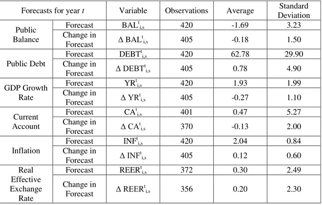
In Appendix A, tables AII, AIII, AIV and AV provide information about number of observations, average and standard deviation of all forecasts and forecasts’ corrections.

4. Empirical strategy and results

4.1. Panel estimation results

We will start by using a panel data approach, using all data to try to obtain the aggregate effect of forecasts’ corrections on the sovereign yields. The baseline specification is

(1)

where T={t, t+1, t-1, t-2} refers to the year of the forecast or estimation (we use the term “estimation” to refer to forecasts made for years t-1 and t-2), and ={BAL, CA, DEBT, INF, REER, YR} is the forecasts’ vector, and varies from regression to regression, depending on the variables we want to study.

Due to the correlation between ΔDEBT and ΔBAL, we never include them in the same regression. We excluded ΔREERt+1

as a regressor because it had too few observations. In fact, the further ahead forecast that the EC makes for this variable is just for the year following their release. So, in the first semester we do not have ΔREERt+1

, as it does not exist REERt+1i,s-1.

(12)

We use instrumental variables for ΔDEBT and ΔBAL, regarding forecasts for year t and t+1, since they are correlated with the YIELDS. Every year, governments have to make interest payments to bond owners, an expense that it is accounted for in the budget balance and, consequently, in public debt. Therefore, the higher the interest rate demanded by investors in the bond’s auction, the higher will be the budget deficit and consequently the stock of future debt. Moreover, forecasts for the fiscal variables for t and for t+1 are also likely to be influenced by the current 10-year secondary market bond yields.

Additionally, we have tested for the endogeneity of ΔYR, also for the forecasts for year t and t+1, to exclude a possible effect of the 10-year sovereign yields on the country’s economic growth. Indeed, higher yields may push public balances to critical values, forcing governments to adopt somewhat more austere programs, reducing their expenses or increasing their revenues, mostly through higher taxation. Either way, these are negative stimulus to the economy, and may have a contractionary effect on real GDP.

In order to test for endogeneity, we perform the Wu-Hausman’s endogeneity test, in which we start to estimate ΔYRt _{and ΔYR}t+1 _{in function its instruments (ΔYR}t-1

and VIX, for both). Then, we save the estimations of ΔYRt_{and ΔYR}t+1

obtained from these two regressions, and include them as regressors in the original regressions. If the estimation of ΔYRt

is significant (p-value lower than 0.10), then ΔYRt is endogenous and the use of ΔYRt-1

and VIX as instruments is needed. The same happens with ΔYRt+1

.

(13)

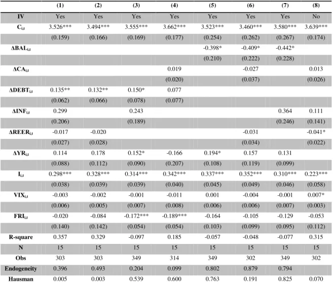
Table I – Estimation results for 10-year yields: forecasts for year t

(1) (2) (3) (4) (5) (6) (7) (8)

IV Yes Yes Yes Yes Yes Yes Yes No

Ci,t 3.526*** 3.494*** 3.555*** 3.662*** 3.523*** 3.460*** 3.580*** 3.639*** (0.159) (0.166) (0.169) (0.177) (0.254) (0.262) (0.267) (0.174)

ΔBALi,t -0.398* -0.409* -0.442*

(0.210) (0.222) (0.228)

ΔCAi,t 0.019 -0.027 0.013

(0.020) (0.037) (0.026)

ΔDEBTi,t 0.135** 0.132** 0.150* 0.077 (0.062) (0.066) (0.078) (0.077)

ΔINFi,t 0.299 0.243 0.364 0.111

(0.206) (0.189) (0.246) (0.141)

ΔREERi,t -0.017 -0.020 -0.031 -0.041*

(0.027) (0.028) (0.034) (0.022)

ΔYRi,t 0.114 0.178 0.152* -0.166 0.194* 0.157 0.131

(0.088) (0.112) (0.090) (0.207) (0.108) (0.119) (0.099)

Ii,t 0.298*** 0.328*** 0.314*** 0.342*** 0.337*** 0.352*** 0.310*** 0.223*** (0.038) (0.039) (0.039) (0.040) (0.045) (0.049) (0.046) (0.058)

VIXi,t -0.003 -0.002 -0.001 -0.011 0.001 -0.004 -0.001 0.007*

(0.006) (0.005) (0.007) (0.008) (0.006) (0.006) (0.007) (0.003)

FRIi,t -0.020 -0.084 -0.172*** -0.189*** -0.164 -0.105 -0.129 -0.053

(0.140) (0.142) (0.054) (0.054) (0.103) (0.099) (0.095) (0.112)

R-square 0.357 0.329 -0.097 0.185 -0.057 -0.048 -0.077 0.315

N 15 15 15 15 15 15 15 15

Obs 303 303 349 314 349 302 349 302

Endogeneity 0.396 0.493 0.204 0.099 0.802 0.879 0.794

Hausman 0.005 0.003 0.539 0.600 0.763 0.191 0.825 0.070

Note: the asterisks *, ** and *** represent significance at 10, 5 and 1% level, respectively. The values present between parenthesis are the standard error. IV indicates if instrumental variables were used in the regression, N is the number of countries included in the sample, Obs is the number of observations, Endogeneity is the p-value obtained by performing the Wu-Hausman endogeneity test for ΔYR, and Hausman is the p-value for the Hausman’s random effect test.

(14)

Table II – Estimation results for 10-year yields: forecasts for year t+1

(1) (2) (3) (4) (5) (6) (7) (8)

IV Yes Yes Yes Yes Yes Yes Yes No

Ci,t 3.581*** 3.664*** 3.633*** 3.681*** 3.881*** 3.843*** 3.795*** 3.629*** (0.207) (0.224) (0.203) (0.202) (0.378) (0.405) (0.314) (0.166)

ΔBALi,t+1 -0.456* -0.334* -0.373*

(0.259) (0.198) (0.209)

ΔCAi,t+1 0.028 0.061 0.056**

(0.018) (0.038) (0.027)

ΔDEBTi,t+1 0.099* 0.085* 0.094* 0.085* (0.053) (0.052) (0.050) (0.051)

ΔINFi,t+1 0.200 0.190 0.207 -0.024

(0.164) (0.140) (0.170) (0.063)

ΔREERi,t -0.036 -0.038 -0.047 -0.039*

(0.029) (0.031) (0.037) (0.021)

ΔYRi,t+1 0.048 0.020 0.098 -0.004 0.185 -0.017 0.106

(0.101) (0.106) (0.092) (0.097) (0.178) (0.179) (0.168)

Ii,t 0.335*** 0.342*** 0.323*** 0.334*** 0.328*** 0.310*** 0.293*** 0.244*** (0.048) (0.048) (0.047) (0.046) (0.051) (0.050) (0.054) (0.043)

VIXi,t -0.011 -0.011 -0.004 -0.010 -0.013 -0.016 -0.008 0.006*

(0.009) (0.010) (0.008) (0.010) (0.014) (0.013) (0.010) (0.003)

FRIi,t -0.006 -0.173** -0.157 -0.177*** -0.225** -0.150 -0.130 -0.076

(0.192) (0.069) (0.171) (0.051) (0.089) (0.120) (0.206) (0.106)

R-square 0.302 0.197 0.234 0.215 -0.412 -0.186 -0.131 0.319

N 15 15 15 15 15 15 15 15

T 303 303 349 314 349 302 349 302

Endogeneity 0.945 0.924 0.728 0.295 0.466 0.628 0.697

Hausman 0.001 0.103 0.089 0.231 0.101 0.169 0.028 0.000

Regarding the forecasts for the next year, in Table II, when the public debt ratio increases by 1 p.p., yields go up, in average, 0.091 p.p., and when budget balance increases in 1 p.p., yields go down 0.388 p.p., in average. Current account balance corrections appear as significant in one of the regressions, having a positive but smaller impact (0.056) than the fiscal variables. The constant term, short-term interest rate and FRI are significant again.

(15)

comparing to budget balance. The constant term, short-term interest rate and VIX remain significant, and VIX starts to appear as well.

Table III - Estimation results for 10-year yields: estimations for year t-1

(1) (2) (3) (4) (5) (6) (7) (8)

IV No No No No No No No No

Ci,t 3.642*** 3.647*** 3.691*** 3.624*** 3.681*** 3.631*** 3.692*** 3.641***

(0.159) (0.154) (0.193) (0.156) (0.168) (0.172) (0.175) (0.167)

ΔBALi,t-1 -0.211** -0.283*** -0.212**

(0.090) (0.102) (0.091)

ΔCAi,t-1 -0.042 -0.053 -0.042

(0.028) (0.044) (0.041)

ΔDEBTi,t-1 0.076 0.077 0.073 0.074 (0.049) (0.048) (0.052) (0.050)

ΔINFi,t-1 -0.133 0.138 0.168 -0.348

(0.417) (0.312) (0.301) (0.369)

ΔREERi,t-1 0.004 0.004 0.000 0.010

(0.098) (0.098) (0.104) (0.101)

ΔYRi,t-1 -0.137 -0.137 -0.054 -0.134 -0.052 -0.149 -0.058

(0.129) (0.128) (0.079) (0.106) (0.084) (0.131) (0.086)

Ii,t 0.273*** 0.272*** 0.271*** 0.269*** 0.262*** 0.280*** 0.261*** 0.241***

(0.034) (0.033) (0.032) (0.032) (0.036) (0.033) (0.037) (0.045)

VIXi,t 0.002 0.002 0.005 0.004 0.006* 0.003 0.006* 0.006**

(0.003) (0.003) (0.004) (0.003) (0.003) (0.003) (0.003) (0.003)

FRIi,t -0.124 -0.122 -0.212*** -0.132 -0.191* -0.165 -0.194* -0.127

(0.095) (0.094) (0.061) (0.096) (0.113) (0.048) (0.113) (0.099)

R-square 0.355 0.354 0.228 0.331 0.289 0.259 0.289 0.293

N 15 15 15 15 15 15 15 15

T 304 304 349 311 349 302 349 302

Hausman 0.072 0.046 0.610 0.298 0.261 0.210 0.259 0.045

(16)

which inflation appears as significant, its coefficient is 0.729, probably due to the fact that higher inflation reduces the real value of debt.

We find once more that the constant term, short-term interest rate and FRI are significant, as in all the tables above. Moreover, in this case VIX is also significant in all regressions, probably because investors do not pay attention to corrections in forecasts of so far back, thus VIX gains significance.

Table IV - Estimation results for 10-year yields: estimations for year t-2

(1) (2) (3) (4) (5) (6) (7) (8)

IV No No No No No No No No

Ci,t 3.547*** 3.549*** 3.669*** 3.629*** 3.662*** 3.577*** 3.677*** 3.613***

(0.134) (0.134) (0.176) (0.160) (0.156) (0.147) (0.160) (0.161)

ΔBALi,t-2 -0.122 -0.415 -0.129

(0.348) (0.448) (0.348)

ΔCAi,t-2 -0.094** -0.129** -0.125

(0.042) (0.060) (0.078)

ΔDEBTi,t-2 0.206 0.206 0.165 0.203 (0.146) (0.145) (0.130) (0.148)

ΔINFi,t-2 -1.132 0.275 0.729*** -0.931

(1.156) (0.340) (0.214) (1.113)

ΔREERi,t-2 -0.042 -0.043 -0.063 0.008

(0.075) (0.075) (0.073) (0.093)

ΔYRi,t-2 -0.331 -0.329 -0.195** -0.188 -0.222* -0.398 -0.251**

(0.201) (0.200) (0.098) (0.167) (0.119) (0.259) (0.118)

Ii,t 0.243*** 0.243*** 0.263*** 0.242*** 0.240*** 0.238*** 0.241*** 0.214***

(0.033) (0.033) (0.032) (0.032) (0.039) (0.035) (0.039) (0.044)

VIXi,t 0.006* 0.006* 0.008** 0.007** 0.009*** 0.008*** 0.009*** 0.007***

(0.003) (0.003) (0.003) (0.003) (0.003) (0.003) (0.003) (0.003)

FRIi,t -0.024 -0.025 -0.214*** -0.160*** -0.190 -0.163*** -0.207* -0.032

(0.074) (0.074) (0.063) (0.052) (0.116) (0.045) (0.121) (0.078)

R-square 0.391 0.391 0.255 0.300 0.280 0.251 0.286 0.289

N 15 15 15 15 15 15 15 15

t 290 290 349 294 349 287 349 287

Hausman 0.000 0.004 0.871 0.331 0.003 0.121 0.004 0.016

(17)

Accordingly, we may say that investors pay attention to countries’ fiscal behaviour, demanding higher yields when public the debt ratio increases and the budget balance decreases (which in most cases, is an increase in public deficit), meaning investors penalize countries which engage in a expansionary fiscal policy financed by debt issuance.

Looking at the results of the different tables, we can conclude that investors pay more attention to corrections made in forecasts for current and next year than to corrections made in estimations for one and two years back. This may occur due to investor’s confidence in EC’s forecast accuracy (in fact, corrections for previous years tend to be smaller5), or a higher investor’s preference for values of fiscal variables for current and next years. In terms of policy implication, if the more accurate values are only obtained afterwards, there will only be a penalization for worst budget balances, and it will be lower than if budget balances’ data were corrected before.

The coefficient for the short-term interest rate is positive (on average, it is 0.284), meaning higher short-term rates induce higher yields. When a central bank increases these rates, it is engaging in a contractionary monetary policy, and trying to slow down or “cooling” the economy, in order to maintain price stability. As a consequence, one can expect a deceleration in economic activity, which may worsen budget balances and compromise the country’s ability to pay the debt, thus bringing the yields up.

The coefficient for the FRI is negative (on average, it is -0.190), meaning that higher values of this indicator bring the yields down. The FRI is calculated based on the Fiscal Rule Strength Index, which evaluates the quality and visibility of a country’s institutional features, essential to the correct application of the fiscal rule. The higher their quality and visibility, the higher is the probability and credibility of following the rule, thus lower are the yields demanded. If investors believe the government will oblige to the limits imposed, then there is higher credibility that fiscal imbalances will be quickly corrected.

The constant term may be interpreted as a risk premium demanded by investors, related to the probability of default. At the aggregate level, it is, on average, 3.635, but

5

(18)

as we will see ahead it differs quite a lot across countries, depending on the perceived risk attributed to each one.

Finally, real GDP growth rate forecast’s corrections are also significant for years

t and t-2. It could be expected that this variable would be as meaningful as the fiscal variables, as it is a vital indicator of a country’s economic viability and debt sustainability. In spite of its relevant value as an indicator of the state of the economy, real GDP growth rates forecasts are the most volatile6, as they depend on external and non controllable factors, among others. Hence, investors may not always react to small corrections in this variable’s forecast, as they are very frequent, or may actually anticipate some errors (for example, they may anticipate that forecasts are too optimistic). Another possible explication will be given ahead, after performing the SUR analysis. Indeed, if corrections in GDP growth rate forecasts have opposite effects in the countries’ yields, then when we estimate for the entire panel these effects may cancel each other, leading to the statistic insignificance of these corrections.

Nevertheless, an increase in real GDP growth rate forecasts for current year increases yields, but an increase on real GDP growth rate estimation for last year decreases yields. Two opposite effects seem to be at play. On the one hand, higher growth increases firm’s profits, investment returns and, consequently, stocks dividends, which makes the stock market more profitable and attractive, leading to bond selling, decrease in bond’s prices and increase in bond’s yields, in order to attract investors again (a positively sloped yield curve also tends to reflect growth expectations). On the other hand, higher growth can suggest lower debt and budget balance ratios to GDP, implying a lower probability of default, which makes the country’s sovereign bonds safer investments and, as a consequence, the yields demanded are lower.

4.2. Robustness tests

Although there are EC’s forecasts until 2012:1, the FRI only has data until 2010:2. Consequently, in the results shown above, three forecast’s releases were not included (spring and autumn of 2011, and spring of 2012). In order to overcome this problem, we did two robustness tests, to see if the results obtained were still valid: first, we added one observation to the FRI, making the value for this variable in 2011 equal to

6

(19)

the one verified in 2010; second, we removed the FRI from the sample. All econometric details (instrumental variables, random or fixed effects, YR endogeneity and White covariance matrix) remain valid, and the results are reported in Appendix B (Tables BI, BII, BIII, BIV, BV, BVI, BVII and BVIII).

Comparing the results with one extra FRI observation (see Tables BI, BII, BIII and BIV in Appendix B) with the initial baseline specification, we observe that fiscal variables still remain the most important variables among the forecasts. However, public debt increases its importance, being significant for all years (before it was only significant for years t and t+1), and the budget balance looses magnitude, as it only appears significant in forecasts for year t-1, and before it was also for years t and t+1. The real GDP growth rate never appears as significant, as well as the current account balance. On the contrary, inflation now appears as significant for years t, t+1 and t-2, when it used to be significant only for t-2, and real effective exchange rate has a significant impact, regarding forecasts for years t and t+1, like current account balance, in forecasts for year t+1.

It is also worth noting that the magnitude of the short-term interest rate impact decreases significantly. Now, an increase of 1 p.p. in this rate only pushes yields up in 0.173 p.p. (0.284 p.p., in the initial results). In contrast, FRI has a greater impact (a decrease of 0.289 p.p. in yields instead of 0.190 p.p.), as well as the constant term (the coefficient increases from 3.635 to 4.011).

Hence, adding the year 2011 to our sample allows keeping the main conclusions, but changes some of the results. This may happen due to instability and uncertainty of this year (in 2011 Portugal asked for a financial assistance, implementing the EC/ECB/IMF Economic Adjustment Programme, Greece asked for a second financial loan, Italian and Spanish bonds started to be under pressure), which lead to a bigger suspicious by the investors, not relying so much on public balance and GDP growth rate forecasts, as they tend to undergo several ex-post corrections.

(20)

now 4.165). Finally, the real effective exchange rate is significant in terms of the forecasts for years t+1 and t-2.

These results seem to confirm the idea that the instability and uncertainty of 2011 and 2012 may alter a bit the results obtained in the initial panel. The disbelief in government’s accounts led investors to overlook the budget balance corrections, as they do not believe they are very credible in that context, and start to give more importance to public debt. In addition, countries began to rely on exportations to grow, as their internal demand diminished a lot, thus real effective exchange rate increased its importance as an indicator of the country’s economic evolution.

4.3. Country estimation – SUR

In addition to our panel analysis, we have performed an individual analysis for the countries. In spite of having similar political systems, citizens’ rights and ways of life, and the fact that the majority belongs to the same monetary union (EMU), which means that monetary policy is equal to all, there are many characteristics that differ from country to country. Fiscal and labour policies are independent (governments in EMU countries only have to obey the limits imposed by SGP), the production structure varies a lot, as countries specialized on their competitive advantages due to the free trade market between European countries. Moreover, productivity levels differ.

Thus, investors may react differently to corrections in forecasts, as they give different credibility to each country. Especially after the beginning of the sovereign debt crisis, it is expected that a correction in the forecast of the level of public debt causes more impact on the Greek’s yields than on the German ones. The lower is the country’s credibility, the higher the impact of forecast’s corrections, in particular “bad” corrections (increases of budget deficits or public debt, lower GDP real growth rate, for example).

(21)

more the yields, according to the literature, but there are still many factors which may have an impact. However, many are non-measurable.

Hence, when this correlation exists, it is more efficient to estimate the system of equations with SUR than to estimate each regression with Ordinary Least Squares (OLS). We will use this model in two different specifications, due to the correlation between public debt and budget balance, as mentioned above:

(2) (3)

where T = {t, t+1, t-1, t-2} refers to the year of the forecast. From equation (2) we will create a system of fourteen regressions, one for each country (Luxembourg is excluded, because it has very few observations), and we do the same with equation (3). Once again, we separate the regressions through year of forecast, so we will have eight systems, regarding forecasts for years t, t+1 and estimations for years t-1 and t-2 for both regressions. Notice that we remove the FRI as a regressor, although it was significant in the panel. We need to do this because the FRI is a constant for Greece, and almost a constant for Belgium and Netherlands, which causes collinearity problems.

(22)

Table V - Individual results of estimations of forecasts for year t, for regression (2)

Ci,t DEBTi,t INFi,t REERi,t YRi,t Ii,t VIXi,t R-square Obs

AT 3.120*** -0.008 -0.127* -0.043 -0.095 0.415*** 0.000 0.700 24

(0.198) (0.015) (0.067) (0.031) (0.058) (0.044) (0.007)

BE 3.312*** -0.047*** 0.006 -0.080*** -0.141** 0.302*** 0.012 0.599 25 (0.208) (0.016) (0.046) (0.023) (0.057) (0.049) (0.007)

DE 2.801*** 0.018 -0.038 0.014 0.032 0.550*** -0.013 0.678 25

(0.273) (0.017) (0.074) (0.011) (0.040) (0.064) (0.010)

DK 3.568*** -0.036*** 0.343 -0.102 -0.146 0.313** 0.003 0.771 13

(0.352) (0.013) (0.323) (0.105) (0.220) (0.147) (0.031)

ES 4.013*** 0.018 0.230** -0.102** -0.194 0.117 0.005 0.283 25

(0.298) (0.047) (0.110) (0.040) (0.141) (0.078) (0.011)

FI 2.852*** 0.119*** 0.052 -0.052** 0.010 0.520*** -0.005 0.817 25

(0.189) (0.016) (0.068) (0.025) (0.035) (0.046) (0.007)

FR 3.143*** 0.038* -0.030 -0.008 0.128* 0.413*** -0.001 0.686 25

(0.199) (0.020) (0.064) (0.019) (0.070) (0.046) (0.007)

GB 3.287*** 0.056** 0.039 0.066*** 0.073 0.355*** -0.005 0.763 25

(0.242) (0.027) (0.086) (0.012) (0.097) (0.034) (0.009)

GR 9.080*** -0.256*** 0.436 -0.322 -1.082** -1.431*** 0.041 0.612 25 (1.895) (0.041) (0.420) (0.212) (0.431) (0.519) (0.066)

IE 5.799*** 0.080*** 0.571*** -0.069 0.027 -0.526*** 0.022 0.474 25

(0.658) (0.020) (0.209) (0.055) (0.111) (0.178) (0.024)

IT 3.995*** -0.016 0.208 -0.066** -0.089 0.085 0.017* 0.247 25

(0.277) (0.032) (0.127) (0.033) (0.105) (0.072) (0.010)

NL 2.970*** 0.008 -0.041 0.013 -0.004 0.474*** -0.004 0.643 25

(0.256) (0.015) (0.059) (0.024) (0.045) (0.059) (0.009)

PT 5.823*** 0.035 0.959*** -0.277*** -0.063 -0.711*** 0.052* 0.492 25 (0.798) (0.048) (0.256) (0.076) (0.225) (0.207) (0.028)

SE 2.671*** 0.039 0.156 -0.013 0.350*** 0.632*** 0.000 0.838 20

(0.210) (0.034) (0.136) (0.024) (0.095) (0.062) (0.007)

(23)

Table VI - Individual results of estimations of forecasts for year t+1, regression (2) Ci,t DEBTi,t+1 INFi,t+1 REERi,t YRi,t+1 Ii,t VIXi,t R-square Obs

AT 2.971*** 0.011 -0.331*** -0.037 0.174* 0.444*** 0.006 0.686 24

(0.207) (0.012) (0.118) (0.036) (0.093) (0.047) (0.008)

BE 3.318*** -0.019 0.008 -0.056*** -0.103 0.309*** 0.010 0.584 25

(0.211) (0.012) (0.088) (0.020) (0.084) (0.051) (0.008)

DE 2.269*** 0.024* 0.238** 0.029** 0.155* 0.574*** -0.008 0.702 25

(0.276) (0.013) (0.100) (0.013) (0.091) (0.066) (0.010)

DK 2.658*** 0.091** -1.442*** -0.150** 1.600*** 0.519*** 0.025 0.847 13 (0.265) (0.037) (0.440) (0.064) (0.467) (0.123) (0.022)

ES 4.037*** -0.011 0.222 -0.095** -0.200 0.054 0.011 0.192 25

(0.336) (0.021) (0.156) (0.037) (0.130) (0.088) (0.013)

FI 2.669*** 0.073*** -0.220* -0.024 0.299*** 0.527*** 0.004 0.810 25 (0.203) (0.014) (0.124) (0.023) (0.089) (0.046) (0.007)

FR 3.029*** 0.043*** 0.260 -0.037* 0.207*** 0.436*** 0.000 0.741 25

(0.185) (0.011) (0.109) (0.019) (0.069) (0.044) (0.007)

GB 3.030*** 0.024 -0.152 0.073*** 0.209* 0.381*** 0.004 0.781 25

(0.288) (0.016) (0.147) (0.015) (0.117) (0.038) (0.010)

GR 9.761*** -0.119*** 0.269 -0.630*** -1.037** -1.692*** 0.036 0.535 25 (1.983) (0.041) (0.949) (0.214) (0.499) (0.554) (0.071)

IE 5.162*** 0.098*** 1.562*** -0.020 0.197 -0.748*** 0.032 0.453 25

(0.707) (0.027) (0.474) (0.061) (0.168) (0.211) (0.026)

IT 3.790*** 0.022 1.235*** -0.053* -0.191 0.066 0.024** 0.385 25

(0.269) (0.020) (0.250) (0.030) (0.130) (0.068) (0.010)

NL 2.874*** 0.016 0.005 0.006 0.169*** 0.499*** 0.000 0.658 25

(0.253) (0.010) (0.015) (0.020) (0.062) (0.059) (0.009)

PT 5.044*** 0.162*** 2.318*** -0.311*** 0.671** -0.466** 0.049 0.518 25 (0.811) (0.042) (0.532) (0.085) (0.323) (0.206) (0.029)

SE 2.792*** -0.055** -0.249 0.005 -0.298** 0.694*** -0.020** 0.810 20 (0.239) (0.027) (0.173) (0.028) (0.141) (0.071) (0.008)

(24)

Table VII - Individual results of estimations of forecasts for year t, for regression (3)

Ci,t BALi,t CAi,t REERi,t YRi,t Ii,t VIXi,t R-square Obs

AT 3.108*** -0.114 0.032 -0.032 -0.034 0.390*** 0.002 0.707 24

(0.202) (0.076) (0.035) (0.040) (0.060) (0.044) (0.007)

BE 3.452*** -0.036 0.002 -0.077*** -0.068 0.290*** 0.006 0.574 25

(0.206) (0.045) (0.021) (0.025) (0.047) (0.049) (0.007)

DE 2.840*** -0.171* 0.054 0.027 0.090 0.506*** -0.011 0.703 25

(0.262) (0.091) (0.048) (0.019) (0.077) (0.062) (0.009)

DK 3.282*** -0.260 -0.150 -0.114* 0.006 0.305** 0.020 0.759 13

(0.310) (0.163) (0.116) (0.079) (0.258) (0.134) (0.026)

ES 4.026*** 0.213*** 0.013 -0.117*** -0.357*** 0.071 0.013 0.336 25

(0.283) (0.055) (0.016) (0.031) (0.086) (0.073) (0.010)

FI 2.858*** -0.177** -0.046 -0.081*** 0.020 0.526*** -0.003 0.746 25 (0.215) (0.069) (0.035) (0.028) (0.056) (0.052) (0.008)

FR 3.214*** -0.168*** -0.041 -0.057*** 0.059 0.392*** -0.005 0.729 25 (0.181) (0.050) (0.031) (0.019) (0.053) (0.042) (0.007)

GB 3.372*** -0.145*** 0.033 0.041*** 0.215** 0.324*** -0.004 0.783 25 (0.217) (0.054) (0.056) (0.010) (0.101) (0.028) (0.008)

GR 8.554*** 0.219 -0.456** -0.851*** -0.623 -1.576*** 0.065 0.529 25 (2.051) (0.188) (0.222) (0.192) (0.500) (0.561) (0.075)

IE 5.595*** -0.095*** 0.105 -0.079 0.139* -0.440** 0.027 0.350 25

(0.742) (0.022) (0.140) (0.053) (0.076) (0.194) (0.027)

IT 4.048*** 0.301** 0.187*** -0.050 -0.169* 0.091 0.018* 0.319 25

(0.264) (0.131) (0.069) (0.036) (0.099) (0.069) (0.009)

NL 3.003*** -0.049 -0.039 -0.008 -0.033 0.469*** -0.007 0.672 25

(0.244) (0.060) (0.028) (0.038) (0.070) (0.057) (0.009)

PT 5.779*** 0.116 0.167 -0.321*** 0.175 -0.575** 0.051 0.387 25

(0.939) (0.219) (0.119) (0.091) (0.245) (0.239) (0.033)

SE 2.707*** -0.149 -0.097 -0.021 0.279*** 0.677*** -0.006 0.861 20

(0.190) (0.097) (0.066) (0.021) (0.082) (0.057) (0.006)

(25)

Table VIII - Individual results of estimations of forecasts for year t+1, for regression (3)

Ci,t BALi,t+1 CAi,t+1 REERi,t YRi,t+1 Ii,t VIXi,t R-square Obs

AT 2.874*** -0.138*** 0.059* -0.025 0.237** 0.411*** 0.011 0.750 24

(0.197) (0.049) (0.030) (0.039) (0.100) (0.044) (0.007)

BE 3.385*** -0.032 0.014 -0.061*** -0.047 0.308*** 0.006 0.587 25

(0.210) (0.031) (0.018) (0.017) (0.062) (0.051) (0.007)

DE 2.694*** -0.063 0.094** 0.024 0.108 0.537*** -0.009 0.705 25

(0.265) (0.043) (0.040) (0.020) (0.101) (0.064) (0.009)

DK 3.079*** -0.266 -0.109 -0.148* 0.527 0.325** 0.024 0.696 13

(0.337) (0.220) (0.113) (0.082) (0.537) (0.148) (0.031)

ES 3.975*** 0.118*** 0.005 -0.074** -0.242** 0.083 0.012 0.233 25

(0.318) (0.038) (0.014) (0.034) (0.100) (0.080) (0.012)

FI 2.756*** -0.180*** -0.023 -0.074*** 0.224** 0.515*** 0.001 0.753 25 (0.220) (0.040) (0.030) (0.025) (0.089) (0.050) (0.008)

FR 3.148*** -0.078*** -0.030 -0.050*** 0.121* 0.398*** -0.002 0.735 25 (0.180) (0.029) (0.027) (0.017) (0.065) (0.042) (0.007)

GB 3.039*** -0.049 -0.050 0.051*** 0.175* 0.370*** 0.003 0.778 25

(0.249) (0.042) (0.061) (0.012) (0.101) (0.032) (0.009)

GR 9.165*** -0.024 -0.791*** -1.134*** 0.297 -2.132*** 0.110 0.549 25 (1.980) (0.226) (0.206) (0.219) (0.437) (0.551) (0.073)

IE 5.315*** 0.202* -0.062 -0.061 -0.071 -0.466** 0.047 0.276 25

(0.819) (0.115) (0.143) (0.064) (0.138) (0.205) (0.030)

IT 4.028*** 0.033 0.064 -0.051** -0.107 0.085 0.018* 0.202 25

(0.300) (0.052) (0.043) (0.025) (0.102) (0.075) (0.011)

NL 2.942*** -0.051 -0.036 -0.011 0.130* 0.473*** -0.003 0.683 25

(0.239) (0.034) (0.028) (0.029) (0.072) (0.054) (0.009)

PT 5.670*** 0.178 0.090 -0.155 -0.588** -0.495** 0.026 0.404 25

(0.899) (0.205) (0.136) (0.097) (0.258) (0.226) (0.033)

SE 2.799*** 0.242* 0.060 -0.016 -0.423** 0.690*** -0.018** 0.816 20

(0.224) (0.135) (0.073) (0.026) (0.213) (0.065) (0.008)

Note: the asterisks *, ** and *** represent significance at 10, 5 and 1% level, respectively. The values present between parenthesis are the standard error. Obs is the number of observations.

(26)

We briefly analyse below the results for each country. Notice that the coefficients reported are an average of all which are significant for that variable. Starting with Austria, we see that corrections in the budget balance forecasts, real GDP growth rate and inflation are the ones with most impact. More specifically, corrections of 1 p.p. in forecasts of real GDP growth rates regarding the next year increase yields in 0.206 p.p., whereas the same correction for the budget balance and inflation decreases yields in 0.138 p.p. and 0.331 p.p., respectively. It is also worth mentioning that the coefficient for ΔBALt-2

is -0.768, and that the constant term is 2.98. For Belgium, we have ΔINFt_{, ΔYR}t-2 _{and ΔBAL}t-2

as the variables with more impact on the yields. However, it seems that investors pay more attention to the real effective exchange rate, as corrections in this variable are significant for forecasts regarding years t and for estimations regarding years t-1 and t-2, though their coefficients have low magnitude (-0.065, 0.090 and -0.082, respectively). The constant term is 3.332, close to the panel average.

Germany yields are affected by the majority of the variables included in the regressions. Corrections in GDP real growth rate forecasts for years t+1 and estimations for t-1 and t-2, in the real effective exchange rate for years t, t-1 and t-2, in public debt for years t+1 and t-1, and in the budget balance for years t and t-2, are all statistically significant and have a considerable impact. The highest effect comes from the real GDP growth rate forecast for two years back, where a correction of 1 p.p. leads to an increase of 1.873 p.p. in the yield. The constant term is 2.827, bellow the average and showing Germany’s credibility. In fact, the 10-year German bond is the most liquid sovereign asset in the EU.

In Denmark, the variable which seems to influence more the sovereign yield is the real GDP growth rate forecast corrections, for years t+1 (1.60 p.p. of increase after 1 p.p. of correction) and t-2 (a rise of 0.28 p.p.). The real effective exchange rate and public debt are also noted, as they are significant for years t, t-1 and t-2, and years t and

t+1, correspondingly. The constant term is also bellow the average, 3.070.

(27)

Finland’s yield is influenced by corrections in public debt (all years), public balance (years t, t+1 and t-1) and in the real effective exchange rate (years t, t-1 and

t-2). For the last variable, the coefficient is negative, which means that an appreciation of Finland’s coin relative to its trading partners brings yields down. A real appreciation lowers exports, leading investors to exchange their investments in stocks, now less valuable, for bonds, raising their price and lowering their yield. The constant term is 2.816.

For France, we have found out that the budget balance (t and t+1), real GDP growth rate (t, t+1 and t-2) and current account (t-1 and t-2) corrections are the main influences on yields. Public debt also appears with a statistically significant effect, but its magnitude is very low. The constant term is 3.118.

In the United Kingdom, real GDP growth rate corrections have the biggest impact, increasing the yield in 0.215 p.p. after 1 p.p. correction in the current year forecast and in 0.192 p.p. after 1 p.p. correction in next year’s forecast, and decreasing in 0.741 p.p. after 1 p.p. correction in previous year forecast. The real effective exchange rate variations are also significant for all years. The constant term is 3.277.

Greece has the higher average coefficients, as it could be expected. Especially since 2009, when the sovereign debt crisis began and it became clear that the government had been releasing less accurate fiscal data on purpose, and markets realized that the country was in an unsustainable fiscal path. The estimated constant term is 9.295, which is quite above the panel average. The coefficients for real GDP growth rate corrections are higher than one, in absolute value (-1.082 for ΔYRt, -1.037 for ΔYRt+1

and -3.800 for ΔYRt-2), and real effective exchange rate and public debt variations also have a bigger impact on bond yields than in other countries.

Ireland, being the second country which asked for a bailout, also has a constant term above the average (5.719). The fiscal variables, public debt and budget balance are the ones with highest influence on the yields, but in this case the coefficients are near the average, except for ΔDEBTt-2

(1.126).

(28)

In the case of the Netherlands only four variables appear as significant: the constant term (2.928), the short-term interest rate (0.460), ΔYRt+1 (0.150) and ΔREERt-2 (-0.131).

Portugal, the last of the three rescued countries until now, also has a constant term above the average (5.833). Corrections in forecasts for public debt (t+1, t-1 and

t-2), real effective exchange rate (t and t-2) and inflation (t and t+1) have a significant impact on the yield, and also slightly above the average. For instance, it is also worth mentioning that the coefficient of ΔYRt-1

is 1.994.

Finally, in Sweden, real GDP growth rate corrections stand out, as they cause an increase of 0.315 p.p. in the yield after a 1 p.p. correction in forecast for current year and an increase of 0.361 p.p. after a 1 p.p. correction in forecast for next year. The constant term is 2.752.

As expected, the estimated coefficients in Greece, Ireland and Portugal tend to be higher than in other countries. We confirm that a country’s credibility is an essential factor in determining its funding costs, due to the risk premium demanded, but also because countries with lower credibility tend to have yields that are more reactive to forecasts’ corrections.

After making the individual analysis, it is visible that the real effective exchange rate and real GDP growth rate corrections are not so important in the panel results because they have opposite effects in some countries. Indeed, ΔREER has a positive sign for Germany, Denmark, Spain, United Kingdom, Italy and Portugal, and a negative sign for Austria, Belgium, Finland and Greece. On the other hand ΔYR has a positive sign for Austria, Belgium, Germany, Denmark, Finland, France, United Kingdom, Ireland, Netherlands, Portugal and Sweden, and a negative sign for Spain, Greece and Italy.

5. Conclusion

In our study we have assessed the relevance of macro and fiscal forecast vintages for the explanation of sovereign yield developments in a panel of 15 EU countries. Our analysis covers the period from 1999:1 till 2012:1.

(29)

different across countries, being more pronounced in countries with less favourable economic conditions.

It seems that whether or not macro and fiscal forecasts are consistently seen as credible by the markets plays a relevant work. On the one hand, the credibility that investors give to EC’s forecasts is relevant, and on the other hand the credibility that they give to the country and, consequently, to governments’ forecasts is also paramount. As we have seen, higher credibility means yields will react less to changes in forecasts. Hence, in spite of the incentive that governments have to report less accurate forecasts, as the penalization is higher in corrections for the current and next years than for previous years, if it lowers its credibility, it may be worse than revealing right way the true results.

A relevant policy implication is that if more accurate values are only known afterwards, the market penalization for worst budget balances will be lower than if budget balances’ data was corrected ex-ante. This implies the need for a better perception of the forecast errors by market participants, which could imply additional scepticism regarding the initial vintage forecasts, and already an increase in the yields at the time of probably too optimistic 1st year vintage forecasts.

We also saw evidences that the sovereign debt crisis altered the variables to which investors pay attention. After including 2011 and 2012 forecasts, the budget balance lost statistical significance, public debt became a more relevant determinant, and the real effective exchange rate started to be significant as well. Also, the constant term increased, indicating that investors demanded a higher risk premium, due to higher risk and uncertainty in the bond market.

(30)

References

Alexopoulou, I., Bunda, I. and Ferrando, A. (2009). “Determinants of government bond spreads in new EU countries”, ECB Working Paper 1093.

Afonso, A., Arghyrou, M. and Kontonikas, A. (2012). “The determinants of sovereign bond yield spreads in the EMU”, Department of Economics, ISEG-UTL, Working Paper 36/2012/DE/UECE.

Afonso, A. and Gomes, P. (2010). “Do fiscal imbalances deteriorate sovereign debt rating?”Revue Économique, 62 (6), 1123-1134.

Afonso, A. and Rault, C. (2010). “Long-run determinants of sovereign yields”, CESifo Working Paper 3155.

Afonso, A. (2010). “Long-term Government Bond Yields and Economic Forecasts: Evidence for the EU”, Applied Economics Letters, 17 (15), 1437-1441.

Akitoby, B. and Stratmann, T. (2006). “Fiscal policy and financial markets”, IMF Working Paper 16.

Amira, K. (2004). “Determinants of sovereign Eurobonds yield spreads”, Journal of Business Finance and Accounting, 31(5-6), 795-821.

Ardagna, S., Caselli, F. and Lane, T. (2004). “Fiscal Discipline and the Cost of Public Debt Service: Some Estimates for OECD Countries”, ECB Working Paper 411. Baldacci, E. and Kumar, M. (2010). “Fiscal Deficits, Public Debt and Sovereign Debt

Yields”, IMF Working Paper 184.

Bernoth, K. and Wolff, G. (2008). “Fool the markets? Creative accounting, fiscal transparency and sovereign risk premia”, Scottish Journal of Political Economy, 55 (4), 465-487.

Bernoth, K., von Hagen and J., Schuknecht, L. (2012). “Sovereign risk premia in the European government bond market”, Journal of International Money and Finance, 31 (6), 975–995.

Canzoneri, M., Cumby, R. and Diba, B. (2003). “Should the European Central Bank and the Federal Reserve be concerned about fiscal policy?” Proceedings, 333-389, Federal Reserve Bank of Kansas City.

Castro, F., Pérez, J. and Vives, M. (2011). “Fiscal data revisions in Europe”, Banco de España, Documentos de Trabajo Nº 1106.

(31)

Faini, R. (2006). “Fiscal policy and interest rates in Europe”, Economic Policy, 21(47), 443-489.

Frankel, J. (2011). “Over-optimism in forecasts by official budget agencies and its implications”, Oxford Review of Economic Policy, 27 (4), 536-562.

Grenouilleau, D., Melander, A. and Sismanidis, G. (2007). “The track record of the Commission’s forecasts – an update”, Directorate General for Economic and Financial Affairs, European Commission.

Gruber, J. and Kamin, S. (2010). “Fiscal positions and government bond yields in OECD countries”, Board of Governors of the Federal Reserve System, International Finance Discussion Papers.

Hischer, J. and Nosbusch, Y. (2010). “Determinants of sovereign risk: macroeconomic fundamentals and the pricing of sovereign debt”, Review of Finance, 14, 235-262. Jonung, L. and Martin, L. (2006). “Improving fiscal policy in the EU: the case for

independent forecasts”, Economic Policy, 21 (47), 491-534.

Laubach, T. (2009). “New Evidence on the Interest Rate Effects of Budget Deficits and Debt”, Journal of the European Economic Association, 7 (4), 1-28.

Martins, J. and Mora, L. (2007). “How reliable are the statistics for the Stability and Growth Pact?”, Banco de España, Notas Estadísticas N.º 4.

Merola, R. and Pérez, J. (2012). “Fiscal forecast errors: governments vs independent agencies”, Banco de España Working Paper 1233.

Moulin, L. and Wierts, P. (2006). “How credible are multiannual budgetary plans in the EU?”, Banca di Italia.

Porter-Hudak, S. and Quigley, M. (1994). “A new approach in analyzing the effect of deficit announcements of interest rates”, Journal of Money, Credit and Banking, 26 (4), 894-902.

(32)

Appendix A – Data statistics

Table AI –Date of forecasts’ release

Vintage Date Vintage Date

Autumn 1998 10th October Autumn 2005 7th November Spring 1999 4th April Spring 2006 24th April Autumn 1999 10th November Autumn 2006 24th October

Spring 2000 21st March Spring 2007 23rd April Autumn 2000 26th October Autumn 2007 24th October

Spring 2001 6th April Spring 2008 15th April Autumn 2001 12th November Autumn 2008 23rd October

Spring 2002 12th April Spring 2009 22nd April Autumn 2002 4th November Autumn 2009 22nd October

Spring 2003 28th March Spring 2010 20th April Autumn 2003 20th October Autumn 2010 15th November

Spring 2004 29th March Spring 2011 2nd May

Autumn 2004 18th October Autumn 2011 24th October

Spring 2005 18th March Spring 2012 11th May

Table AII – Variable description (forecasts for year t)

Forecasts for year t Variable Observations Average Standard Deviation Public

Balance

Forecast BALti,s 420 -1.69 3.23

Change in

Forecast Δ BAL

t

i,s 405 -0.18 1.50

Public Debt

Forecast DEBTti,s 420 62.78 29.90

Change in

Forecast Δ DEBT

t

i,s 405 0.78 4.90

GDP Growth Rate

Forecast YRti,s 420 1.93 1.99

Change in

Forecast Δ YR

t

i,s 405 -0.27 1.10

Current Account

Forecast CAti,s 401 0.47 5.27

Change in

Forecast Δ CA

t

i,s 370 -0.13 2.00

Inflation

Forecast INFti,s 420 2.04 0.84

Change in

Forecast Δ INF

t

i,s 405 0.12 0.60

Real Effective Exchange

Rate

Forecast REERti,s 372 0.30 2.49

Change in

Forecast Δ REER

t

(33)

Table AIII – Variables description (forecasts for year t+1)

Forecasts for year t+1 Variable Observations Average Standard Deviation Public

Balance

Forecast BALt+1i,s 420 0.75 1.76

Change in

Forecast Δ BAL

t+1

i,s 405 -0.20 1.18

Public Debt

Forecast DEBTt+1i,s 420 41.70 7.42

Change in

Forecast Δ DEBT

t+1

i,s 405 0.07 4.06

GDP Growth Rate

Forecast YRt+1i,s 420 2.42 0.57

Change in

Forecast Δ YR

t+1

i,s 405 -0.08 0.67

Current Account

Forecast CAt+1i,s 401 6.13 1.16

Change in

Forecast Δ CA

t+1

i,s 370 0.09 1.27

Inflation

Forecast INFt+1i,s 420 1.72 0.29

Change in

Forecast Δ INF

t+1

i,s 405 -0.16 0.40

Rate

Forecast REERt+1i,s 214 0.13 0.60

Change in

Forecast Δ REER

t+1

i,s 199 0.24 2.71

Table AIV – Variables description (estimations for year t-1)

Estimations for year t-1 Variable Observations Average Standard Deviation Public

Balance

Forecast BALt-1i,s 420 -1.64 4.09

Change in

Forecast Δ BAL

t-1

i,s 405 0.08 0.70

Public Debt

Forecast DEBTt-1i,s 420 62.60 28.92

Change in

Forecast Δ DEBT

t-1

i,s 405 0.11 2.40

GDP Growth Rate

Forecast YRt-1i,s 420 1.91 2.61

Change in

Forecast Δ YR

t-1

i,s 405 0.02 0.50

Current Account

Forecast CAt-1i,s 401 0.35 5.43

Change in

Forecast Δ CA

t-1

i,s 367 -0.01 1.20

Inflation

Forecast INFt-1i,s 420 2.21 1.13

Change in

Forecast Δ INF

t-1

i,s 405 -0.03 0.10

Rate

Forecast REERt-1i,s 372 0.63 3.50

Change in

Forecast Δ REER

t-1

(34)

Table AV – Variables description (estimations for year t-2)

Estimations for year t-2 Variable Observations Average Standard Deviation Public

Balance

Forecast BALt-2i,s 420 -1.24 4.14

Change in

Forecast Δ BAL

t-2

i,s 405 -0.05 0.30

Public Debt

Forecast DEBTt-2i,s 420 61.92 28.13

Change in

Forecast Δ DEBT

t-2

i,s 405 -0.07 1.30

GDP Growth Rate

Forecast YRt-2i,s 420 2.14 2.73

Change in

Forecast Δ YR

t-2

i,s 405 0.02 0.30

Current Account

Forecast CAt-2i,s 380 0.23 5.40

Change in

Forecast Δ CA

t-2

i,s 350 0.05 0.80

Inflation

Forecast INFt-2i,s 420 2.12 1.13

Change in

Forecast Δ INF

t-2

i,s 405 -0.01 0.10

Rate

Forecast REERt-2i,s 358 0.59 3.42

Change in

Forecast Δ REER

t-2

(35)

Appendix B – Additional results

Table BI –Results of estimations of forecasts for year t, after adding one observation to FRI

(1) (2) (3) (4) (5) (6) (7) (8)

Ci,t 3.777*** 3.793*** 3.901*** 3.916*** 3.927*** 3.991*** 3.931*** 3.910***

(0.216) (0.231) (0.284) (0.361) (0.403) (0.345) (0.390) (0.230)

ΔBALi,t -0.355 -0.416 -0.431

(0.283) (0.337) (0.292)

ΔCAi,t -0.017 -0.048 0.009

(0.060) (0.047) (0.044)

ΔDEBTi,t 0.138*** 0.138** 0.158** 0.163 (0.052) (0.060) (0.064) (0.117)

ΔINFi,t 0.497*** 0.415** 0.537** 0.294**

(0.167) (0.170) (0.224) (0.129)

ΔREERi,t -0.035 -0.037 -0.048 -0.052*

(0.037) (0.039) (0.054) (0.031)

ΔYRi,t 0.063 0.184 0.120 0.270 0.165 0.149 0.073

(0.117) (0.125) (0.106) (0.627) (0.164) (0.203) (0.151)

Ii,t 0.171** 0.203*** 0.198*** 0.228*** 0.203** 0.216*** 0.186** 0.089

(0.067) (0.065) (0.062) (0.068) (0.079) (0.082) (0.079) (0.072)

VIXi,t 0.001 0.004 0.003 0.005 0.006 0.001 0.003 0.012*

(0.008) (0.008) (0.008) (0.024) (0.009) (0.010) (0.010) (0.007)

FRIi,t 0.127 0.031 -0.236* -0.375*** -0.198 0.268* -0.157 0.081

(0.160) (0.175) (0.130) (0.090) (0.161) (0.141) (0.157) (0.135)

R-square 0.253 0.219 -0.030 0.131 -0.060 -0.068 -0.059 0.208

N 15 15 15 15 15 15 15 15

Obs 326 326 374 339 374 325 374 325

António Afonso Ana Sofia Nunes

Economic forecasts and sovereign yields*

W

P

School of Economics and Management

Economic forecasts and sovereign yields

*

António Afonso

and Ana Sofia Nunes

Contents