1
M
ASTER IN
F
INANCE
M
ASTER
F
INAL
W
ORK
D
ISSERTATION
F
INANCIAL
M
ARKET AND
M
ACROECONOMIC
V
ARIABLES
C
ARLA
C
INDY
M
ENDES
G
OMES
1
M
ASTER IN
F
INANCE
M
ASTER
F
INAL
W
ORK
D
ISSERTATION
F
INANCIAL
M
ARKET AND
M
ACROECONOMIC
V
ARIABLES
C
ARLA
C
INDY
M
ENDES
G
OMES
ORIENTATION:
M
ARIAR
OSAB
ORGESS
USANAS
ANTOS2
Abstract
This study aims to examine the effect of the macroeconomic variables on the stock market price index from Germany and Portugal, using the OLS regression model and quarterly data from 2000(Q1) to 2011(Q4). The group of the macroeconomic variables used in this study is composed by GDP, consumer price index, long term domestic interest rate, exchange rate, and by the ratio of government deficit, tax revenue, net lending or borrowing of an economy and gross fixed capital formation, to GDP. In addition to the macroeconomic variables presented, we also consider the Dow Jones Industrial Average price index and the US long term interest rate.
Considering all the explanatory variables on the regression model, we found that both stock markets analyzed are positively influenced by Dow Jones return and US long term interest rate change, and negatively affected by the depreciation of the exchange rate. Germany stock return is positively affected by the domestic long run interest rate change. In regards to the Portugal stock return, it is positively influenced by the GDP growth rate and negatively affected by the growth rate of the consumer price index.
Concerning the policy implication, to promote a robust stock market, the authorities are expected to manage the domestic interest rate, pursue or sustain the economic growth, the currency appreciation, a low inflation rate and monitor the external factor.
Keywords: stock market price index; macroeconomic variables; GDP; long term interest rate;
3
Resumo
Este estudo tem como objetivo analisar o efeito das variáveis macroeconómicas no índice de preço do mercado das ações da Alemanha e Portugal, empregando o modelo de regressão OLS e variáveis trimestrais de 2000(T1) a 2011(T4). O grupo das variáveis macroeconómicas é composta pelo PIB, índice de preço do consumidor, taxa de juro interna a longo prazo, taxa de câmbio, e pela percentagem do défice do governo, receita fiscal, capacidade líquida de financiamento da economia e da formação bruta do capital fixo, em relação ao PIB. Para além das variáveis previamente mencionadas, também consideramos como variáveis explicativas o índice da Dow Jones Industrial Average e a taxa de juro dos Estados Unidos de América a longo prazo.
Considerando as variáveis exógenas do modelo, deparamos que ambos os mercados das ações considerados neste estudo são afetados positivamente pelo índice de Dow Jones e pela taxa de juro dos Estados Unidos a longo prazo, e negativamente afetados pela depreciação da taxa de câmbio. O retorno do mercado Alemã é positivamente afetado pelo aumento da taxa de juro interna. Em relação ao retorno do mercado Português, este é afetado positivamente pela taxa de crescimento do PIB e negativamente afetado pelo crescimento do índice de preço do consumidor.
No que concerne às implicações nas políticas adotadas pelas autoridades, no intuito de promover um mercado robusto, as autoridades devem gerir a taxa de juro, assegurar o crescimento económico, a apreciação da taxa de câmbio, uma baixa taxa de inflação e acompanhar o comportamento dos fatores externos.
Palavras-chaves: índice de preço do mercado das ações; variáveis macroeconómicas; PIB; taxa
de juro a longo prazo; taxa de câmbio; índice de preço do mercado das ações e taxa de juro a longo prazo estrangeiro; OLS.
4
Acknowledgments
Firstly, I thank God for the strength, courage and wisdom given to me during this long journey.
I want to thank my advisor teachers, Susana Santos and Maria Rosa Borges, for the precious support and orientation given to me during the realization of this study.
To all my friends and cousins, specially to my roommate Tania Silva, and my cousins Kathrine Mendes and Ariane Melo, I want to thank you for the support and the encouraging words said to me on those hopeless moments. I want to give a special thanks to my colleagues, Elaine Lima, Eliane Vaz and Dunia Delgado. You more than anyone know how this long journey was, since we were on the same “boat”.
As well as others conquests, I want to dedicate this work to my parents, Rilda Mendes and Carlos Gomes, that are always supporting me, and to my sister Rania Silva. Your unconditional love has been indispensable during this long journey.
5 Table of contents Abstract ...2 Resumo ...3 Acknowledgments ...4 Abbreviations list ...7 Chapter 1: Introduction ...8
Chapter 2: Literature review ...11
2.1. Stock market performance effect on the economic growth level ...11
2.2. Economic growth effect on the stock market performance ...12
Chapter 3: Theoretical model and variables ...19
3.1. Explanatory variables and assumptions ...20
Chapter 4: Data and the empirical methodology ...24
4.1. Data presentation and analysis ...24
4.2. Methodology ...25
Chapter 5: Empirical results ...31
Chapter 6: Conclusion ...34
Bibliography references...37
6
List of tables
Descriptive statistic of the data employed for Germany ...28
Descriptive statistic of the data employed for Portugal ...29
Estimated regression for Germany and Portugal stock market return by OLS ...33
Data description and sources ...40
Descriptive statistic of the data from Germany ...43
Descriptive statistic of the data from Portugal ...43
Germany unit root test result ...46
Portugal unit root test result ...46
Correlation between the data employed for Germany ...48
Correlation between the data employed for Portugal ...48
List of figures Plot of the data from Germany...41
Plot of the data from Portugal ...42
Plot of the quarterly growth rate of the variables employed for Germany ...44
Plot of the quarterly growth rate of the variables employed for Portugal ...45
Critical Values for the Dickey-Fuller Unit Root t-Test Statistics ...47
Correlogram of residuals squared for Germany regression ...49
7
Abbreviations list
BRICS Brazil, Russia, India, China and South Africa
GARCH generalized autoregressive conditional heteroskedasticity
GDP gross domestic product
GSE Ghana stock exchange
OLS Ordinary least square
UK United Kingdom
8
1. Introduction
The relation between the financial market performance and the economic activity level has been an appealed investigation subject for many authors over the past years. However, none of these authors argue that this relation is entirely in one direction. Some authors found that the financial market development affects the key macroeconomic variables that define the economic activity level, on the other side, another authors suggest that the performance of the financial market is affected by these variables, since the expectation about the investors return is reflected by the level of the economic activity.
Given the two causality direction possibilities presented, the primary objective of this study is to analyze how the relevant macroeconomic variables affect the financial market performance. We define macroeconomic variables as variables that describe the performance, the structure of an economy, and therefore these variables allow the gauging of the economic growth level. In addition to the macroeconomic variables of the economies to be considered, we also include a foreign stock market index and a foreign long term interest rate on the group of the exogenous variables, due to the strong correlation between the international markets and economies.
Financial market is a wide term used to define any marketplace where buyers and sellers participate in the trade of equities, bonds, derivatives and currencies. In this study, in order to make the desired analysis, we choose to consider only a part of this broad market. As a proxy for the financial market, we choose to use a stock market index of the countries to be studied. The stock market is a market where the equity, long term financial fund is raised.
As we presume that the growth level of the economy affects the stock market performance, it is expected that the stock market index from economies with different growth level presents different
9
level of development and consequently react differently to the national macroeconomic variables, foreign market and economic variables. Hence, we decided to apply this study on two stock market indexes from two economies with different growth level. The stock market indexes to be considered in this study are from Germany and Portugal. Germany is known to be the largest economy in Europe, the fourth largest economy in the world, when considering the nominal GDP, and the third largest exporter. Whereas, Portugal is the forty fifth largest economy in the world, considering the nominal GDP, and the fifty sixth largest exporter.1
The explanatory variables group of this study is composed by the macroeconomic variables, and by some foreign market and economy variables. To study the effect of this group of variables on the respective stock market price index, there are some regression models that may be adopted. Some of these methodologies that may be used by the authors to find the effect of the exogenous variables on the stock market price index can be found on the next section while the different studies are being presented. In this study, in order to accomplish the objective previously mentioned, we opted to use the OLS regression model as there is no evidence of presence of conditional heteroskedasticity. Conditional heteroskedasticity use to be noted when we are working with high frequency data, as we are working with quarterly data, the possibility of presence of conditional heteroskedasticity is relatively low.
Economic agents use the information available to form their expectation of future returns from holding financial securities. According to the efficient market hypothesis, all the relevant information about the changes on the macroeconomic variables are reflected on the stock prices. Thus, testing the effect of macroeconomic variables on the stock market performance could help
____________________________________
1According to the ranking list by countries exports and nominal GDP ranking available in the Indexmundi and World Bank website,
10
the authorities to have more transparent idea how the policies adopted can affect the stock market price and in turn, how they may contribute to the stock market development.
The remainder of this study is organized in the following manner. In section 2 we perform the literature review by presenting some of the works that are dedicated to find the relation between stock market and the economy growth level. On the first sub-section we present the studies done by the analyst that studied the effect of the stock market development on the economic growth level, and on the second sub-section the opposite causality direction. In section 3 we present the theoretical approach of the model and variables to be used in this study. In section 4 we present the empirical methodology and the descriptive statistic of the data. In section 5 we present the results found with the application of the method previously mentioned. Finally, in section 6, we conclude our study, and discuss the results and the limitations found.
11
2. Literature review
Some authors test the effect of the stock market development on the economic growth, and others opt to test the effect of the economic growth level on the stock market performance. In general, a stock market reflects a country economic activity. On the other side, we cannot deny the fact that the stock market also affects the economic activity level.
Given the fact that both stock market and economic activity have significant impact on the performance of each other, the studies that discuss the relation between the financial and economic features may be allocated in two different groups, according to the causality direction assumed.
2.1. Stock market performance effect on the economic growth level
We start to present some of the studies that considered that the macroeconomic variables are endogenous, i.e., these authors discussed the effect of the financial features on the economic activity.
Levine and Zervos (1998) studied the relation between the stock market, banks, and the economic growth. In this study, they concluded that the stock market liquidity and banking development are both positively correlated with the rates of economic growth, capital accumulation and productivity growth. They also found that financial factors are an integral part of economic growth process.
Arestis et al (2001) studied the relation between the stock market development and economic growth. He concluded that the stock market contribution to output growth is smaller than the contribution of the bank system. Although in some countries, both the stock market and the bank system had made an important contribution to the output growth.
12
Duca (2007) studied the relationship between the stock market and the economy activity. In his study he found a unidirectional causality between GDP and stock prices, defending that the level of an economic activity depends on the stock market and other variables.
Demirguc-Kunt et al (2011) took a different approach concerning the effects of stock markets and bank on the economic growth. Instead of examine the relation between them, the authors have analysed the importance of banks and stock market development during the process of economic growth and the association of the financial structure and economic growth. This study allowed them to conclude that the bank system and the stock markets development are both important to the economic growth, but the sensitivity of the economic output growth to changes in banks has a tendency to decline, while this sensitivity to changes in stock market development tends to increase as the economy grows. So, they concluded that the stock market development affects more the economy with a higher growth level.
Adampoulos (2012) studied the relation between the financial development and the economic growth for 15 European Union member-states, and he concluded that stock and credit market, and industrial production development have a positive effect on the economic growth for some countries. The extent of the effect of the bank and stock market development on the economic growth differs between the economies.
2.2 Economic growth effect on the stock market performance
After presenting some studies that are concerned to examine the effects of the stock markets on the economic growth, we present another set of studies that considered the stock market return as an endogenous variable. As we intend to analyse the impact of the economic growth, measured by
13
the macroeconomic variables, on the stock market indexes, we emphasize the works that study the effect of the macroeconomic variables on the stock market performance.
The macroeconomics variables that are most used by the authors interested in finding the effects of the economy on the stock market performance are the inflation rate, interest rate, exchange rate, GDP or the real GDP growth rate, the ratio of the government deficit and the money supply to GDP.
Abdullah and Hayworth (1993) employed Granger causality tests and examined how the set of the macroeconomic variables previously presented explain monthly stock returns fluctuations. On this study, the authors have rejected that the stock prices are exogenous. Using Granger causality, he found that budget deficits, long-term interest rates, and money growth are Granger causal to the stock prices. Regarding to the sign of these variables effect, he concluded that the inflation affect positively the stock return, contrary to the budget deficits and long-term interest rate that appear to have a negative effect on the stock return.
In addition to the macroeconomic variables mentioned, Christopher et al (2006), Rufus (2007) and Kuwornu (2011) also considered the domestic oil price as one of the variables that affect the stock market performance. Christopher et al (2006) observed the effects of the inflation rate, short and long term interest rate, exchange rate, GDP, money supply and the domestic retail oil price on New Zealand stock index. In this study, the author has argued that the New Zealand stock index might be explained by the long and short run interest rate, money offer and GDP. In this case, the investors should pay more attention to the last macroeconomic variables mentioned, so as to decide whether to invest or not, than the inflation and exchange rate. Using the Johansen test, the vector error correction model presented by Johansen (Johansen 1991), Rufus (2007) examined the
14
relationship between several macroeconomic variables and the Nigerian Stock Exchange. The model adopted by the author allowed him to conclude that the exchange rate has a negative impact on the stock price, while the inflation, money supply, oil price and interest rate have a positive effect on the stock market considered. Kuwornu (2011) also considered the macroeconomic variables previously mentioned to study the effect of the economy on the Ghana stock market return. Based on the maximum likelihood estimation procedure adopted to establish the relationship between the macroeconomic variables and stock market returns, the author has concluded that the consumer price index has a significant positive effect on the stock market returns, while the exchange rate and Treasury bill negatively affect the stock market return.
Nai-Fu Chen et al (1986) and Humpe and Macmillan (2007) used the industrial production, instead of real GDP growth rate, as one of the macroeconomics variables that specifies the economic growth level. Nai-Fu Chen et al (1986) tested whether the spread between long and short term interest rate, expected and unexpected inflation, industrial production and the spread between high and low-grade bonds affect the stock market returns. Within the variables previously presented, the authors had concluded that industrial production, changes in risk premium, unexpected and expected inflation are the source of the systematic asset risk, and therefore, these are the macroeconomic variables that affect the asset pricing. Humpe and Macmillan (2007) studied how some macroeconomic variables influence the stock prices in the US and Japan. They found that the US stock prices are positively correlated to the industrial production and negatively correlated to the consumer index and long term interest rate. However, the Japanese stock price is positively related to the industrial production and negatively related to the money supply.
Darrat (1990), Huybens and Smith (1999), Alam and Uddin (2009), Rahman and Uddin (2009) are examples of some authors that, instead of considering several macroeconomic variables,
15
decided to give more emphasis to a particular variable and study how the variable considered relate with the financial market. Darrat (1990) studied if changes of Canadian stock returns are caused by a set of economic variables, giving more emphasis to the monetary base and fiscal deficits. The author has concluded that expansionary fiscal policy depresses the stock prices. And he suggested that, the Canadian stock is not a good hedge against inflation, as the inflation has a negative impact on the stock market. Huybens and Smith (1999) examined the relation between the stock market and the real activity, giving a particular emphasis to the inflation. In this study, the authors concluded that the equity markets and the real activity are strongly positively correlated. Regarding the inflation, they found that the inflation and financial system are strongly negatively correlated as the inflation has a negative impact on the equity returns. The authors also defended that, after the inflation exceeds some critical level, the empirical relationship between the inflation and the stock market flattens substantially. Alam and Uddin (2009) considered the interest rate as one of the most important macroeconomic variables, as it is directly related to the economic growth. He examined the relationship between the interest rate and the stock index from fifteen developed and developing countries. The result of this study showed a significant negative relationship between the interest rate and stock price. Thus, the author defended that the stock exchange will benefit if the interest rate is controlled in the countries considered on this study. Rahman and Uddin (2009) investigated the relationship between the stock prices and exchange rates in Bangladesh, India and Pakistan. Applying the Johansen procedure to test the possibility of cointegrating relationship between the variables, they concluded that there is no cointegrating relationship between the stock prices and exchange rate. The authors also used the Granger causality test, and they found that there is no causal relationship between the stock prices and exchange rate, so the market participants cannot use the information of one market to improve the forecast of another market.
16
Concerning the long-run relationship between the macroeconomic variables and the stock price, Ramin et al (2004) found that there is a significant positive long-run relationship between the inflation rate, level of real economic activity, short-term interest rate, exchange rate, money supply and Singapore stock returns. He also found a significant negative relationship between long-term interest rate and stock return. Abdul (2008) also studied whether there is a long-run interaction between macroeconomics variables and the stock prices in Pakistan, and he found the same result reached by Asaolu and Ogunmuyiwa (2011). Abdul (2008) examined, using the Granger causality, the short-run and long-run relationship between macroeconomic variables and stock prices in Pakistan. The macroeconomic variables considered in this study are the consumer prices, industrial production, exchange rate and the market interest rate. The author found that there is evidence of long-run relationship between the macroeconomic variables mentioned and the Pakistan stock market. This relationship is supported by the hypothesis that the health of stock market results from the improvement in the health of economy. Concerning the short-run interaction between stock prices and the macroeconomic variables, the author has concluded that the macroeconomic variables, beside the interest rate, are unrelated with the stock market in the short-run. Using the Granger causality, Error Correction Model and the Johansen Co-integration test, Asaolu and Ogunmuyiwa (2011) also committed to examine whether macroeconomic variables explained Nigeria stock market movements. The Johansen Co-integration test affirmed that there is a long run relationship between average share price and the macroeconomic variables. The Error Correction Model test revealed that around 60% of the variations in the stock prices are explained by the macroeconomic variables.
Besides the influence of the national economy characteristics, the impact of the foreign economy on the stock market has grown very fast as Lane and Milesi-Ferretti (2003) have argued.
17
Additionally, the importance of foreign direct investment has increased relative to the international debt stocks. Moldovan and Medrega (2011) also have argued that as capital markets connections has intensified, these markets tend to move in the same direction. They also defended that the correlation between the world stock market becomes stronger when period of recession occurs. Somehow, the performance of the stock market is significantly affected by the performance of foreign stock market. Because of this, Chancharat et al (2007) and Hsing (2011) thought that it was convenient to include, in addition to the macroeconomics variable, variables that represent the foreign stock market and economy. Using the GARCH-M model, Chancharat et al (2007) examined how several stock market and macroeconomic variables influenced Thai stock market returns. The authors have concluded that the Thai stock market is strongly influenced by the performance of the neighbouring countries’ stock markets in opposite of markets outside the region that have no immediate impact on Thai market. Hsing (2011) studied the relationship between several economies and their stock market performance. Adopting the GARCH model, Hsing examined on his studies of 2011a, 2011b, 2011c, 2011d and 2011e the relation between the macroeconomic variables of BRICS countries, Bulgaria, Hungary, Czech Republic, United States and the stock market of each of these countries.
For all the countries mentioned, the author found that the real GDP growth rate, a lower government deficit to GDP, a higher ratio of M3 to GDP, a lower domestic real interest rate contribute to help all of these stock market performance, except for US stock market that doesn’t respond positively to a higher ratio of M3 to GDP. On the other side, the stock market indexes of the countries studied are negatively related to the real interest rate, the expected inflation rate and the government bond yield in the euro area. As for the foreign market, a higher U.S stock price would contribute to help the South Africa and Bulgarian stock market, the Hungary’s and Czech
18
Republic stock index are positively correlated to the German stock market index, and the US stock market is positively associated with the UK stock market index. Based on the result of these studies he concluded that, in order to promote the stock market, the authorities are expected to pursue a strong economic growth, fiscal discipline, a higher ratio of the money supply to GDP, a lower real interest rate, a lower inflation rate and they also need to monitor the development in the world financial market since they affect the domestic stock market index.
After presenting some studies that explored the relation between the stock market price index and the economic growth level, we proceed by presenting, on the next sections, the theoretical approach of the model and variables to be used and the empirical application focusing on the analysis of the effect of the economic activity level on the stock market performance in two countries with different levels of economic growth: Germany and Portugal.
On the next section we will present the variables and the model that we will use in order to accomplish the objective previously mentioned as well as the reason why we are using these variables and their expected effect on the stock market.
19
3. Theoretical model and variables
Based on the results of the researches previously presented, coupled with some financial theories, this study hypothesizes a certain relationship between the GDP, consumer price index, domestic long term interest rate, exchange rate, government deficit to GDP ratio, tax revenue to GDP ratio, net lending or borrowing of an economy to GDP ratio, foreign stock market price index, foreign long term interest rate and the ratio of gross fixed capital formation to GDP, with the stock market price index.
Extending the Hsing model, model presented on his studies from 2011 cited on the last section, by introducing the economic net lending, or borrowing in case the net lending is negative, and gross fixed capital formation, as percentage of GDP, we define the stock market price index of the country i at a certain time, t, by the following model:
SM it = β0+β1Yit + β2CPIit + β3 Rit + β4 EXit + β5 DFit + β6 Tit + β7 NLit + β8 DJit + β9 Bit + β10 GFCFit + ɛit (1)
SM = stock market price index
Y = gross domestic product
CPI = consumer price index
R = domestic long term interest rate
EX = exchange rate
DF = ratio of government deficit to GDP
20
NL = ratio of an economy net lending or borrowing to GDP
DJ = foreign stock market index
B = US long term interest rate
GFCF = ratio of gross fixed capital formation to GDP
3.1 Explanatory variables and assumptions
3.1.1 Gross domestic product
The GDP level affects the stock market price index in several ways by affecting the future cash flows of the companies. An increase of the GDP indicates an improvement of the economy’s health, increase the consumer purchase power, economic opportunities for the firms and corporate profit, and consequently tends to boost the investment. Therefore, we expect a positive relation between the GDP growth and the stock market performance. (Oskooe, 2010; Hsing 2011a).
3.1.2 Consumer price index
The inflation rate measures the change in the consumer price index. An increase of the inflation rate leads to an increase of the interest rate and hence the discount rate. Affecting the discount rate, the inflation rate affects the expected cash flow and in turn, the asset price. Based on the results of some studies, the stock market does not present as a good hedge for the inflation rate as they are negatively correlated. So we expect that the inflation rate affects negatively the stock market return. (Solnik, 1983; Darrat, 1990; Huybens and Smith, 1999).
21
3.1.3 Interest rate
The long term government bond yield states the market risk free rate, the additional investment risk depends on the investment risk level, so a change in the government bond yield is positively correlated with the discount rate. The interest rate behaviour is one of the determinants of the investors’ investment decision as it states the cost of the investment and it can also affect the investment profit. By negatively affecting the investors borrowing cost and in turn the investment profit, we presume that the interest rate also has a similar effect on the stock market price.
3.1.4 Exchange rate
The increase of the world trade and capital movements, turn the exchange rate volatility an important determinant of the companies’ financial performance. A decrease of the firms’ cash flow that decreases the companies’ profit and in turn the stock price, may be due to the loss of competitiveness in the international market caused by an appreciation of the exchange rate or to an increase of the import cost and reduction of capital inflow due to the depreciation of the exchange rate. Therefore, the relation between the stock market price index and the exchange rate is unclear. (Srivastav et al, 2010; Hsing, 2011).
3.1.5 Ratio of Government deficit and tax revenue to GDP
By practicing the fiscal policy, the government decides how much and in what to spend, and how to finance its spending. The government tax revenue increase is due to the tax rate growth or to the increase of the taxpayers’ wealth that is followed by the GDP growth. As the tax rate variation is responsible for the significant variation of the government tax revenue to GDP ratio, we presume that an increase of this ratio negatively impacts the stock market, as the increase of the tax rate has a negative impact over the investors cost. Regarding the effect of the government deficit to GDP
22
ratio on the stock price index, an increase of the government deficit that contributes positively to the economic transformation, positively affects the stock price. As we are working with ratio to GDP, is expected that an increase of this ratio due to an increase of deficit that is not followed to an increase of GDP, affects negatively the stock return. (Bekhet and Othman, 2012).
3.1.6 Net lending
Beside the government deficit, we also consider the economy total net lending that comprises the excess of financial resource that all institutional sectors have available to offer to the rest of the world or borrow in case the net lending is negative. As an excess of financial resource indicates a good health of the companies, we expect a positive relation between the net lending to GDP ratio and the stock market price index, and in turn a negative effect of the net borrowing to GDP ratio on the stock market return.
3.1.7 Foreign stock market index
In order to study the effect of a foreign stock market index on the domestic stock market indexes to be studied, we decide to consider the Dow Jones Industrial Average index. The Dow Jones Industrial Average price index is an average of 30 stocks found on the New York Stock Exchange and the Nasdaq. As the Dow Jones index is the most cited indicator of the market behaviour, we consider the quarterly Dow Jones price index to analyse the impact of the foreign stock market on Portugal and Germany stock market price index. As the correlation between the markets is increasing with the globalization, we expect that there is a positive relation between the foreign and domestic stock market price index.
23
3.1.8 Foreign interest rate
When the interest rate parity holds, the expected return on domestic assets is equal to the exchange rate adjusted to the expected return on the foreign assets, so the investors cannot take advantage from opportunities to earn riskless profits from interest rate arbitrage. Interest rate parity has a significant implication on international corporate financial decisions and investments. (Horobet et al, 2009). A higher foreign interest rate may cause a depreciation of the euro and help the net exports and in turn the corporate profit. On the other side, a foreign interest rate higher than the domestic interest rate, reduces the capital inflows and the demand for stocks. Therefore, the effect of the foreign interest rate on the stock market is unclear.
3.1.9Gross fixed capital formation
Fixed asset accumulation can be financed either by borrowing money or by selling bonds and equities. In order to finance the asset acquisition, the supply of shares in the market tends to increase. In the short run, the gross fixed capital formation to GDP ratio cause a share price decline, on the other side, in the long run the share price raise due to the increase of the production. (Ray, 2012).
24
4. Data and the empirical methodology
Having presented, on the last section, the theoretical approach of the explanatory variables and model to be used in this study, in this section we will present the sample that we will used on the empirical analysis as well as the methodology to be used to study the variables properties and the relation between them.
4.1 Data presentation and analysis
The data set to be used in this study consists in the stock market price indexes and the macroeconomic quarterly observations from Germany and Portugal. Moreover, we use the US long term interest rate and a foreign stock market price index. Although having daily data for the stock market price index, we decide to work with quarterly data because it is the shortest period available for most of the macroeconomic variables and allows to have a larger sample. The quarterly macroeconomic variables of both countries were obtained from the Eurostat and the Organization for Economic Co-operation and Development database. To determine Portugal and Germany stock market price index (SM) we use the PSI-20 and DAX price index respectively. Regarding the foreign stock market index, we opted to consider the Dow Jones Industrial Average price index. The data for these three indexes were obtained from DataStream database. The sample includes quarterly data from January 2000 (Q1) to December 2011 (Q4), so it contains 48 observations. The description and source of the data to be used are presented on the table 1 in the appendix.
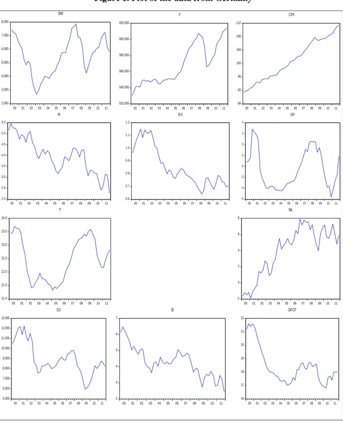
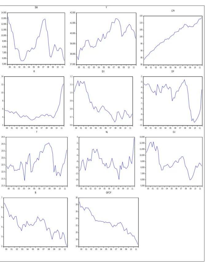
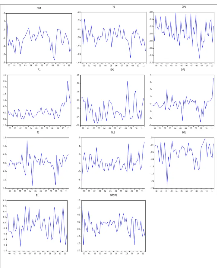
In order to analyse the behaviour of the financial and macroeconomic variables to be used in this study, we plot the graphs presented on the figures 1 and 2 and present the tables 2 and 3 with the descriptive statistic of these variables, which are in appendix. Observing the graphs on the figures
25
1 and 2, the stock market price indexes of the two countries present a similar behaviour except for the last two years of the observations in which the Germany stock market price index presents an increasing trend in opposite of Portugal stock market price index. However, according to the table 2 and 3 Portugal stock price index presents a mean higher than the stock price index from Germany.
Regarding the macroeconomic variables, observing the figures we noted that Germany always present a GDP higher than Portugal on the period observed. The average value for the GDP presented on the tables 2 and 3 confirm the prevalence of the Germany GDP over the GDP from Portugal. The consumer price index presents a similar behaviour for both countries. Concerning the debt of the Government and total economy, Portugal presents higher Government deficit and higher total economy net borrowing in percentage of GDP. By observing the figures 1 and 2, Germany presents a net lending to GDP for most of the years whereas Portugal always presents a negative net lending, as the maximum of the net lending to GDP ratio for the years observed is negative. In regards to the long term interest rate, the Germany interest rate presents a similar behaviour to US long term interest rate. As for Portugal’s interest rate, for the years observed, it presents always a higher interest rate than the Germany. Additionally, observing the tables 2 and 3, the maximum interest rate from Portugal is significantly higher than the maximum interest rate from Germany economy. Finally we observe that Portugal presents a higher ratio of gross fixed capital formation to GDP comparing to the ratio from Germany economy.
4.2 Methodology
Observing the graphs on the figures 1 and 2 presented on the appendix, we noted that these variables present some trend, positive or negative. This trend shows the possible presence of variables autocorrelation with their past value, and by observing these figures we can see that there
26
is no constant mean. So the variation of the mean over time and the autocorrelation with the past value show the presence of the unit root, which cause these variables to be non-stationary, one of the characteristics of the financial times series (Tsay 2005).
Using the non-stationary time series data in financial models may produce spurious and unreliable results. Therefore, the raw data that are non-stationary have to be transformed to the stationary data so as to allow a reliable result. So, in order to avoid the non-stationaryproblem, instead of working with the stock market price index and the level of the macroeconomic variables, we opted to work with the stock market return and the macroeconomic variables growth rate or changes that are variables, adopting a test for the unit root in time series, present to be stationary. Observing the figures 3 and 4 in appendix, we can see that the transformed variables, in opposite to the graphs on the figures 1 and 2, present no trend and vary around a constant mean, that is zero.
After presenting the transformed data to be used in this study, we present the equation model to study the effect of the macroeconomic variables changes on the stock market return.
SM1it = β0+β1Y1it + β2CPI1it + β3 R1it + β4 EX1it + β5 DF1it + β6 T1it + β7 NL1it + β8 DJ1it + β9 B1it + β10 GFCF1it +ɛit (2)
To make a robust conclusion about these time series stationary property, we adopted the Augmented Dickey-Fuller (ADF) test in order to test the unit-root of the transformed variables. The optimal lag length is determined based on the lowest value of the Schwarz criterion. The table 4 and 5 in appendix show the result of the stationary test for the variables employed in this study. The conclusion if a variable is or not stationary, is performed comparing the corresponding t-statistic on the table 4 and 5 with the critical values for the Dickey-Fuller unit root t-test t-statistic, presented on the figure 5 in appendix. According to the results presented on the table 4 and 5 for
27
the t-statistic, we conclude that the variables employed to test the effect of the economic activity level on the stock market return are stationary, according to the significant level specified on the tables.
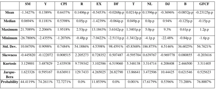
The descriptive statistics of the data employed for Germany and Portugal are presented on the tables 1 and 2 respectively, where the sample quarterly means, medians, maximums, minimums and standard deviations are presented, and so as the skewness, kurtosis, Jarque Bera and the p-value. The Germany stock return has a mean of 0.0019 per cent whereas Portugal stock return demonstrates a mean of -1.34 per cent. For the volatility of the stock markets return concerned, Germany stock market return presents a higher standard deviation comparing to Portugal, 10.51 per cent against 10.05 per cent. Regarding the macroeconomic variables, comparing the variables mean, Germany shows a mean for GDP growth rate equal to 0.3 per cent whereas the Portugal economy presents a mean for GDP growth rate of 0.14 per cent, Germany consumer price index average growth rate is lower than the average from Portugal, 0.42 per cent against 0.64 per cent. Regarding the difference between the average changes of government deficit and the economy net lending to GDP ratio of these two countries, Portugal presents a mean for the change of the government deficit to GDP ratio equal to -0.027p.p. while Germany presents a mean for the change of government deficit to GDP ratio equal to 0.018p.p., and Germany net lending to GDP ratio changes on average 0.15p.p. while Portugal net borrowing to GDP ratio changes on average 0.14p.p. Germany presents an interest rate that changes on average -0.067p.p. per quarter, while Portugal interest rate changes on average 0.14p.p. per quarter. Regarding the average change of the tax revenue to GDP ratio, the two economies do not display relevant difference. On the other side, the average change of Germany gross fixed capital formation to GDP ratio is higher than
28
Portugal ratio, Germany ratio changes on average -0.06p.p. while Portugal ratio changes on average -0.23p.p. per quarter.
The calculated skewness, kurtosis, Jarque Bera and the p-value are used to test the hypothesis that the data follow a normal distribution. To have a normal distribution, the skewness has to be equal to zero, the kurtosis equal to 3 and the p-value should be higher than 10 per cent. For Germany the normality is not reject for the growth of the consumer price index, exchange rate, and change of domestic interest rate, net lending to GDP ratio, foreign interest rate and the gross fixed capital formation to GDP ratio. For Portugal, the normality is not rejected for the stock return, the growth rate of GDP, consumer price index, exchange rate, and changes of the foreign interest rate, net borrowing and gross fixed capital formation to GDP ratio.
Table 1. Descriptive statistic of the data employed for Germany
SM Y CPI R EX DF T NL DJ B GFCF Mean 0.0019% 0.3038% 0.4238% -0.0673p.p -0.5456% 0.0177p.p -0.0113p.p 0.1542p.p -0.3696% -0.0852p.p -0.0604p.p Median 1.41% 0.3700% 0.4500% -0.095p.p -1.425% 0.0366p.p 0.03455p.p 0.4p.p 0.94% -0.125p.p -0.1p.p Maximum 23.84% 2.19% 1.06% 0.54p.p 13.18% 2.6204p.p 0.3242p.p 2.1p.p 9.3% 0.61p.p 0.8p.p Minimum -28.89% -4.1600% -0.65% -0.84p.p -7.04% -2.8902p.p -0.6392p.p -1.5p.p -22.48% -0.84p.p -1.p.p Std. Dev. 10.509% 0.9534% 0.3818% 29.7176% 4.5398% 78.71% 22.5708% 92.2983% 6.5146% 36.6025% 35.4148% Skewness -0.689067 -2.249087 -0.441846 -0.247493 0.727825 -0.239873 -0.909658 -0.077498 -0.969778 0.080855 0.310788 Kurtosis 3.653863 11.84063 2.828450 2.961603 3.100452 7.569517 3.557004 2.301859 4.208408 2.466500 3.583382 Jarque-bera 4.653578 196.7808 1.620685 0.492971 4.258011 42.22128 7.240324 1.022850 10.44425 0.621546 1.453382 Probability 9.7609% 0.0% 44.4706% 78.1543% 11.8956% 0.0% 2.6778% 59.9641% 0.5396% 73.288% 48.3506%
29
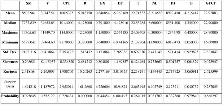
Table 2. Descriptive statistic of the data employed for Portugal
SM Y CPI R EX DF T NL DJ B GFCF Mean -1.3427% 0.1389% 0.6437% 0.1406p.p -0.5453% -0.0268p.p 0.0214p.p 0.1396p.p -0.3696% -0.0852p.p -0.23125p.p Median 0.0694% 0.1181% 0.5398% 0.05p.p -1.4239% -0.064p.p 0.049p.p 0.0p.p 0.94% -0.125p.p -0.15p.p Maximum 21.7089% 2.2066% 1.9518% 2.53p.p 13.1843% 3.6162p.p 1.3401p.p 5.0p.p 9.3% 0.61p.p 1.2p.p Minimum -26.7806% -2.4355% -1.2076% -0.48p.p -7.0422% -2.5131p.p -1.3412p.p -4.1p.p -22.48% -0.84p.p -1.6p.p Std. Dev. 10.0470% 0.9098% 0.7484% 54.1886% 4.5398% 98.4591% 45.8368% 186.875% 6.5146% 36.6025% 56.7621% Skewness -0.445820 -0.122072 0.008515 2.205273 0.728352 0.507487 -0.595704 0.639767 -0.969778 0.080855 -0.203616 Kurtosis 3.129001 3.487829 2.435938 9.739342 3.102586 6.519060 5.348138 3.314714 4.208408 2.466500 3.311405 Jarque-Bera 1.623326 0.595167 0.636911 129.7433 4.265025 26.82790 13.86641 3.472506 10.44425 0.621546 0.525623 Probability 44.4119% 74.2611% 72.7271% 0.0% 11.8539% 0.0% 0.001% 17.6179% 0.5396% 73.288% 76.8887%
After presenting the descriptive statistic of the data to be used to estimate the equation 2, we present the correlation between these data. The tables 6 and 7 in appendix show the correlation between the variables to be used in this study for the two counties.
By observing the table 6 in appendix, we perceive that the Germany stock return is correlated positively with all explanatory variables except with the growth of the exchange rate. Additionally, the variables that are more correlated with the Germany stock market return, with a correlation higher than 0.4 in absolute value, are the GDP growth rate, domestic and US long term interest rate changes, and the Dow Jones Industrial Average stock return.
Regarding the Portugal stock market return, observing the table 7 in appendix, it is positively correlated with GDP growth rate, Dow Jones Industrial return, and changes of US long term interest rate and gross fixed capital formation to GDP ratio. On the other side, we noted a negative relation between the Portugal stock market return and the growth rate of consumer price index, exchange rate, changes of the ratio of government deficit, tax revenue and net borrowing to GDP,
30
and domestic long term interest rate change. Moreover, the Portugal stock market return appears to be more correlated, with a correlation higher than 0.4 in absolute value, with the GDP growth rate, Dow Jones stock market return and US long term interest rate change.
Regarding the regression model, we opted to use the Ordinary Least Squared model. The least squared model assumes that the expected squared error value is equal at any point, so the regression estimated by the ordinary least square may be biased in the presence of conditional heteroskedasticity that occurs when we are working with data that have variances that have sudden increases or decreases and means variable over time. The conditional heteroskcedasticity is not common for low frequency data and, as we are working with quarterly data and by testing the possible presence of the heteroskedasticity, we conclude that all the variables used on the regression are homocedastic, there is no conditional heteroskedasticity. Observing the figures 6 and 7 in appendix, we may detect that the residual squared error are not correlated. We can observe that the p value is always higher than 10% for all the 20 lags considered, which deny the presence of the conditional heteroskcedasticity. Towards the absence of the conditional heteroskcedasticity, we adopt the OLS model so as to estimate the effect of the economic activity level on the stock market return.
31
5. Empirical results
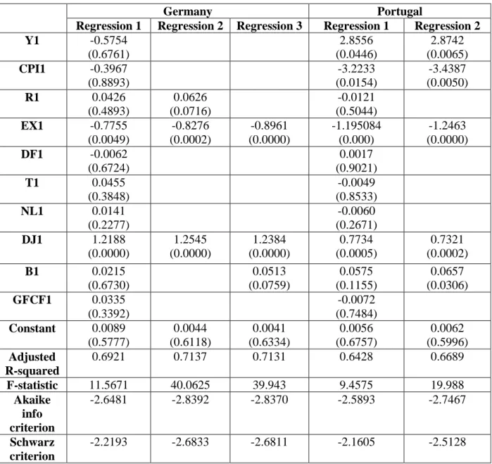
Applying the equation 2 and the regression model presented on the last section, we present the table 3 that contains the empirical results. Analysing the estimated coefficients on the regression 1 that considers all the explanatory variables, the Germany stock market return seems to be sensitive only for the exchange rate growth and the Dow Jones stock market return. For example, an increase of the rate, that the euro is exchange to dollar, by 1% would cause a depreciation of Germany stock market return by 0.77%, on the other side an increase of the Dow Jones stock return by 1% would change the Germany stock return by 1.22%. Regarding the Portugal stock market return, considering the regression 1 that also takes into account all the explanatory variables, this stock market return is sensitive, at 5% level, to the growth rate of GDP, consumer price index and exchange rate, Dow Jones stock return and to the US long term interest rate change. Observing the table below, we can observe that a change of 1% on the growth rate of GDP, consumer price index, exchange rate, Dow Jones return and a change of 1p.p of US long term interest rate cause a change on Portugal stock market return of 2.86%,-3.22%, -1.19%, 0.77% and 5.75% respectively.
Excluding the statistically non-significant variables for Germany stock return, we consider on the regression 2 and 3 only the growth of the exchange rate, the Dow Jones stock return and the domestic or foreign long term interest rate changes. As we can observe, neither the domestic or foreign long term interest rate changes were statistically significant on the first regression estimated. As the correlation between them is significant, we decided not to include both variables on the same regression which cause the variable not excluded to be statistically significant. As they are positively correlated, their effects on Germany stock return have the same sign. Considering the regression 2, if the domestic interest rate change by 1p.p the Germany stock return increase by 6.25%. On the other side, considering the regression 3, if the US long term interest
32
rate change by 1p.p the Germany stock return increase by 5.13%. Regarding to the Portugal stock market return regression, considering only the statistically significant variables on the regression 2, these variables effect similarly when considering all the explanatory variables. A change of 1% on the growth rate of GDP, consumer price index, exchange rate, Dow Jones stock return and a change of 1p.p of US long term interest rate cause a change on Portugal stock market return of 2.87%, -3.44%, -1.25%, 0.73% and 6.56% respectively.
Excluding the statistically non-significant variables on the regression 1 from Germany and Portugal, the adjusted R squared increases and the Akaike info and Schwarz criterion decrease, which show an improvement of the new estimated regressions.
In comparison, the results found when applying the study to Germany stock return are consistent with other stock market empirical results. Rufus (2007) found that the domestic interest rate affects positively the stock market price and the exchange rate affects negatively the Nigerian stock exchange, Chancharat et al (2007) and Hsing(2011) found that the domestic stock market price under their studies are positively influenced by the performance of the foreign stock market, Kuwornu (2011) found that the exchange rate affect negatively Ghana stock market return. However, the results for Germany stock return are different from Abdullah and Hayworth (1993) that found that the long-term interest rate has a negative effect on the stock return, Christopher et al (2006) that defend that the exchange rate doesn’t affect the New Zealand stock return.
Regarding the results found for Portugal stock market return, they are also consistent with others stock market empirical results. Humpe and Macmillan (2007) found that the US stock price is affected negatively by the consumer price index and long term interest rate, Hsing(2011) that defended that the GDP and the foreign financial market affect positively the domestic stock market price, and the consumer price index and long-term interest rate affect negatively the stock market
33
price. In opposite for the results found for Portugal stock return, we have Rufus (2007) and Kuwornu (2011) that found that the consumer price index affect positively the stock market price, Christopher et al (2006) that deny the significance of the inflation and exchange rate effect on the stock market price.
Table 3. Estimated regression for Germany and Portugal stock market return by OLS
Germany Portugal
Regression 1 Regression 2 Regression 3 Regression 1 Regression 2
Y1 -0.5754 (0.6761) 2.8556 (0.0446) 2.8742 (0.0065) CPI1 -0.3967 (0.8893) -3.2233 (0.0154) -3.4387 (0.0050) R1 0.0426 (0.4893) 0.0626 (0.0716) -0.0121 (0.5044) EX1 -0.7755 (0.0049) -0.8276 (0.0002) -0.8961 (0.0000) -1.195084 (0.000) -1.2463 (0.0000) DF1 -0.0062 (0.6724) 0.0017 (0.9021) T1 0.0455 (0.3848) -0.0049 (0.8533) NL1 0.0141 (0.2277) -0.0060 (0.2671) DJ1 1.2188 (0.0000) 1.2545 (0.0000) 1.2384 (0.0000) 0.7734 (0.0005) 0.7321 (0.0002) B1 0.0215 (0.6730) 0.0513 (0.0759) 0.0575 (0.1155) 0.0657 (0.0306) GFCF1 0.0335 (0.3392) -0.0072 (0.7484) Constant 0.0089 (0.5777) 0.0044 (0.6118) 0.0041 (0.6334) 0.0056 (0.6757) 0.0062 (0.5996) Adjusted R-squared 0.6921 0.7137 0.7131 0.6428 0.6689 F-statistic 11.5671 40.0625 39.943 9.4575 19.988 Akaike info criterion -2.6481 -2.8392 -2.8370 -2.5893 -2.7467 Schwarz criterion -2.2193 -2.6833 -2.6811 -2.1605 -2.5128
Note: The figures in the parenthesis are the p values. A p value higher than 10% reject the
34
6. Conclusion
In this study we have analysed the relation between the stock market price index and the key macroeconomic variables which reflect the economic activity level. The model and variables used to study the effect of the macroeconomic variables on the stock market price are similar to those used by the author Hsing on his studies from 2011. In addition to the variables used by the author, we extend the model by introducing the ratio of the economy net lending and gross fixed capital formation, to GDP.
The time series used in this study comprise quarterly observations from Germany and Portugal stock market price index, gross domestic product, consumer price index, domestic long term interest rate, exchange rate, Dow Jones Industrial Average price index, US long term interest rate and the ratio of public deficit, tax revenue, net lending and gross fixed capital formation, to GDP, from January of 2000(Q1) to December of 2011(Q4).
According to the results found by applying the OLS regression model, the Germany stock market return showed to respond only to domestic and foreign long term interest rate changes, the growth of the exchange rate and the Dow Jones Industrial return. In opposite to our assumptions previously presented, the domestic long term interest rate affects positively this stock return. This positive effect may be explained by the fact that the increase of the domestic interest rate tends to attract the capital inflow and the demand for stock, and in turn increase the stock price. The foreign interest rate change affects positively the Germany stock return. This positive effect may be explained by the fact that, the increase of the foreign interest rate depreciates the domestic currency and in turn increases the net export. In agreement to our assumptions, the Dow Jones return affects positively the Germany stock return, as the two stock market are positively highly correlated. The
35
exchange rate negatively affects the Germany stock return, as its depreciation increase the import cost and decrease the capital inflow.
Regarding the Portugal stock market return, in accordance to the assumptions previously presented, it is positively affected by the GDP growth rate and the Dow Jones Industrial return. The US long term interest rate change affects positively the Portugal stock return, this positive effect may be explained by the fact that a foreign interest rate increase tends to increase the net export by depreciating the exchange rate. The consumer price index growth, in accordance to our assumptions, negatively impacts the Portugal stock return. The exchange rate negatively affects the Portugal stock return, as the depreciation of the domestic currency tends to decrease the capital inflow and increase the import cost.
Concerning the regulatory authorities’ actions, there are several policy implications. To promote a robust stock market the authorities need to pursue the economic growth, appreciation of the exchange rate, and manage the interest rate and the inflation rate. The GDP growth contributes to the increase of the purchase power and the investment opportunities, and consequently to the increase of the corporate profit. In order to decrease the investment cost and to promote the capital inflow, and in succession the demand for stock, the regulatory entities should manage the interest rate and the inflation rate, as they are positively correlated, according to the effect of these variables on the stock market performance. The appreciation of the euro exchange rate would help to increase the capital inflow and reduce the import cost. The authorities should also monitor the external factor, such as the Dow Jones index and the US long term interest rate so as to forecast their impact on the domestic stock price when any changes occur.
36
One of this study limitations is, as the smallest period available for most of the macroeconomic variables is quarterly, the size of the sample used is not sufficiently large for the period considered. Additionally, given the fact that we are working with economic time series, there is some evidence of multicollinearity between the explanatory variables. The evidence of multicollinearity makes some variables that are significantly correlated with the dependent variable, to be statistically non significance when all the variables are taken into account.
Finally, there are some points that may provide grounds for further research. The addition of more variables that may help to better explain the variation of the stock prices and the extending of this study to other components of the financial market.
37
Bibliography references
Abdul, R., 2008, Macroeconomic variables and stock market performance: Testing for dynamic linkages with known structural break, Savings and Development, 32: 77-102.
Abdullah, D. and Hayworth, S., 1993, Macroeconometrics of stock price fluctuations, Quarterly
Journal of Business and Economics, 32: 50-67.
Adampoulos, A., 2012, Financial development and economic growth a comparative study between 15 European Union Member-States, International Research Journal of Finance and Econimics, 35: 143-149.
Agrawal, G., Srivatastav, A. and Srivastava, A., 2010, A study of exchange rates movement and stock market volatility, International Journal of Business and Management, 5: 62-73.
Alam, M. and Uddin, G., 2009, Relationship between interest rate and stock price: Empirical evidence from developed and developing countries, International Journal of Business
and Management, 4.
Arestis, P., Demetriades, P. and Luintel, K., 2001, Financial development and Economic Growth: The Role of Stock Markes, Journal of Money, Credit and Banking, 33: 16-41.
Asaolu, T.O. and Ogunmuyiwa, M.S., 2011, An econometric analysis of the impact of macroeconomic variables on stock market in Nigeria, Asian Journal of Business Management, 3: 72-78.
Bekhet, H. and Othman, N., 2012, Examining the role of fiscal policy in Malaysian stock market,
International Business Research, 5: 59-67.
Bollerslev, T., 1986, Generalized autoregressive conditional heteroskedasticity, Journal of
Econometrics, 31: 307-327.
Chancharat, S., Valadkhani, A. and Harvie, C., 2007, The influence of international stock markets and macroeconomic variables on the Thai stock market, Applied Econometrics and International
Development,7(1).
Christopher, G., Minsoo, L., Hua, Y. and Jun, Z., 2006, Macroeconomic variables and stock market interaction: New Zealand evidence, Investment Management and Financial Innovations, 3: 89-101.
Darrat, A., 1990, Stock returns, money and fiscal deficits, The Journal of Financial and
38
Demirguc-Kunt, A., Feyen, E. and Levine, R., 2011, Optimal financial structures and development: The evolving importance of banks and Markets.
Duca, G., 2007, The relationship between the stock market and the economy, Bank of Valletta
Review, 36.
Engle, R., 2011, The use of ARCH/GARCH models in applied econometrics, Journal of
Economics Perspectives, 15: 157-168.
Horobet, A., Dumitrescu, S. and Dumitrescu D., 2009, Uncovered interest parity and financial market volatility, The Romanian Economic Journal, 32: 21-45.
Hsing, Y., 2011a, The stock market and macroeconomic variables in a BRICS country and policy implications, International Journal of Economics and Financial Issues, 1: 12-18.
Hsing, Y., 2011b, Impacts of macroeconomic variables on the stock market Bulgaria and policy implications, East-West Journal of Economics and Business, 2: 41-53.
Hsing, Y., 2011c, Macroeconomic determinants of the stock market index and policy implications: the case of a central European country, Eurasian Journal of Economics and Business, 4: 1-11. Hsing, Y., 2011d, Effects of macroeconomic variables on the stock market: The case of Czech Republic, Theoretical and applied economics, 7: 53-64.
Hsing, Y., 2011e, Impacts of macroeconomic variables on the U.S. stock market index and policy implications, Economics Bulletin, 31: 883-892.
Humpe, A. and Machillan, P., 2007, Can macroeconomic variables explain long term stock market movements? A comparison of the US and Japan, Centre for dynamic macroeconomic analysis, 07/20.
Huybens, E. and Smith, B., 1999, Inflation, financial markets and long-run real activity, Journal
of Monetary Economics, 43: 283-315.
Kuwornu, J., 2011, Macroeconomic variables and stock market returns: full information maximum likelihood estimation, Research Journal of Finance and Accounting, 4.
Lane, P., and Milesi-Ferretti, G., 2003, International Financial Integration, IMF Third Annual
Research Conference, 50: 82-113.
Levine, R. and Zervos, S., 1998, Stock market, banks and economic growth, The American
Economic Review, 88: 537-558.
Moldovan, I. and Medrega, C., 2011, Correlation of international stock market before and during the subprime crisis, The Romanian Economic Journal, 40: 173-193.
39
Nai-Fu, C., Richard, R. and Stephen, A.R., 1986, Economics forces and the stock market, The
Journal of Business, 59: 383-403.
Oskooe, S., 2010, Emerging stock market performance and economic growth, American Journal
of Applied Sciences, 7(2): 265-269.
Rahman, L. and Uddin J., 2009, Dynamic relationship between stock prices and Exchange rates: Evidence from three South Asian countries, International Business Research, 2.
Ramin, M., Lee, H. and Mohamed, H., 2004, Relationship between macroeconomic variables and stock market indices: cointegration evidence from stock exchange of Singapore’s All-S sector indices, Journal Pengurusan, 24: 47-77.
Ray, S., 2012, Testing granger causal relationship between macroeconomics variables and stock price behaviour: evidence from India, Advances in Applied Economics and Finance,3: 2167-6348. Rufus, O., 2007, The relationship between stock prices and macroeconomic factors in the Nigerian stock market, African review of money finance and banking, 79-98.
Solnik, B., 1983, The relation between stock prices and inflationary expectations: The international evidence, The Journal of Finance, 1: 35-48.
Tsay, R., 2005, Analysis of Financial Time Series, 2nd Ed. University of Chicago: A John Willey &Sons, INC., Publication.
40
Appendix
Table 1. Data description and sources1
Variables Description Source
FM The stock exchange quarterly average price index. DATASTREAM Y Gross domestic product in millions of national currency, chained
in volume and seasonally adjusted.
OECD
CPI Harmonized consumer price index for all items, where 2005 is the base year.
OECD
R Domestic long term government bond yield. OECD
EX The nominal exchange rate. National units per US-Dollar. OECD DF Government deficit ratio to GDP. Government deficit is equal to
the difference between total revenue 2 and total expenditure3.
EUROSTAT
T Tax revenue ratio to GDP. Taxes composed by indirect, direct and capital taxes.
EUROSTAT
NL Net lending or borrowing of the total economy as percentage of GDP, seasonality adjusted and adjusted by working day.
EUROSTAT
DJ Dow Jones Industrials quarterly average price index. DATASTREAM
B US long term government bond yield. EUROSTAT
GFCF Gross fixed capital formation as percentage of GDP, seasonally adjusted and adjusted by working day.
EUROSTAT
____________________________________________
1As this study is applied to two different countries, instead of working with the government deficit, tax revenue,
economy net lending and gross fixed capital formation in millions of national currency, we opted to work with the ratio of these variables to GDP. The ratio to GDP allow us to have a clearer idea of the reality of the economy.
2Total revenue is composed by taxes, social contributions, sales, other current revenue and capital revenue.
3Total expenditure is composed by intermediate consumption, compensation of employees, interest, subsidies, social
benefits, other social benefits, other current expenditure, capital transfers payable, capital transfers payable, capital investments and gross fixed capital formation.
41
Figure 1. Plot of the data from Germany
520,000 540,000 560,000 580,000 600,000 620,000 00 01 02 03 04 05 06 07 08 09 10 11 Y 88 92 96 100 104 108 112 00 01 02 03 04 05 06 07 08 09 10 11 CPI 2.0 2.5 3.0 3.5 4.0 4.5 5.0 5.5 00 01 02 03 04 05 06 07 08 09 10 11 R 0.6 0.7 0.8 0.9 1.0 1.1 1.2 00 01 02 03 04 05 06 07 08 09 10 11 EX -5 -4 -3 -2 -1 0 1 2 00 01 02 03 04 05 06 07 08 09 10 11 DF 21.0 21.5 22.0 22.5 23.0 23.5 24.0 00 01 02 03 04 05 06 07 08 09 10 11 T -2 0 2 4 6 8 00 01 02 03 04 05 06 07 08 09 10 11 NL 5,000 6,000 7,000 8,000 9,000 10,000 11,000 12,000 13,000 00 01 02 03 04 05 06 07 08 09 10 11 DJ 2 3 4 5 6 7 00 01 02 03 04 05 06 07 08 09 10 11 B 16 17 18 19 20 21 22 00 01 02 03 04 05 06 07 08 09 10 11 GFCF 2,000 3,000 4,000 5,000 6,000 7,000 8,000 00 01 02 03 04 05 06 07 08 09 10 11 SM
42
Figure 2. Plot of the data from Portugal
37,000 38,000 39,000 40,000 41,000 42,000 00 01 02 03 04 05 06 07 08 09 10 11 Y 80 85 90 95 100 105 110 115 00 01 02 03 04 05 06 07 08 09 10 11 CPI 2 4 6 8 10 12 14 00 01 02 03 04 05 06 07 08 09 10 11 R 0.6 0.7 0.8 0.9 1.0 1.1 1.2 00 01 02 03 04 05 06 07 08 09 10 11 EX -11 -10 -9 -8 -7 -6 -5 -4 -3 -2 00 01 02 03 04 05 06 07 08 09 10 11 DF 21.0 21.5 22.0 22.5 23.0 23.5 24.0 24.5 00 01 02 03 04 05 06 07 08 09 10 11 T -16 -14 -12 -10 -8 -6 -4 -2 0 00 01 02 03 04 05 06 07 08 09 10 11 NL 5,000 6,000 7,000 8,000 9,000 10,000 11,000 12,000 13,000 00 01 02 03 04 05 06 07 08 09 10 11 DJ 2 3 4 5 6 7 00 01 02 03 04 05 06 07 08 09 10 11 B 16 18 20 22 24 26 28 30 00 01 02 03 04 05 06 07 08 09 10 11 GFCF 5,000 6,000 7,000 8,000 9,000 10,000 11,000 12,000 13,000 14,000 00 01 02 03 04 05 06 07 08 09 10 11 SM