Comparison of Methods for Determining Precompression Stress Based on Computational Simulation

(1)

* Corresponding author:

Received: June 24, 2015

Approved: July 25, 2015

How to cite: Silva AR, Lima RP. Comparison of Methods for Determining Precompression Stress Based on Computational Simulation. Rev Bras Cienc Solo. 2016;40:e0150164.

Copyright: This is an open-access article distributed under the terms of the Creative Commons Attribution License, which permits unrestricted use, distribution, and reproduction in any medium, provided that the original author and source are credited.

Comparison of Methods for

Determining Precompression Stress

Based on Computational Simulation

Anderson Rodrigo da Silva(1)_{and Renato Paiva de Lima}(2)*

(1)

Instituto Federal Goiano, Departamento de Agronomia, Urutai, Goiás, Brasil. (2)

Universidade de São Paulo, Departamento de Ciência do Solo, Piracicaba, São Paulo, Brasil.

ABSTRACT: There are many methods for determining precompression stress (σp), whose value is affected by the slope of the soil compression curve. This study was designed to evaluate the hypothesis that for a certain compression curve all methods used to determine σp present the same value and accuracy. The aim of this study was to compare the accuracy and the relationship among seven of these methods by computational simulation of soil compression curves under nine scenarios. The following methods were used: Casagrande, Pacheco Silva, intersection of the initial void ratio with the virgin compression line (VCLzero), and the regression methods based on 2 (reg1), 3 (reg2), 4 (reg3), and 5 (reg4) points for modeling the elastic curve. Under each scenario, created by combining the swelling and the compression indices, 1,000 compression curves were computationally simulated via the Monte Carlo method. Subsequently, 95 % percentile confidence intervals were built using the 1,000 estimates of σp from each method under each scenario. Most of the differences among the methods were detected under scenarios consisting of high swelling and low compression indices. In general, Casagrande, Pacheco Silva, and reg4 were strongly correlated and presented the highest values of σp, as well as similar variability. The latter two can be considered as alternatives to the standard method of Casagrande, except for Pacheco Silva when the curve has a low compression index (≤0.2) and from medium to high swelling index (≥0.025), for which differences (p<0.05) were detected.

(2)

INTRODUCTION

Soil compaction as an effect of agricultural machinery has been one of the great challenges of modern agriculture (Lima et al., 2015). Vast cultivated areas have received increasingly heavy and intensive machine traffic (Mosaddeghi et al., 2007; Lima et al., 2015), especially at crop harvest. This has adverse effects on crop production and the environment (O’Sullivan et al., 1999). According to Cavalieri et al. (2008), soil compaction has been a subject of study for many years due to its implications for crop yield.

Compaction can be understood by studying soil compressibility (Dias Júnior and Pierce, 1995). Compression is characterized by a mechanical process that describes the decrease in volume when soil is exposed to a mechanical load, which is defined by a soil compression curve. Three important parameters extracted from the soil compression curve were describe by Keller et al. (2011): the swelling or recompression index (Cs), the compressibility coefficient (Cc), and the preconsolidation or precompression stress (σp), where Cs is defined as the slope of the swelling line (SL) and Cc is the slope of the Virgin Compression Line (VCL).

The Cs is used as a measure of rebound and soil mechanical resilience, reflecting the first part of the curve subjected to historical stress, characterized by elastic deformation (recoverable). The second part is the VCL, for which plastic deformations are irreversible. This part can be verified by the Cc value, not subject stress (Keller et al., 2011). Finally, σp is mathematically defined as the point that divides the compression curve into the elastic and plastic parts of the soil compression curve (Casagrande, 1936).

There are many methods for determination of σp. The most widely used was proposed by Casagrande (1936), which is based on the maximum curvature point of the soil compression curve. Nevertheless, other methods have been developed, such as the Pacheco Silva (ABNT, 1990) method, based on the intersection of the VCL and the initial void ratio. Dias Júnior and Pierce (1995) showed the procedure for determination of σp by intersection of two linear regressions made for VCL and SL, which can have a different number of points considered for fitting VCL and SL (Cavalieri et al., 2008). Another method (VCLzero) consists of considering σp as the value on the x-axis defined by the intersection of the VCL with a horizontal line from the initial void ratio (Arvidsson and Keller, 2004).

The studies of Arvidsson and Keller (2004), Gregory et al. (2006), Cavalieri et al. (2008), Ajayi et al. (2013), and An et al. (2015) demonstrated there are variations in the methods used for determination of the σp and that the shape of curve is an important source of variation of indices (σp, Cs, Cc) extracted from the soil compression curve, showing that further studies are required. However, these studies have in common many soils, moisture contents, textures, and different conditions in soil physical properties, which makes it hard to define the parameters of the compression curve for a specific study and more accurate analysis. Under these conditions, simulations can help create scenarios for reproducing experimental data (Tagar et al., 2015), which formalize and analyze some error propagation methods for modeling; among them, the Monte Carlo method has general applicability and can be used in models with mathematical formulations (Ortiz et al., 2004). This procedure was used by Ortiz et al. (2004), and simulations based on other methods were used by Oliveira et al. (2013, 2014) for soil data in Brazil.

(3)

METHODS

Methods for determination and calculation of indices

Seven methods for determination of σp were used: Casagrande, Pacheco Silva, intersection of initial void ratio with VCL (VCLzero), and linear regression methods based on 2, 3, 4, and 5 points for modeling of the elastic curve (swelling line, SL). An illustration of the regression method based on 2 points can be seen in figure 1.

The virgin compression line (VCL) was estimated through linear regression considering the last three points of the compression curve. The compressibility coefficient (Cc) was estimated as the slope of the linear regression fitted for VCL, determined as shown in equation 1, where e is the void ratio. The swelling index (Cs) was determined as the mean slope of the loading path up to 25 kPa (Equation 2), according to Keller et al. (2011). The Cc and Cs indices are identified on the compression curve and graphically represented in figure 1.

C_c = – e1600 – e400

log₁₀ (1600) – log₁₀ (400) Eq. 1

C_s = – e25 – e0

log₁₀ (25) – log₁₀ (1) Eq. 2

Scenarios of simulation

We created scenarios based on the values of the swelling (recompression index) and compression indices (Keller et al., 2011). This allowed us to reproduce different compression curves, which are associated with the results of a soil compressibility test. Simulation was based on the result of a simple uniaxial compression test with loads of 1, 12.5, 25, 50, 100, 200, 400, 800, and 1,600 kPa. In this case, the loading of 1 kPa corresponds to the initial void ratio or bulk density, which was only to calculate the swelling line associated with the initial state of the soil sample (Keller et al., 2011; An et al., 2015).

Figure 1. Determination of precompression stress (σp) by reg1, regression method based on 2

points, expressed in terms of void ratio, as a function of the logarithm of applied stress (kPa); Virgin compression line (VCL); the slope of the VCL is denominated as the compressibility coefficient, Cc;

swelling index, Cs. Adapted from Keller et al. (2011).

Void ratio

Applied stress (kPa) 0.7

0.6

0.5

1 10 100 1.000

0.8 0.9

VCL

C_c C_s

σ_p

VC V L

C

C C_c

C_s

(4)

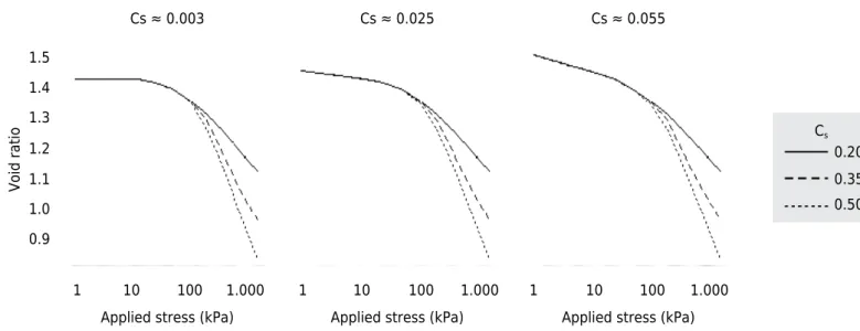
We combined three values of Cc and three values of Cs in order to create nine scenarios (Figure 2). The slopes of the VCL and SL were generated on the log10 scale of the applied loads. The original data set and the boundary of the initial void ratio and the values of Cc and Cs used in simulations were based on data from Ajayi et al. (2009), Keller et al. (2011), Ajayi et al. (2013), and An et al. (2015).

Simulation

Monte Carlo simulation was performed to compute mean and standard deviation. For each one of the nine compression curves described earlier, a fourth degree polynomial model was fitted, y = Xθ + ε, where y is the vector of void ratio, X is the polynomial model matrix, and ε is a random vector representing the error of the model. After that, we computed the vector of estimates (Equation 3) and its (co)variance matrix (Equation 4).

[

θˆ0

]

T

= ˆ

θ θˆ1 θˆ2 θˆ3 θˆ4

Eq. 3

Côv(θ) = (Xˆ T_X)–1_s2

Eq. 4

where s2

is the estimate of residual variance.

Subsequently, we considered the vector of estimates to be normally distributed as

N5 θ, Cov(θ)

[

ˆ ˆ

]

in order to simulate 1,000 other vectors of estimates, say ˆθ

*_{. For every}_θˆ i *

(i = 1, 2, ..., 1,000), a corresponding predicted vector ŷ_i= Xθˆ_i*_{was calculated. Finally,} the pairs (ŷi,x) were used to determine 1,000 random estimates of precompression stress, σ*

p, by each one of the seven methods.

Statistics for comparisons

We calculated the mean and coefficient of variation (%) of σ*

p determined by each method. In addition, a confidence interval was built using the percentile method, i.e., taking the quantiles σ_p*

(

)

2 α

and σp 1 ₂ * ₋α

)

(

as estimates of the lower and upper limits, respectively, of a 100(1 - α)% confidence interval.

Furthermore, we computed Pearson’s correlation matrix in order to study the relationship among the methods.

Figure 2. Simulation scenarios, created by combining three values of the compressibility coefficient (Cc) and three values of the

swelling index (Cs).

Cs 0.20

0.35 0.50

Applied stress (kPa) Applied stress (kPa) Applied stress (kPa)

Void ratio

Cs ≈ 0.003 Cs ≈ 0.025 Cs ≈ 0.055

1 10 100 1.000 1 10 100 1.000 1 10 100 1.000

(5)

Computing

All the simulations and data analyses were made using the software R 3.1.2 (R Core Team, 2015) soilphysics package (Silva and Lima, 2015). Calculation of σp was performed through the sigmaP() function. Simulations and percentile confidence intervals were performed using the simSigmaP() and plotCIsigmaP() functions, respectively.

RESULTS

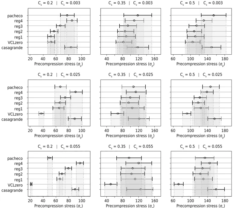
Considering scenarios where Cc = 0.2, the reg4 and Casagrande methods were similar and showed the highest values of σp for all the Cs conditions (Figure 3). The methods of Pacheco Silva, reg3, reg2, and reg1 changed more than Casagrande and reg4 with variation in Cs. The Pacheco method was similar to Casagrande when considering the smallest Cs, but they were statistically different (p<0.05) when Cs increased. The regression method had higher values when using more points for modeling the swelling line (reg4>reg3>reg2>reg1).

C_s ≈ 0.003 C_s ≈ 0.003 C_s ≈ 0.003

C_s ≈ 0.025 C_s ≈ 0.025

C_s ≈ 0.025

C_s ≈ 0.055 C_s ≈ 0.055 C_s ≈ 0.055

C_s = 0.2 C_s = 0.35 C_s = 0.5

C_s = 0.2

C_s = 0.35 C_s = 0.5

pacheco reg4 reg3 reg2 reg1 VCLzero casagrande

20 40 60 80 100 40 80 120 160 60 100 140 180

Precompression stress (σ_p)

Precompression stress (σ_p) Precompression stress (σ_p)

Figure 3. 95 % percentile confidence intervals for the mean of precompression stress (σp) determined by seven methods under nine

(6)

For Cc = 0.35, the Casagrande and reg4 methods also tended to show the highest values of σp. The VCLzero method showed the lowest values, regardless of Cs (Figure 3). The methods of Pacheco, reg3, reg2, and reg1 changed more than the Casagrande and reg4 methods with variation in Cs. As Cs increased, VCzero was the only method that was statistically different (p<0.05) than Casagrande.

For Cc = 0.50, the methods of Casagrande, Pacheco Silva, and reg4 showed the highest σp values. The VCLzero was statistically different (p<0.05) from Casagrande for all Cs. In general, the methods of Casagrande, Pacheco, and reg4 tended to show the largest values of σp. Specifically for Cc = 0.20, Casagrande and reg4 promoted the largest values, regardless of Cs. For Cc = 0.35 and 0.50, the general observation applies. The VCLzero method had the lowest values of σp for most scenarios. The Pacheco method was closer to Casagrande as Cs declined.

Under (Cc = 0.20, Cs ~ 0.055), we found the largest number of statistical differences (p<0.05) among the methods. In contrast, no difference (p>0.05) was found under the combination (Cc = 0.35, Cs ~ 0.003).

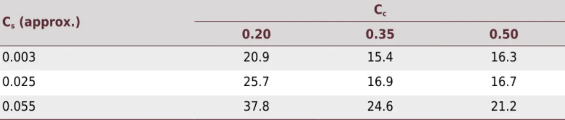
The variability shown by the methods in scenario (Cc = 0.20, Cs ~ 0.055) is noteworthy (Table 1). In fact, we observed ascending variability in the estimates according to the Cs, whatever the value of the Cc. Likewise, Cc = 0.20 tended to show the highest variability in the simulated means.

In all scenarios, the standard Casagrande method was more correlated (r>0.90) with the Pacheco method and regression method using 5 (reg4) and 4 (reg3) points (Table 2). Although VCLzero always tends to show the lowest value of σp, it had the same behavior as Pacheco and Casagrande. The reg1 and reg2 methods were related to each other in all scenarios.

DISCUSSION

Simulated soil compression curves

The curves simulated cover a wide range of soil compression curves, such as those obtained for soil samples in compression tests under different soil bulk densities, textures, and moisture contents (Arvidsson and Keller, 2004; Imhoff et al., 2004; Gregory et al., 2006; Cavalieri et al., 2008; Ajayi et al., 2009; Saffih-Hdadi et al., 2009; Ajayi et al., 2013; An et al., 2015).

A relationship between the simulated scenarios and situations of soil physical properties was observed. Ajayi et al. (2009) and Ajayi et al. (2013) obtained soil compression curves with lower values for Cc for samples with low water content. When water content increased, Cc also increased changing the shape of the soil compression curve.

For black and brown soils from Northeastern China under different bulk densities and water contents, An et al. (2015) obtained Cc values similar to those obtained by Ajayi et al. (2009) and Ajayi et al. (2013). They found that Cc was higher when water content in the

Table 1. Coefficient of variation for the simulated means of the seven methods in each scenario

defined by Cc and Cs

Cs (approx.)

Cc

0.20 0.35 0.50

0.003 20.9 15.4 16.3

0.025 25.7 16.9 16.7

(7)

soil samples increased. Variations in the shape of the curve when bulk density changed were also observed by Saffih-Hdadi et al. (2009) and An et al. (2015). They stated that Cc decreases for high bulk density values. According to the results obtained by An et al. (2015), the combination of high bulk density values and low water content minimizes the value of Cc.

The shape of the elastic line of a soil compression curve, represented here through Cs, varies mainly with water content, as observed by O’Sullivan and Robertson (1996) and Braida et al. (2008). However, the results found by O’Sullivan and Robertson (1996) show Cs values were higher in dry than in wet soils. However, Braida et al. (2008) found exactly the opposite, and attributed the results to the effects of the organic C and water content, which increasing the elastic proprieties of soil. Nonetheless, in any case, it is important to know that changing Cs increases the differences among the σp methods. This is most evident when comparing the methods under the same Cc value (Figure 3).

Behavior of the methods under each scenario

The slope of the elastic curve and VCL influenced the estimate of σp by the methods. Specifically, high values of Cs (0.055) and low values of Cc (0.2) increased differences among the methods (Figure 3). This can also be seen by the gradual increase in the

Table 2. Correlations among seven methods (C: Casagrande; V: VCLzero; r1, r2, r3, r4: regression methods; P: Pacheco Silva)

of determination of σp under nine scenarios designed according to the compression (Cc) and swelling (Ss) indices. Results based on 1,000 simulated soil compression curves

Cc = 0.2 | Cs = 0.003 Cc = 0.35 | Cs = 0.003 Cc = 0.5 | Cs = 0.003

V r1 r2 r3 r4 P V r1 r2 r3 r4 P V r1 r2 r3 r4 P

C 0.89 0.77 0.91 0.97 0.99 0.98 0.85 0.62 0.85 0.94 0.98 0.98 0.79 0.48 0.77 0.91 0.96 0.96

V - 0.70 0.81 0.85 0.87 0.96 - 0.52 0.71 0.79 0.81 0.95 - 0.36 0.58 0.68 0.72 0.93

r1 - - 0.97 0.91 0.85 0.78 - - 0.94 0.85 0.77 0.61 - - 0.93 0.80 0.69 0.46

r2 - - - 0.98 0.96 0.90 - - - 0.97 0.94 0.82 - - - 0.96 0.91 0.73

r3 - - - - 0.99 0.95 - - - - 0.99 0.92 - - - - 0.99 0.87

r4 - - - 0.97 - - - 0.95 - - - 0.91

Cc = 0.2 | Cs = 0.025 Cc = 0.35 | Cs = 0.025 Cc = 0.5 | Cs = 0.025

C 0.93 0.78 0.92 0.97 0.99 0.98 0.85 0.58 0.83 0.94 0.98 0.98 0.82 0.51 0.78 0.91 0.96 0.97

V - 0.78 0.88 0.91 0.92 0.98 - 0.49 0.69 0.78 0.81 0.94 - 0.40 0.61 0.71 0.75 0.93

r1 - - 0.97 0.91 0.86 0.83 - - 0.94 0.83 0.74 0.59 - - 0.94 0.81 0.72 0.51

r2 - - - 0.98 0.96 0.94 - - - 0.97 0.93 0.82 - - - 0.97 0.92 0.76

r3 - - - - 0.99 0.98 - - - - 0.99 0.92 - - - - 0.99 0.88

r4 - - - 0.98 - - - 0.95 - - - 0.93

Cc = 0.2 | Cs = 0.055 Cc = 0.35 | Cs = 0.055 Cc = 0.5 | Cs = 0.055

C 0.90 0.70 0.88 0.96 0.98 0.95 0.83 0.49 0.78 0.92 0.97 0.97 0.82 0.47 0.76 0.90 0.96 0.97

V - 0.66 0.79 0.85 0.86 0.96 - 0.43 0.65 0.75 0.78 0.93 - 0.42 0.63 0.73 0.76 0.93

r1 - - 0.96 0.88 0.81 0.82 - - 0.92 0.79 0.68 0.56 - - 0.93 0.80 0.69 0.52

r2 - - - 0.98 0.94 0.93 - - - 0.96 0.91 0.82 - - - 0.96 0.91 0.78

r3 - - - - 0.99 0.96 - - - - 0.99 0.92 - - - - 0.99 0.89

(8)

coefficient of variation (Table 1). When the variation among methods is analyzed under the same Cs, differences mainly occur under low Cc (Table 1). Variation among methods is largely influenced by the slope of VCL, Cc (Rosa et al., 2011).

Considering all scenarios, Casagrande, Pacheco Silva, reg4, and reg3 showed strong correlation (Table 2). Casagrande was compared with regression methods based on 2 (reg3) and 3 (reg4) points for modeling VCL (Arvidsson and Keller, 2004). These authors found that VCLzero was best correlated with Casagrande, but also found that the correlation between the regression method and Casagrande increased with the number of points (regression using three points>regression using two points), corroborating the results in table 2. However, Arvidsson and Keller (2004) did not test regression with four and five points (reg3 and reg4 as specified here, respectively), which would probably increase similarity with the Casagrande method, as found here. Cavalieri et al. (2008) showed medium to high correlations between regression methods and Casagrande (Cavalieri et al., 2008), at least higher than those obtained by Arvidsson and Keller (2004). The regression method using 4 and 5 points was correlated with Casagrande, as well as the Pacheco method (Table 2). Similarity between Casagrande and Pacheco in terms of σp also was found by Rosa et al. (2011).

Applicability of the methods

The Casagrande method has been considered as standard in almost all comparison studies involving soil compressibility. However, its algorithm is relatively complex, since the point of maximum curvature of the compression curve must be determined. Regression methods are considerably simpler since they consist of intercepting two regression lines. However, evaluations of the regression methods, including comparison of their performance with the Casagrande method, can be found in the studies of Dias Júnior and Pierce (1995), Arvidsson and Keller (2004), and Cavalieri et al. (2008).

CONCLUSIONS

Most of the differences among the methods were detected under scenarios consisting of high swelling and low compression indices.

In general, Casagrande, Pacheco Silva, and reg4 were strongly correlated, showing the largest values of σp, and similar variability. The latter two can be considered as alternatives to the standard Casagrande method, except for Pacheco Silva when the curve has a low compressibility coefficient (≤0.2) and medium to high swelling index (≥0.025), for which differences (p<0.05) were detected.

ACKNOWLEDGMENTS

We thank the Coordenação de Aperfeiçoamento de Pessoal de Nível Superior (CAPES, Brazil) for granting scholarships, and the Instituto Federal Goiano (Brazil) for financial support.

REFERENCES

Ajayi AE, Dias Júnior MS, Curi NC, Araújo Júnior CF, Souza TTT, Inda Júnior AV. Strength attributes and compaction susceptibility of Brazilian Latosols. Soil Till Res. 2009;105:122-7. doi:10.1016/j.still.2009.06.004

Ajayi AE, Dias Júnior MS, Curi NC, Oladipo I. Compressive response of some agricultural

soils influenced by the mineralogy and moisture. Inter Agrophys. 2013;27:239-46.

(9)

An J, Zhang Y, Yu N. Quantifying the effect of soil physical properties on the compressive

characteristics of two arable soils using uniaxial compression tests. Soil Till Res. 2015;145:216-23. doi:10.1016/j.still.2014.09.002

Arvidsson J, Keller T. Soil precompression stress. I. A survey of Swedish arable soils. Soil Till Res. 2004;77:85-95. doi:10.1016/j.still.2004.01.003

Associação Brasileira de Normas Técnicas - ABNT. NBR 12007: Ensaio de adensamento unidimensional. Rio de Janeiro: 1990.

Braida JA, Reichert JM, Reinert JM, Sequinatto LS. Elasticidade do solo em função da umidade e do teor de carbono orgânico. Rev Bras Cienc Solo. 2008;32:477-85. doi:10.1590/S0100-06832008000200002

Casagrande A. Determination of the pre-consolidation load and its practical significance. In:

Proceedings of the International Conference on Soil Mechanics and Foundation Engineering; 1936; Cambridge. Cambridge: Harvard University; 1936. p.60-4.

Cavalieri KMV, Arvidsson J, Silva AP, Keller T. Determination of precompression stress from uniaxial compression tests. Soil Till Res. 2008;98:17-26. doi:10.1016/j.still.2007.09.020

Dias Júnior MS, Pierce FJ. A simple procedure for estimating pre-consolidation pressure from soil compression curves. Soil Technol. 1995;8:139-51. doi:10.1016/0933-3630(95)00015-8

Gregory AS, Whalley WR, Watts CW, Bird NRA, Hallett PD, Whitmore AP. Calculation of the compression index and pre-compression stress from soil compression test data. Soil Till Res. 2006;89:45-57. doi:10.1016/j.still.2005.06.012

Imhoff S, Silva AP, Fallow D. Susceptibility to compaction, load support capacity, and soil

compressibility of Hapludox. Soil Sci Soc Am J. 2004;68:17-24. doi:10.2136/sssaj2004.1700

Keller T, Lamandé M, Schjønning P, Dexter AR. Analysis of soil compression

curves from uniaxial confined compression tests. Geoderma. 2011;163:13-23.

doi:10.1016/j.geoderma.2011.02.006

Lima RP, Rolim MM, Oliveira VS, Silva AR, Pedrosa EMR, Ferreira RLC. Load-bearing capacity and its relationships with the physical and mechanical attributes of cohesive soil. J Terramech. 2015;58:51-8. doi:10.1016/j.jterra.2015.01.001

Mosaddeghi MR, Koolen AJ, Hemmat A, Hajabbasi MA, Lerink P. Comparisons of different

procedures of pre-compaction stress determination on weakly structured soils. J Terramech. 2007;44:53-63. doi:10.1016/j.jterra.2006.01.008

Oliveira IR, Teixeira DB, Panosso AR, Camargo LA, Marques Júnior J, Pereira GT.

Modelagem Geoestatistica das incertezas da distribuição espacial do fósforo disponível no solo, em áreas de cana-de-açúcar. Rev Bras Cienc Solo. 2013;37:1481-91.

doi:10.1590/S0100-06832013000600005

Oliveira IR, Teixeira DB, Panosso AR, Marques Júnior J, Pereira GT. Modelagem e quantificação

da incerteza espacial do potássio disponível no solo por simulações estocásticas. Pesq Agropec

Bras. 2014;49:708-18. doi:10.1590/S0100-204X2014000900007

Ortiz JO, Felgueiras CA, Druck S, Monteiro AMV. Modelagem de fertilidade do solo por simulação estocástica com tratamento de incertezas. Pesq Agropec Bras. 2004;39:379-89.

doi:10.1590/S0100-204X2004000400012

O’Sullivan MF, Henshall JK, Dickson J. A simplified method for estimating soil compaction. Soil

Till Res. 1999;49:332-35. doi:10.1016/S0167-1987(98)00187-1

O’Sullivan MF, Robertson EAG. Critical state parameters from intact samples of two agricultural topsoils. Soil Till Res. 1996;39:161-73. doi:10.1016/S0167-1987(96)01068-9

R Core Team. R: A language and environment for statistical computing [internet]. Vienna, Austria: R Foundation for Statistical Computing; 2014 [accessed on: 17 Feb. 2014]. Available at: http://www.R-project.org/.

(10)

Saffih-Hdadi K, Défossez P, Richard G, Cui YJ, Tang AM, Chaplain VA. Method for predicting

soil susceptibility to the compaction of surface layers as a function of water content and bulk density. Soil Till Res. 2009;105:96-103. doi:10.1016/j.still.2009.05.012

Silva AR, Lima RP. Soilphysics: an R package to determine soil preconsolidation pressure. Comput Geosci. 2015;84:54-60. doi:10.1016/j.cageo.2015.08.008

Tagar AA, Changying J, Adamowski J, Malard J, Qi CS, Qishuo D, Abbasi NA. Finite element

simulation of soil failure patterns under soil bin and field testing conditions. Soil Till Res.