Submitted 15 July 2017 Accepted 30 March 2018 Published 8 June 2018 Corresponding author Inês Sousa, isousa@ualg.pt, inesgcsousa@gmail.com Academic editor Donald Kramer
Additional Information and Declarations can be found on page 19
DOI 10.7717/peerj.4653 Copyright
2018 Sousa et al. Distributed under
Creative Commons CC-BY 4.0
OPEN ACCESS
Soft-bottom fishes and spatial protection:
findings from a temperate marine
protected area
Inês Sousa1, Jorge M.S. Gon¸calves1, Joachim Claudet2,3, Rui Coelho1,4,
Emanuel J. Gon¸calves5and Karim Erzini1
1Centre of Marine Sciences—CCMAR, University of Algarve, Faro, Portugal
2National Center for Scientific Research, PSL Université Paris, CRIOBE, USR 3278 CNRS-EPHE-UPVD,
Maison des Océans, Paris, France
3Laboratoire d’Excellence CORAIL, France
4Instituto Português do Mar e da Atmosfera—IPMA, Olhão, Portugal
5MARE—Marine and Environmental Sciences Centre, ISPA—Instituto Universitário, Lisboa, Portugal
ABSTRACT
Numerous studies over the last decades have focused on marine protected areas (MPAs) and their effects on fish communities. However, there is a knowledge gap regarding how species that live associated with soft-substrates (e.g., sand, mud) respond to spatial protection. We analyzed abundance, biomass and total lengths of the soft-bottom fishes in a multiple-use MPA in the north-eastern Atlantic, the Luiz Saldanha Marine Park (Portugal), during and after the implementation of its management plan. Data were collected by experimental fishing in areas with three different levels of protection, during the implementation period and for three years after full implementation of the MPA. Univariate analysis detected significant biomass increases between the two periods. Fish assemblages were mainly structured by depth and substrate, followed by protection level. Community composition analyses revealed significant differences between protection levels and between the two periods. Species exhibited a broad variation in their response to protection, and we hypothesize that factors such as species habitat preferences, body size and late maturity might be underlying determinants. Overall, this study provides some evidence of protection effectiveness in soft-bottom fish communities, supported by the significant increase in biomass in the protected areas and the positive trends of some species.
SubjectsAquaculture, Fisheries and Fish Science, Conservation Biology, Ecology, Marine Biology, Natural Resource Management
Keywords Soft-bottom fishes, Marine protected areas, Reserve effect, Multivariate regression trees, Catch per unit effort
INTRODUCTION
The marine environment is nowadays increasingly impacted by human activities, with
overfishing reported worldwide (Myers & Worm, 2003;Pauly & Palomares, 2005). As a
consequence, conservation of marine fishes currently holds unique challenges for fisheries
managers (Vincent & Hall, 1996;Roberts, 1997). Marine protected areas (MPAs) are one
of the key tools to implement ecosystem-based management and marine spatial planning
uses, MPAs can promote the preservation and recovery of habitats and marine species, and are increasingly being used as tools for conservation and fisheries management (Roberts
& Polunin, 1993;Gaines et al., 2010). Through the reduction of fishing mortality, these
areas can enhance density, biomass, fish size and species diversity within their boundaries (Osenberg et al., 2011), which is often termed the ‘reserve effect’. Moreover, the transport of larvae (‘recruitment subsidy’) and movement of juveniles and adults (‘spillover’) to the
outside areas are expected to increase fisheries yields (Gell & Roberts, 2003;Grüss et al.,
2011).
MPAs include marine reserves or fully protected areas (FPAs), where extractive activities are prohibited (no-take zones), and partially protected areas (PPAs), which allow multiple uses (Lubchenco et al., 2003). PPAs offer a broad spectrum of protection levels, allowing either many human activities or just a few and like no-take zones, they have the potential
to enhance social and ecological benefits in coastal areas (Guidetti & Claudet, 2010;Claudet
& Guidetti, 2010;Sciberras et al., 2013;Sciberras et al., 2015;Horta e Costa et al., 2016).
For the achievement of conservation and management goals, it is important to understand the ecological effects of MPAs and the factors underlying these effects. The effectiveness of MPAs for the recovery of fish communities is affected by spatial
design (Halpern & Warner, 2002;Claudet et al., 2008), enforcement (Byers & Noonburg,
2007;Campbell et al., 2012;Bergseth, Russ & Cinner, 2015), habitat heterogeneity
(García-Charton & Pérez-Ruzafa, 1999), species movement ecology (Chapman et al., 2005;
Villegas-Ríos, Moland & Olsen, 2017) and life history traits (Jennings, Greenstreet & Reynolds, 1999;
Claudet et al., 2010;Hutchings et al., 2012). Life history traits, such as longevity, maximum
size, growth rate and reproductive potential, are important components of species responses to environmental stressors (e.g., temperature, toxicants, food availability) and fishing
exploitation (Jennings, Greenstreet & Reynolds, 1999;Denney, Jennings & Reynolds, 2002;
Hutchings et al., 2012;Audzijonyte & Kuparinen, 2016). Species habitat preferences and
inter-specific relations are acknowledged as important sources of complexity in spatial protection effectiveness, alongside with movement ecology (García-Charton &
Pérez-Ruzafa, 1999;Claudet et al., 2010). The fact that there is still no clear consensus on the
influence of migratory behavior as a determinant of protection effectiveness (Blyth-Skyrme
et al., 2006;Claudet et al., 2010) illustrates this complexity.
Despite the challenges posed by the study of spatial management, MPAs have been
shown to enhance the recovery and resilience of rocky (Claudet et al., 2006;Tetreault
& Ambrose, 2007;Sala et al., 2012) and coral reef fish (Russ & Alcala, 2004;Bruce et al.,
2012). However, there has been relatively little research on the response to protection of soft-bottom fish communities, probably because most MPAs target reef-associated species and because standard survey methods such as underwater visual census are regarded as not suitable for soft-bottom habitats, where fish densities are generally low (Giakoumi & Kokkoris, 2013).
Some MPA assessments have included multiple soft-bottom fish species among
extensive community studies (e.g., Dimech et al., 2008;Guidetti & Claudet, 2010), and
others addressed single soft-bottom species (e.g., Hunter et al., 2006;Wiegand, Hunter
reported that the ‘plaice box’, an area in the North Sea with seasonal fishing restrictions, favored the occurrence of larger fish. In the Western Atlantic, Georges Bank and southern New England fishing closures proved beneficial to several species of flounders and skates (Murawski et al., 2000), and significant increases in the abundance of winter flounder (Pseudopleuronectes americanus) and other fishes were reported after implementation of
a trawling closure on the Scotian Shelf (Fisher & Frank, 2002).Pipitone et al. (2000)also
described increases in the abundance and biomass of some soft-bottom fishes (e.g., Mullus
barbatusand Lepidotrigla cavillone) after a trawling ban in a Mediterranean MPA. More
recently,Donovan et al. (2016)reported the effects of a gillnet ban in a sandy coastal area
of Hawai‘i, and highlighted the variability of response according to species group, as only bonefishes (Albula spp.) exhibited a positive trend.
In this study we assessed the response to protection at the community and species level of the soft-bottom fish assemblage in the Luiz Saldanha Marine Park (LSMP), a coastal MPA in Portugal with predominantly soft-substrates (Henriques et al., 2014). Data were collected using standardized fishing procedures (trammel nets) inside and outside the marine reserve, over the implementation period and after the MPA was fully established. We used univariate and multivariate methods to analyze trends in community composition, fish abundance and biomass, and mean total length per species according to protection level, from before to after the full implementation of the MPA.
MATERIALS & METHODS
Study area
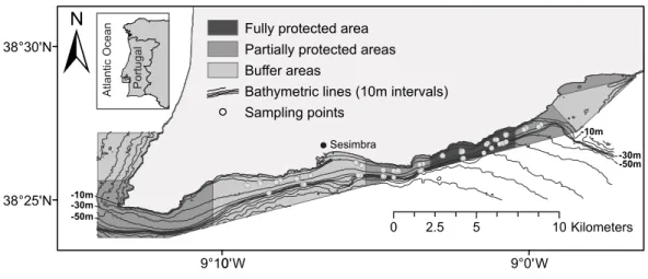
Located on the western coast of Portugal, the Luiz Saldanha Marine Park (LSMP) comprises 38 km of coastline characterized by high rocky cliffs alternating with sheltered bays. With
an area of 53 km2, the park includes many sublittoral habitat types, including hard and soft
substrates. Soft bottoms replace the coastal rocky reefs in most of the area at depths greater than 15–20 m. A substantial mud component is found in the sediment at depths greater than 30 m, while at shallower depths the dominant substrate is sand (medium, coarse and gravely sand) (Henriques et al., 2014). One interesting aspect to point out is the wide variety of soft-substrate habitats and benthic communities found in this area, as described by Henriques et al. (2014). The area has two nearby estuaries (Sado and Tejo) and is next to the Arrábida mountain chain, which shelters it from the dominant north winds. This region is also a biogeographic and oceanographic transition zone between warm and cold temperate
waters (Henriques, Gon¸calves & Almada, 1999;Lima et al., 2007) which, along with the
variety of available habitats (Henriques et al., 2014), makes it an important biodiversity
hotspot (Henriques, Gon¸calves & Almada, 1999;Gon¸calves, Henriques & Almada, 2002).
The MPA was created in 1998 as part of the Arrábida Natural Park, but it was only in August 2005 that the management plan started to be implemented. The management regulation main goals are to enhance the conservation of marine species and promote sustainable fisheries management (Gon¸calves, Henriques & Almada, 2002). Given the diversity of human activities, including recreational fishing, scuba diving and commercial fisheries, and the presence of two important fishing harbours: the port of Sesimbra, located
! ( ! ( ! ( ! ( ! (!(!(!( ! ( ! ( ! ( ! ( ! (!(!( ! (!(!( ! ( ! ( ! ( ! (!( ! ( ! ( ! ( ! (!( ! (!( ! (!( ! ( ! ( ! ( ! ( ! ( ! ( ! ( ! ( ! ( ! ( ! ( ! ( !( ! ( ! ( ! ( ! ( ! ( ! ( ! ( ! ( ! ( ! ( ! ( ! (!( ! ( ! ( ! ( ! (!( ! ( ! ( ! (!( ! ( ! ( ! (!( ! ( ! ( ! ( ! ( ! ( ! ( ! ( ! (!( ! ( ! ( ! ( ! ( ! ( ! ( ! ( ! ( ! ( ! ( ! ( ! ( ! ( ! ( ! ( ! ( ! ( ! ( ! ( ! ( ! (!( ! ( ! ( 9°0'W 38°30'N 38°25'N
±
0 2.5 5 10 Kilometers Portugal Atlantic Ocean Sesimbra -50m -30m -10m -50m -30m -10m (Fully protected area Partially protected areas Buffer areas
Bathymetric lines (10m intervals) Sampling points
9°100'W
Figure 1 Map of the Luiz Saldanha Marine Park (LSMP) zoning. The light grey dots indicate sampling points (experimental fishing).
Full-size DOI: 10.7717/peerj.4653/fig-1
within the MPA area, and the nearby port of Setúbal, spatial management was crucial. To mitigate conflicts related to multiple stakeholders and their divergent concerns (Vasconcelos et al., 2013), the LSMP regulations were established gradually over a four-year period and full implementation was achieved in August 2009 (implementation: 23rd Aug. 2005–23rd Aug. 2009; Year 1: LSMP area under buffer area protection level; Year 2: two PPAs were implemented; Year 3: two more PPAs were created, sampling started; Year 4: half of the FPA implemented; 23rd Aug. 2009—the FPA is fully implemented). The regulations
define different zones and levels of usage (Fig. 1). Trawling, dredging, purse seining and
spearfishing are prohibited in the entire area, and only licensed commercial vessels less
than 7 m long are allowed. The fully protected area (FPA) (4 km2) excludes all human
activities, with the exception of research and monitoring. The four partially protected areas
(PPA), totalling 21 km2, allow some recreational activities, including recreational diving,
and commercial fishing for cephalopods with octopus traps and jigs, although fishing is not allowed at distances less than 200 m from the shore. The three buffer areas (BA), totalling
28 km2, have the lowest level of protection. In addition to octopus traps and jigs (here
permitted close to the shore), longlines, trammel nets, gill nets and recreational fishing are allowed (nets at a distance beyond 463 m from the shoreline).
Data collection
Data were collected between November 2007 and May 2012 over a five years period: the first two years during the management plan implementation (period 1—implementation period: August 2007–August 2009) and three years after the MPA was fully implemented (period 2—after MPA full implementation: August 2009–August 2012). Sampling of the three protection levels occurred seasonally, each spring and autumn. Ten sampling
campaigns (experimental fishing) and 183 trammel net sets were undertaken (Fig. 1) (total
with the fishing procedure). Sampling area covered the FPA (n = 63), two adjacent PPAs (n = 61) and the larger BA (n = 59). To avoid spatial heterogeneity, areas in the eastern and western edges of the MPA were not included (west: proximity to cape; east: proximity to nearby estuary). Four sampling campaigns were undertaken during period 1 (n = 57) and six during period 2 (n = 126) (first three campaigns—four days each, 36 samples; following campaigns—seven days each, total of 147 samples; three samples per day). Two substrate types were sampled: sandy bottom, at 10–20 m (n = 112), and muddy bottom, at 30–45 m (n = 71) (samples: sand-BA: 36, PPA: 38, FPA: 38; mud-BA: 23, PPA: 23, FPA: 25). The BA was considered as the control in the spatial analysis of protection effect due to the allowed use of small-scale fishing gear: gill nets, trammel nets, longlines, jigs, pots and traps. The area surrounding the MPA was not chosen as a control because of greater depths and differences in bottom type. Each sample consisted of the catch of one monofilament trammel net (500 m long; 1.6 m high; inner panel stretched mesh of 100 mm; outer panel stretched mesh of 600 mm; soak time 22–24 h). Nets were set after sunrise and hauled about 24 h later. Each fish was identified on board to the species level and total length (TL) was measured to the nearest millimetre. Specimens were released afterwards, following ‘catch and release’ practice (The Portuguese Institute for Nature Conservation and Forests—ICNF approved the field surveys for this study; ICNF reference
no 00540 140307). Biomass was estimated using published length-weight relations (Table
S1—list of species with length-weight references, environment, maximum size and fisheries
category). Catch in number per unit effort (CPUE) and biomass per unit effort (BPUE) were calculated considering the unit effort as 500 m of trammel net and a soak time of 24 h. This provided average values (abundance and biomass) per sample that enabled comparisons of the three protection levels over time.
Data analysis
CPUE expressed as number of fish per 500 m of net (n·500 m−1) was considered as an
index of relative abundance and used along with biomass (BPUE—kg·500 m−1) to evaluate
differences between protection levels and trends over time (before and after full MPA implementation). Prior to data analysis, pelagic species (Auxis rochei, Boops boops, Sarda
sarda, Sardina pilchardus, Scomber spp., Trachurus spp.) were excluded from the dataset. Pelagic species are expected to be less meaningful in habitat characterization (Fréon & Misund, 1999) and therefore were not analyzed.
We used generalized linear mixed models (GLMM) (Breslow & Clayton, 1993) to test significance of protection level (BA, PPA, FPA), substrate (sand, mud) and period (period 1, period 2) as predictors of abundance and biomass. The interaction of protection level and substrate was included in the models to assess whether the effect of protection level was different in each substrate type. Sampling campaign (n = 10) was included as random variable to deal with correlation between observations and with the variability related with campaigns (Zuur et al., 2009). Models were fitted by maximum likelihood with Laplace approximation. Poisson and Gamma distributions (log link) were used to fit, respectively, abundance (discrete) and biomass (continuous) data. Variable selection was carried out by
likelihood ratio tests between nested models and by looking to the deviance explained by each variable, while model validation was carried out with visual inspection of the residuals (Zuur et al., 2009).
To analyse species spatial and temporal patterns, ratios of abundance, biomass and total length per species (for stingrays—Myliobatis aquila—dimension used was disc width) were also estimated and applied in accordance with a Before-After-Control-Impact (BACI)
analysis approach (Underwood, 1992;Underwood, 1994). Comparisons were made between
the buffer area (BA) and the two higher protection levels combined (PPA and FPA: PA—protected area), and between period 1 (implementation period) and period 2 (after full implementation) (protection level ratios included data from both periods; period ratios included data from the three protection levels). This specific analysis was done
for the species with frequency of occurrence higher than 15% (Table S2). The average
ratios (abundance, biomass and total length), standard errors (SE) and 95% confidence intervals (CI) were obtained by bootstrapping (9,999 permutations). The 95% confidence intervals were calculated using the adjusted bootstrap percentile method and used to check for significance (Payton, Greenstone & Schenker, 2003). To avoid problems resulting from small sample size, bootstrapping of total length was only performed for species with more than ten individuals per treatment (protection level or period). Hence, for total length comparisons, the species Citharus linguatula, Raja undulata and Solea solea were excluded from the protection level ratios, and C. linguatula, R. undulata and Rostroraja alba were excluded from the period ratios.
Multivariate procedures were applied to examine differences in fish assemblage according to protection level (PL) and time (period and year). The Hellinger transformation was used for abundance and biomass in order to overcome the problem of zero inflation (Legendre & Gallagher, 2001). Permutational multivariate analysis of variance (PERMANOVA) (Anderson, 2001) was performed to test significance of protection level, period and year as factors for community differences. Each constraint factor was assessed individually and then under interaction models: ‘protection level × period’ and ‘protection level × year’. Pairwise analyses were also obtained by comparing the protection levels within each period and comparing periods of each protection level.
The Euclidean distance matrix of transformed abundances was used in a principal components analysis (PCA). This technique provides visualization of multivariate data structure. It was used to explore the similarity between samples according to protection level and period. In order to compare samples, centroids per protection level and period, and dispersion ordiellipses (95% confidence interval) according to the weighted average scores of each protection level, were plotted. A second graphical output was also obtained with the species vectors in order to assess species contributions for community differences. Given the similarity of results obtained for abundance and biomass, the multivariate visualizations based on biomass are not presented.
To explore the main factors structuring fish assemblages, multivariate regression tree (MRT) analysis (De’Ath, 2002) was carried out using the Hellinger transformed abundances. The factors ‘protection level’ and ‘period’, and two environmental variables—depth and temperature were included. Substrate type was not included because it is correlated
with depth, and priority was given to the variable that incorporated more information (depth). This analysis creates clusters of sites by splitting the data according to explanatory variable threshold values and site similarity. The clusters and their dependence on the environmental data are represented graphically by a tree. Through this procedure, each cluster defines a species assemblage, and its environment type is described by the associated environmental values. MRT was performed given its ability to deal with discrete variables (in our case, protection level and period), non-linearity, and higher-order interactions among explanatory variables (De’Ath, 2002). The criterion for final model selection was minimization of cross-validated relative error (CVRE).
Indicator values (IndVal) (Dufrêne & Legendre, 1997) were calculated for each species in each node and terminal node (leaf). With this index, species are considered as indicators of a certain cluster of sites according to their relative abundance and relative frequency of occurrence within that group. Specifically, the product of relative abundance and relative frequency of occurrence of the species within a group is calculated and then multiplied by 100. The index takes the value of zero if there is no occurrences of the species within a group, increasing to 100 if the species occurs at all sites within a group and does not occur in any other group. A minimum of 10% contribution to the explained variance was required for a species to be considered as discriminant at a particular node and permutations were used to test for significance. Permutations were also used to assign significant discriminant species for each terminal node. A species was considered an indicator of a certain assemblage according to the cluster for which it had the highest IndVal.
All analyses were done using the R statistical software version 2.15.2 (R Core Team, 2014). The package vegan (Oksanen et al., 2014) was used for the multivariate analysis and the MRT was built with the package mvpart (Therneau & Atkinson, 2012).
RESULTS
In total, 8,820 fish of 70 species were recorded in the trammel net catches, of which 7,533 fish of 62 species were included in the analyses (eight pelagic species not included). The bony fishes were represented by 49 species and the elasmobranchs by 13 species. The list
of species and their frequency of occurrence is shown inTable S2. Overall, the local
soft-bottom fish community was dominated by three families of benthic fish, namely Soleidae (Solea and Pegusa), Triglidae (Chelidonichthys and Trigloporus) and Bothidae (Bothus and
Arnoglossus). Soleidae was the most abundant family (42%), followed by Triglidae (22%) and Bothidae (7%). In relation to biomass, Soleidae was still the dominant family (30%), although Rajidae was the second most important (28%), followed by Triglidae (12%).
Details of average abundance, biomass and total length per species are shown inTables S3
andS4.
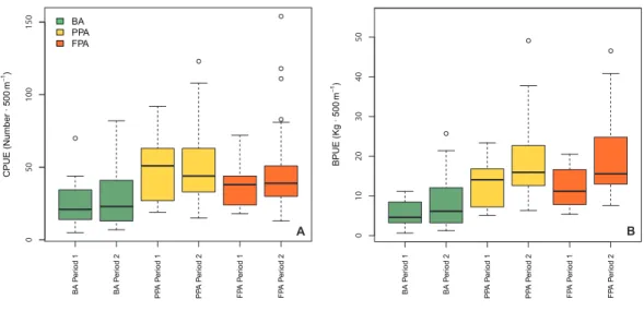
GLMM outputs (Table 1) revealed protection level and period as significant variables
in the biomass model (protection level: p< 0.001; period: p = 0.03), while protection level
and substrate were the significant variables in the abundance model (protection level:
p< 0.001; substrate: p < 0.001). These results are supported by the boxplots shown in
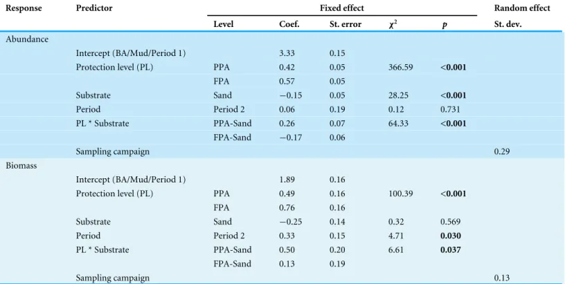
Table 1 Generalized linear mixed models of fish abundance and biomass. Results of the general linear mixed models (GLMMs) of fish abun-dance (CPUE n·500 m−1) and biomass (BPUE kg·500 m−1) according to protection level, period and substrate. The interaction ‘protection level ×
substrate’ was included and sampling campaign (n = 10) was considered as a random variable. GLMM of abundance and biomass used respectively, Poisson and Gamma distributions (log link).
Response Predictor Fixed effect Random effect
Level Coef. St. error χ2 p St. dev.
;Abundance
; Intercept (BA/Mud/Period 1) 3.33 0.15
; Protection level (PL) PPA 0.42 0.05 366.59 <0.001
; FPA 0.57 0.05 ; Substrate Sand −0.15 0.05 28.25 <0.001 ; Period Period 2 0.06 0.19 0.12 0.731 ; PL * Substrate PPA-Sand 0.26 0.07 64.33 <0.001 ; FPA-Sand −0.17 0.06 ; Sampling campaign 0.29 ;Biomass ; Intercept (BA/Mud/Period 1) 1.89 0.16
; Protection level (PL) PPA 0.49 0.16 100.39 <0.001
; FPA 0.76 0.16 ; Substrate Sand −0.25 0.14 0.32 0.569 ; Period Period 2 0.33 0.15 4.71 0.030 ; PL * Substrate PPA-Sand 0.50 0.20 6.61 0.037 ; FPA-Sand 0.13 0.19 ; Sampling campaign 0.13
FPA than in the BA, and that increases between period 1—period 2 are only apparent in biomass. The interaction of protection level and substrate was significant in both models
(abundance: p< 0.001; biomass: p = 0.037), indicating a different effect of protection level
according to substrate type. The coefficients indicate that mud had higher average values than sand (abundance, coef. sand = −0.15; biomass, coef. sand = −0.25), and that the sandy PPA had higher abundances in comparison to the sandy FPA (coef. FPA sand =
−0.17) (Fig. S1). This pattern is different in the muddy substrate, with higher values in
the FPA. Plots of abundance and biomass per protection level and substrate are shown in Fig. S1.
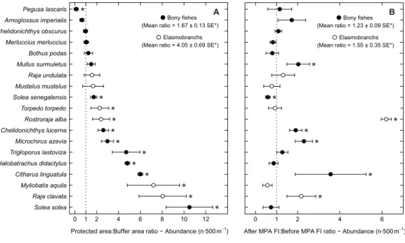
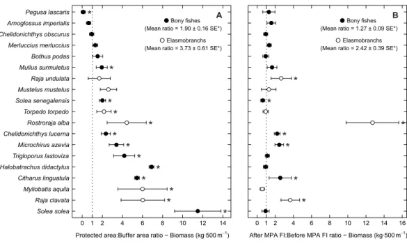
Examining abundance and biomass ratios between the BA and higher protection levels (Figs. 3and4), four flatfishes (Solea senegalensis, S. solea, C. linguatula, Microchirus azevia), four elasmobranchs (Torpedo torpedo, M. aquila, R. alba, Raja clavata), two gurnards (Chelidonichthys lastoviza and Chelidonichthys lucerna), and the Lusitanian toadfish (Halobatrachus didactylus) were found to be significantly more abundant in the PPA and FPA. Of these, R. clavata and S. solea were the ones with the greatest differences. All of these species also had significantly higher biomasses in the PPA and FPA. Regarding biomass, one more species, Mullus surmuletus, had higher values in the PPA and FPA.
Of the eleven species with higher abundance in the higher protection levels, five also had significant increases in abundance and biomass from period 1 to period 2, namely
01 02 03 04 05 0 BPUE (Kg ∙ 500 m −1) B 05 0 100 150 BA PPA FPA CPUE (Number ∙ 500 m −1) A BA Pe riod 1 BA Pe riod 2 PP A Pe riod 1 PP A Pe riod 2 FP A Pe riod 1 FP A Pe riod 2 BA Pe riod 1 BA Pe riod 2 PP A Pe riod 1 PP A Pe riod 2 FP A Pe riod 1 FP A Pe riod 2
Figure 2 Boxplots of fish abundance and biomass. Boxplots of fish abundance (A, CPUE—n·500 m−1)
and biomass (B, BPUE—kg·500 m−1) according to protection level (BA, buffer area; PPA, partially
pro-tected area; FPA, fully propro-tected area) and period (Period 1, Before MPA Full Implementation; Period 2, After MPA Full Implementation) (Box extent, 25th to 75th percentile; Band near the middle of the box, 50th percentile/median; Whiskers range, lowest to highest datum within the 1.5 × inter-quartile range in-terval).
Full-size DOI: 10.7717/peerj.4653/fig-2
C. linguatula, R. alba, R. clavata, C. lucerna and M. azevia. (Figs. 3and4). Other species showing positive changes over time were M. surmuletus, which showed an increase in abundance, and R. undulata, which had higher biomass in period 2. Other interesting results were the higher numbers of Pegusa lascaris in the BA. Arnoglossus imperialis showed a non-significantly higher abundance in the BA. Regarding time trends, the sole S. senegalensis exhibited a significant decrease in both abundance and biomass.
Some species with positive trends in abundance and biomass also increased in average
total length, including R. alba, R. clavata, C. lucerna and M. azevia (Fig. 5). Other species,
with no significant trends of abundance or biomass, also showed an increase in average size, specifically Merluccius merluccius, Bothus podas, Mustelus mustelus and S. solea.
S. senegalensis, which decreased significantly in abundance, was another species with larger average sizes in the PA and in period 2. Conversely, both A. imperialis and Chelidonichthys
obscurusexhibited a decrease in average size from the first to the second period.
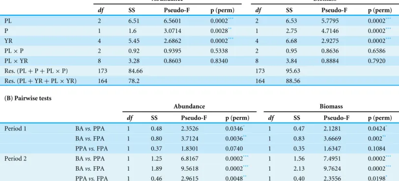
PERMANOVA on fish abundance and biomass (Table 2) revealed significant differences
for protection level (PL) and temporal factors (period and year). The effect of protection was not demonstrated by the interactions: the terms ‘PL × period’ and ‘PL × year’ were non-significant. However, pairwise comparisons detected some differences. Specifically, the FPA became significantly different from the PPA only in period 2, and when comparing within protection level, both the PPA and FPA communities showed significant differences between periods.
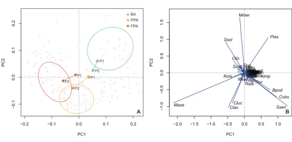
The PCA ordination confirmed the results of the protection level comparison (Fig. 6A),
with the BA centroids constituting a distinct group, and the PPA and FPA showing some overlap. The first axis explained 23.9% of the variation, with 34.9% of the variation
Protected area:Buffer area ratio − Abundance (n∙500m−1) Solea solea Raja clavata Myliobatis aquila Citharus linguatula Halobatrachus didactylus Trigloporus lastoviza Microchirus azevia Chelidonichthys lucerna Rostroraja alba Torpedo torpedo Solea senegalensis Mustelus mustelus Raja undulata Mullus surmuletus Bothus podas Merluccius merluccius Chelidonichthys obscurus Arnoglossus imperialis Pegusa lascaris 0 1 2 4 6 8 10 12 Bony fishes (Mean ratio = 1.67 ± 0.13 SE*)
Elasmobranchs (Mean ratio = 4.05 ± 0.69 SE*)
* * * * * * * * * * * *
After MPA FI:Before MPA FI ratio − Abundance (n∙500m−1)
0 1 2 4 6 Bony fishes (Mean ratio = 1.23 ± 0.09 SE*)
Elasmobranchs (Mean ratio = 1.55 ± 0.35 SE*)
* * * * * * * A B
Figure 3 Abundance response ratio per species. Response ratios (±standard error: SE) of abundance per species for (A) Control-Impact (Protected area:Buffer area) and (B) Before-After (After MPA Full Im-plementation:Before MPA Full Implementation) comparisons (Protected area, fully protected area and partially protected area; Before MPA Full Implementation, Period 1; After MPA Full Implementation, Pe-riod 2; FI, Full Implementation). Protection level ratios included data from both pePe-riods and pePe-riod ra-tios included data from the three protection levels. Rara-tios> 1 indicate positive responses and significant ratios (according to 95% confidence interval) are marked with ‘*’. Species ordered according to increas-ing Control-Impact abundance response ratio. Bony fish species are marked with ‘•’ and elasmobranch species are marked with ‘◦’.
Full-size DOI: 10.7717/peerj.4653/fig-3
explained cumulatively with the inclusion of the second axis. This analysis provides information on inter-period variation and a progression along the first axis is evident for the PPA and FPA. In both these areas, period 1 is closer to the BA group. Species vectors are
shown in the second biplot (Fig. 6B). M. azevia (Maze), the most abundant species in our
dataset, was highly related to the first component (PC1), while M. merluccius (Mmer) was the most correlated with the second component (PC2). Both M. azevia and M. merluccius were more abundant in the muddy substrate, and this was also the case for S. solea (Ssol) and C. linguatula (Clin). The latter two species exhibited higher abundances in the FPA, along with R. clavata (Rcla). P. lascaris (Plas), which has its vector isolated in the top-right of the plot, was more abundant in the BA and over sandy bottoms. Another species with affinity with sand was S. senegalensis, shown in the bottom-right. It was found in higher
numbers in the PPA (Table S3—species abundance and biomass per protection level;
Table S5—species abundance per substrate).
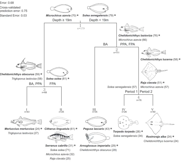
A multivariate regression tree (MRT) with four nodes and five leaves (terminal nodes)
was considered the most parsimonious to represent community structure (Fig. 7). This
model explained 32.2% of the species abundance variation and had an accuracy of 29% in assemblage association predictions. The primary split in the tree explained 19.6% of the species variation and separated fish assemblages according to depth, specifically depths less
Protected area:Buffer area ratio − Biomass (kg∙500 m−1) Solea solea Raja clavata Myliobatis aquila Citharus linguatula Halobatrachus didactylus Trigloporus lastoviza Microchirus azevia Chelidonichthys lucerna Rostroraja alba Torpedo torpedo Solea senegalensis Mustelus mustelus Raja undulata Mullus surmuletus Bothus podas Merluccius merluccius Chelidonichthys obscurus Arnoglossus imperialis Pegusa lascaris 0 1 2 4 6 8 10 12 14 Bony fishes (Mean ratio = 1.90 ± 0.16 SE*)
Elasmobranchs (Mean ratio = 3.73 ± 0.61 SE*)
After MPA FI:Before MPA FI ratio − Biomass (kg∙500 m−1)
0 1 2 4 6 8 10 12 14 16 Bony fishes (Mean ratio = 1.27 ± 0.09 SE*)
Elasmobranchs (Mean ratio = 2.42 ± 0.39 SE*)
* * * * * * * * * * * * * * * * * * * * A B
Figure 4 Biomass response ratio per species. Response ratios (±standard error: SE) of biomass per species for (A) Control-Impact (Protected area:Buffer area) and (B) Before-After (After MPA Full Imple-mentation:Before MPA Full Implementation) comparisons (Protected area, fully protected area and par-tially protected area; Before MPA Full Implementation, Period 1; After MPA Full Implementation, Pe-riod 2; FI, Full Implementation). Protection level ratios included data from both pePe-riods and pePe-riod ra-tios included data from the three protection levels. Rara-tios> 1 indicate positive responses and significant ratios (according to 95% confidence interval) are marked with ‘*’. Species ordered according to increas-ing Control-Impact abundance response ratio. Bony fish species are marked with ‘•’ and elasmobranch species are marked with ‘◦’.
Full-size DOI: 10.7717/peerj.4653/fig-4
and greater than 19 m. These two depth intervals suggested by the primary split have a correspondence with the two sampled substrates (sand and mud). After the main distinction according to depth strata/substrate, the protection level enabled the discrimination of four assemblages, two in each substrate. In the shallow sandy area, the BA species assemblage was found to be different from the one in the PPA and FPA (7.3% of variation), while in the muddy substrate, the PPA and BA constituted a group apart from the FPA (3.1% of variation). No more nodes were created on the muddy bottom assemblages. The sandy PPA and FPA was split according to period (2.2% of variance explained).
For each split, discriminant species were identified. Significant species were allocated as indicators in the cluster for which they had the highest indicator value (IndVal) (Fig. 7). The fourteen indicator species shown inFig. 7were considered consistent given their high (≥50; eight species) or moderately high (≥20 and <50; six species) IndVal. Values
of species mean abundance at each terminal node (leaf) are shown inTable S6. Species
assigned to terminal nodes with IndVal lower than 20 (indicating some inconsistency in
species allocation) are not shown inFig. 7and are listed inTable S7.
By taking into account the clusters with consistent indicator species (IndVal ≥ 20),
Protected area:Buffer area ratio − Total length (cm) Raja clavata Myliobatis aquila Halobatrachus didactylus Trigloporus lastoviza Microchirus azevia Chelidonichthys lucerna Rostroraja alba Torpedo torpedo Solea senegalensis Mustelus mustelus Mullus surmuletus Bothus podas Merluccius merluccius Chelidonichthys obscurus Arnoglossus imperialis Pegusa lascaris 1.0 1.2 1.4 Bony fishes (Mean ratio = 1.04 ± 0.01 SE*)
Elasmobranchs (Mean ratio = 1.11 ± 0.09 SE*)
After MPA FI:Before MPA FI ratio − Total length (cm)
Solea solea Raja clavata Myliobatis aquila Halobatrachus didactylus Trigloporus lastoviza Microchirus azevia Chelidonichthys lucerna Torpedo torpedo Solea senegalensis Mustelus mustelus Mullus surmuletus Bothus podas Merluccius merluccius Chelidonichthys obscurus Arnoglossus imperialis Pegusa lascaris 1.0 1.1 1.2 Bony fishes (Mean ratio = 1.02 ± 0.02 SE*)
Elasmobranchs (Mean ratio = 1.07 ± 0.04 SE*) * * * * * * * * * * * * * * * * * * * * * A B
Figure 5 Total length response ratio per species. Response ratios (±standard error: SE) of total length per species for (A) Control-Impact (Protected area:Buffer area) and (B) Before-After (After MPA Full Im-plementation:Before MPA Full Implementation) comparisons (Protected area, fully protected area and partially protected area; Before MPA Full Implementation, Period 1; After MPA Full Implementation, Pe-riod 2; FI, Full Implementation). Protection level ratios included data from both pePe-riods and pePe-riod ra-tios included data from the three protection levels. Rara-tios> 1 indicate positive responses and significant ratios (according to 95% confidence interval) are marked with ‘*’. Species ordered according to increas-ing Control-Impact abundance response ratio. Bony fish species are marked with ‘•’ and elasmobranch species are marked with ‘◦’.
Full-size DOI: 10.7717/peerj.4653/fig-5
−2.0 −1.5 −1.0 −0.5 0.0 0.5 1.0 −1.0 −0.5 0.0 0.5 1.0 1.5 PC1 PC2 Areg Aimp AlatAtho ArocBcap Bpod Cluc Cobs Clin
CconDpasDgibDvulDlabDcunDsar Hdid Lber Lbos Lbud Mmer Maze Moce MvarMpouMcep MsurMmusMaqu
Paca Pbog PeryPpagPaur
Plas PphyPmax Pbov Rbra Rcla RmirRund Ralb SsarSrho Spor Scan Scab Ssen Ssol Saur Smae ScantTmacTmarSlusSkle Ttor Tdra Clas Tlus Usca Zfab B −0.1 0.0 0.1 0.2 −0.2 −0.1 0.0 0.1 0.2 PC2 PC1 BA PPA FPA A P1 P1 P1 P2 P2 P2
Figure 6 Principal components analysis of species abundance. Principal components analysis (PCA) of sites (light grey points) with transformed (Hellinger) species abundance. (A) Biplot (scaling 2) with cen-troids per period (period 1, period 2) and protection level (BA, buffer area; PPA, partially protected area; FPA, fully protected area), and dispersion ordiellipses (95% confidence interval) for each protection level; (B) Biplot (scaling 1) with the species vectors (seeTable S2for species codes).
Table 2 PERMANOVA results obtained with fish abundance and biomass. (A) PERMANOVA outputs obtained with fish abundance and biomass (Hellinger transformation), with protection level (PL, BA—buffer area; PPA, partially protected area; FPA, fully protected area), period (P, Period 1—MPA implementation period; Period 2, after MPA implementation) and year (YR) as factors (Res., Residuals). (B) Pairwise tests made per protection level within each period, and per period within each protection level.
(A) PERMANOVA
Abundance Biomass
df SS Pseudo-F p (perm) df SS Pseudo-F p (perm)
;PL 2 6.51 6.5601 0.0002*** 2 6.53 5.7795 0.0002*** ;P 1 1.6 3.0714 0.0028** 1 2.75 4.7146 0.0002*** ;YR 4 5.45 2.6862 0.0002*** 4 6.68 2.9275 0.0002*** ;PL × P 2 0.92 0.9395 0.5338 2 0.95 0.8636 0.6586 ;PL × YR 8 3.28 0.8603 0.8340 8 3.84 0.8884 0.7920 ;Res. (PL + P + PL × P) 173 84.66 173 95.63 ;Res. (PL + YR + PL × YR) 164 78.2 164 88.56 (B) Pairwise tests Abundance Biomass
df SS Pseudo-F p (perm) df SS Pseudo-F p (perm)
;Period 1 BA vs. PPA 1 0.48 2.3526 0.0346* 1 0.47 2.1281 0.0424* ; BA vs. FPA 1 0.80 3.7124 0.0036** 1 0.83 3.6669 0.002** ; PPA vs. FPA 1 0.37 1.8301 0.0740 1 0.35 1.6347 0.1084 ;Period 2 BA vs. PPA 1 1.25 6.8167 0.0002*** 1 1.56 7.4951 0.0002*** ; BA vs. FPA 1 1.89 9.5618 0.0002*** 1 2.13 9.7624 0.0002*** ; PPA vs. FPA 1 0.46 2.9615 0.0048** 1 0.40 2.3556 0.0198* ; BA 1 0.35 1.5548 0.1460 1 0.37 1.4486 0.1716 ; PPA 1 0.40 2.5833 0.0098** 1 0.53 3.0813 0.0032** ; Period 1 vs. Period 2 FPA 1 0.33 1.8207 0.0466* 1 0.56 2.853 0.0094** Notes. *p< 0.05. **p< 0.01. ***p< 0.001.
and substrate, separates the cluster of muddy bottom, with M. azevia as the most abundant species, from the sandy bottom assemblage, for which S. senegalensis and C. obscurus were assigned as indicator species. S. solea was considered as indicator at the FPA muddy substrate node, and the gurnards C. lastoviza and C. obscurus were discriminants of the muddy BA and PPA. The assemblage assigned for the muddy FPA terminal node included
C. linguatula, Serranus cabrilla (both classified as indicators of this cluster), S. solea,
M. azeviaand R. clavata. The muddy BA and PPA community included M. merluccius (indicator species for this cluster) and C. lastoviza. With reference to the sandy stratum, two species were particularly frequent in the BA: P. lascaris and A. imperialis. C. obscurus was also a significant discriminant species of this group. Three other assemblages were related to sandy substrate. Firstly, C. lastoviza (indicator species at this cluster) and M. azevia appeared as discriminant species for the PPA and FPA sandy bottom assemblage. Within this cluster, C. lucerna, R. clavata (both classified as indicators of this cluster) and M. azevia allowed period 2 to be distinguished from period 1. T. torpedo and S. senegalensis were
Depth ≥ 19m Depth < 19m PPA, FPA BA Period 2 Period 1 FPA BA, PPA 1 3 2 4 I II III IV V n=43 n=25 n=35 n=26 n=50 n=68 n=179 n=111 n=76 * Chelidonichthys lastoviza (76) Microchirus azevia (66) Solea senegalensis (57) Trigloporus lastoviza (27) Microchirus azevia (57) Pegusa lascaris (43)* Chelidonichthys lucerna (58)* Raja clavata (51) * Solea solea (81) * Citharus linguatula (61) * Solea senegalensis (79) * Error: 0.68 Cross-validated prediction error: 0.75 Standard Error: 0.03 Torpedo torpedo (26)* Rostroraja alba (24)* Merluccius merluccius (24)*
Serranus cabrilla (31)* Arnoglossus imperialis (29)* * Microchirus azevia (70) Solea senegalensis (34) Chelidonichthys obscurus (29) Raja clavata (25) Microchirus azevia (32) Solea solea (71) Chelidonichthys lucerna (24) Trigloporus lastoviza (58) Chelidonichthys obscurus (59) *
Figure 7 Multivariate regression tree with species abundance. Multivariate regression tree of trans-formed (Hellinger) fish species abundance and constrained by depth, temperature, protection level (BA, buffer area; PPA, partially protected area; FPA, fully protected area) and period (Period 1, Before MPA Full Implementation; Period 2, After MPA Full Implementation). Discriminant species (contribution to the explained variance ≥10%) with indicator values (IndVal) (Dufrêne & Legendre, 1997) ≥20 listed at each split (Arabic numbers) above the cluster to which they were allocated, and below each leaf (Roman numbers). Corresponding indicator values are reported between parentheses. Species were considered as indicator species in the cluster where they had the highest IndVal. Indicator species (bold letters) are marked with ‘*’ and illustrated (fish illustrations source: Food and Agriculture Organization of the United Nations, Original Scientific Illustrations Archive. Reproduced with permission.).
Full-size DOI: 10.7717/peerj.4653/fig-7
allocated to period 1, while R. alba and C. lucerna were assigned to period 2. It is also noteworthy that some species were discriminant for both sandy and muddy assemblages, indicating that they were not strictly associated with one habitat type. This was the case for
M. azevia, C. obscurus and C. lastoviza.
A summary of the species ratios (abundance, biomass and size ratios according to
protection and period) and MRT results is shown inTable S8. Considering the 20 species
highlighted in these analyses (19 from the ratio analysis: frequency of occurrence >15%; and S. cabrilla from the MRT output) and their abundance and biomass time trends, three response categories can be distinguished: species with positive signs (M. surmuletus,
R. undulata, C. linguatula, R. alba, R. clavata, C. lucerna and M. azevia), species with no detected trends (P. lascaris, A. imperialis, C. obscurus, M. merluccius, B. podas, M. mustelus,
T. torpedo, M. aquila, C. lastoviza, H. didactylus, S. cabrilla and S. solea), and species with negative trends (S. senegalensis). To overcome the problem of habitat heterogeneity, priority was given to time trends. Additional information of life history traits (e.g., length and age at maturity, longevity), movement pattern and commercial value of these 20 species is
provided inTables S9andS10.
DISCUSSION
The soft-bottom fish community and the MPA effect
In general, our study showed spatial heterogeneity in fish assemblages. Fish abundance and biomass differed according to protection level, with higher values in the PPA and FPA in comparison with the BA. Our results also point out to the importance of substrate, which in association with depth, plays a major role structuring the communities. This is
common in coastal assemblages (Claudet et al., 2006;Claudet, García-Charton & Lenfant,
2011;Pais et al., 2014). It is worth noting that not all spatial complexity was incorporated
by depth, substrate and protection level, as these variables do not explain the uneven distribution of some species. One outcome of this is that in the sandy substrate, the PPA had higher abundances than the FPA, while in the muddy bottom, the FPA had higher values than the PPA. This pattern is different regarding biomass, with the sandy FPA exhibiting values similar to the PPA. S. senegalensis, which was more abundant in the PPA, and R. clavata (large species with significant contribution in biomass), commonly found in the FPA, are among the species that contributed to these trends (next section moves on to discuss species patterns). Overall, fish assemblages were mainly structured by depth and substrate, followed by protection level. With respect to protection level, some differences in abundance and biomass were found between the PPA and FPA, and the BA was noticeably a distinct group with lower values.
Examining community structure, the two soft-bottom habitats showed different patterns according to protection level. In the sandy habitat, the BA assemblage was found to be distinct from the PPA and FPA, while in the muddy substrate, the PPA and BA constituted a group apart from the FPA. Many studies have demonstrated that partial protection generally results in different communities in relation to no-take areas (Denny & Babcock,
2004;Lester & Halpern, 2008;Guidetti et al., 2014), and this was also what we observed for
the muddy stratum. Habitat heterogeneity (Henriques et al., 2014) is probably related with these differences. Another possible factor is the occurrence of illegal fishing, which was
reported byCunha et al. (2011)for this area. The MPA design is another possible cause for
the similarity between the muddy PPA and the BA. Because the central PPA corresponds to the area where the marine park is narrowest, about one third of this area does not include depths greater than 30 m, and the corresponding section of muddy bottom is found outside the park’s border. This discontinuity of habitat protection is expected to affect longitudinal migrations of individuals and consequently, the increase of exposure to fishing is likely to prevent effective protection benefits (Gaines et al., 2010).
Conversely, the different pattern that we found in the sandy habitat, with the PPA similar to the no-take community (also regarding abundance and biomass), might be reflecting the effectiveness of the restrictions prevailing in the PPA, meaning that the prohibitions of fishing with longlines, gill nets and trammel nets, i.e., static gear with moderate to
low selectivity (Erzini et al., 2003;Erzini et al., 2006;Gon¸calves et al., 2007), are effective
management measures. This supports the idea that partial protection may offer effective benefits for soft-bottom fish species. This is clearly conditional on the implemented
restrictions (Sciberras et al., 2013; Horta e Costa et al., 2016), and fishing gear that are
generally regarded as artisanal might also have considerable impact (longlines, gillnets, trammel nets). Other factors possibly contributing to the similarity between partially protected areas and the reserve are related to geographical proximity (favoring potential movement of individuals between these areas—spillover) and site-specific effects (habitat heterogeneity; fishing pressure not equally distributed before the MPA establishment).
To surpass the complexity related to habitat differences and other site-specific effects, additional attention was given to temporal analysis. Comparisons between periods showed that although no significant abundance differences were observed, a biomass increase occurred in the PPA and FPA, with higher values after full implementation of the MPA. Fish biomass increase was the first positive effect observed in many marine reserves
(García-Charton et al., 2008;Watson et al., 2009;Di Franco et al., 2012), and it was recently
detected in the rocky reef fish community of this particular MPA (Horta e Costa et al., 2013). This trend is possibly related to the decrease in fishing mortality and increase in longevity, allowing fish to grow to larger sizes. Fish assemblages were also analyzed per period. Even though the interaction term of protection and time was not significant, dissimilarities between periods were found both in the PPA and FPA, suggesting that assemblages are possibly being influenced by management measures. Optimal design should have included sampling prior to the management plan implementation (Claudet
& Guidetti, 2010;Donovan et al., 2016). First samples were collected with some regulations
already in place and protection effect may have been larger than what our data suggests.
The MPA effect at the species level
Overall, a wide variety of species trends and responses to spatial closure was found. Examining the three abundance and biomass response categories (positive, neutral, negative), two subgroups might be considered within the category with positive signs: species with a clear positive response (increase both in abundance and biomass) and species with only one positive indicator (increase only in abundance or biomass). The later includes M. surmuletus, which increased only in abundance and was not significantly more abundant in the higher protection levels, and R. undulata, which showed a biomass increase but no significant abundance trend. The lack of consistency in these results is likely related to the overall low abundance of these species (R. undulata is currently listed
as endangered;IUCN, 2017), and a longer period of protection could potentially reveal
more information of their trends. In this sense, they are similar to some neutral species, as some showed size increases (M. merluccius, B. podas and M. mustelus), others were more abundant in the PPA and FPA (T. torpedo, M. aquila, C. lastoviza, H. didactylus and S.
cabrilla), and others were both more abundant in the higher protection levels and showed increases in size (S. solea).
The group with consistent positive indicators (abundance, biomass and size) includes two rays; R. alba and R. clavata; one gurnard: C. lucerna; and two flatfishes: M. azevia and C. linguatula. For R. alba, this study is the first to confirm spatial protection benefits. This is of particular importance given that this species is classified as endangered (IUCN, 2017). Spatial management seems to be a useful tool for the recovery of this species, as well as for R. clavata, another elasmobranch with conservation concerns, currently classified as near threatened (IUCN, 2017). Positive responses to spatial management were
previously reported for R. clavata in the Mediterranean byDimech et al. (2008).Hunter et
al. (2006)andWiegand, Hunter & Dulvy (2011)also concluded that spatial closures were
an appropriate approach for this species in the North Sea. Although the distribution of the local populations is probably wider than the MPA, many individuals might be using the area on a regular basis, given the known tendency to repeatedly return to specific locations
(Hunter et al., 2005;Ellis et al., 2011).
Concerning C. lucerna, few studies have addressed its abundance in protected areas,
despite its commercial importance. Piet & Rijnsdorp (1998) reported an increase in
abundance of this species after the establishment of the ‘‘plaice box’’ in the North Sea, while
Guidetti & Claudet (2010) found that it occurred in lower abundances inside the Torre
Guaceto MPA (Italy) in comparison to the outside area. Our results show that this species can benefit from spatial closures. Within the Soleidae species (represented by nine species, four of which with frequency of occurrence >15%), M. azevia was the one presenting more positive indicators. It showed increases in abundance, biomass and size, and these trends may be related to the implemented regulations. As for the flounder C. linguatula,
no trends over time were found in the study byIannibelli & Musmarra (2008)in an area
with trawling restrictions, while in our results, this was the only non-target species with
consistent positive indicators.Claudet et al. (2010)pointed out that bycatch species may
also be affected by fishing pressure or habitat degradation, which seems to be the case for this species.
The only species that exhibited a decrease in abundance was S. senegalensis, even though it was more abundant in the protected area and showed a size increase. This abundance
decrease might be related with migrations to nearby estuaries (Andrade, 1990;Vinagre,
Costa & Cabral, 2007) or to fishing grounds outside the reserve, with increasing exposure and vulnerability to gillnets and trammel nets. This phenomenon was hypothesized by
Abecasis, Afonso & Erzini (2014)for this species in this same MPA (acoustic telemetry data).
It is also noteworthy that some species showed affinity to the BA, particularly P. lascaris and A imperialis. Both species had low frequency of occurrence and they exhibited restricted distributions in the study area. Similarly, C. linguatula was also unevenly distributed, but it showed affinity with the muddy bottoms in the FPA. This is in accordance with previous studies, that identified species with pronounced site-specific responses within MPAs
(Claudet, García-Charton & Lenfant, 2011;Eddy, Pande & Gardner, 2014). One possibility
is that their patchy distributions are related to biotic factors such as niche breadth, perhaps
have shown that among fish assemblages, the availability of food items is commonly an important factor for habitat discrimination. Moreover, it is argued that specialist species are more vulnerable to environmental stressors and exploitation, and that their dependence
on habitat heterogeneity is also higher (Wilson et al., 2008;Slatyer, Hirst & Sexton, 2013).
As with rocky reef fish assemblages (Micheli et al., 2004;Ashworth & Ormond, 2005;
Blyth-Skyrme et al., 2006), soft-bottom fishes exhibit a wide diversity of responses to spatial regulations. Our results suggest that part of this variability is connected with habitat heterogeneity. Still, the cause of site-specific preferences of some of the studied species is not fully understood. Studies of species movement ecology would provide insights for both habitat preferences and migratory behavior. Our data illustrates this gap of knowledge, as some mismatches related with migratory species were found. For instance, both R. clavata and R. alba demonstrate that species with yearly migrations can benefit
from spatial measures, in accordance with the results of other studies (e.g.,Claudet et al.,
2010). However, it would be simplistic to infer that home range does not play a role in the effectiveness of spatial protection. Instead, possible connections are probably more complex, as illustrated by the species M. mustelus, a species that shares life history traits with the rays. This species did not exhibit consistent positive response to protection, and its migratory habits might contribute for this (strictly migrant vs seasonally migrant). The complexity of the effect of movement patterns in species response to protection was
pointed out in previous studies (Claudet et al., 2010;Villegas-Ríos, Moland & Olsen, 2017).
In relation to species traits and their role in the response to protection, our most compelling results point out to body size as a possible factor. In our study, this is supported by the two rays (R. clavata and R. alba), two elasmobranchs with large body size and late maturity. This is in accordance with the observations of other authors (Claudet et al., 2006;
García-Charton et al., 2008;Claudet et al., 2010;Sciberras et al., 2015), who reported body
size as an important trait related to spatial protection. This might be due to the fact that larger fish may be more easily caught by fishing gear, and also because large body size generally reflects specific life history traits such as late maturity (Hutchings et al., 2012).
Implications and suggestions for future research
In this study, there was some evidence of protection effectiveness, supported by the significant increase in biomass in the protected areas. However, like in rocky habitats, effectiveness is cross-linked with habitat and species characteristics. In relation to habitat, it is important to identify habitat requirements of species that are protection targets, and habitat mapping should be carried out before the management plan development.
This was also emphasized by other authors for rocky bottoms (e.g., Gaines et al., 2010;
Halpern, Lester & McLeod, 2010). In addition, we recommend that habitat continuity should be taken into account in the design of MPAs aiming to protect soft-bottom fishes. Furthermore, we highlight the importance of enforcement measures, as compliance is essential for effective protection, long-term benefits and appropriate monitoring (e.g., Bergseth, Russ & Cinner, 2015). With respect to species characteristics, we highlight body size as a possible factor of response to protection. The inclusion of longer time scales would provide information on this and other underlying factors, and also reveal if more
species could respond positively to spatial regulations. Future research on fish movements (telemetry), habitat requirements and trophic ecology (stable isotopes) would also offer useful knowledge to better understand how spatial protection measures should be used in the management and conservation of soft-bottom fish species.
ACKNOWLEDGEMENTS
We thank all the colleagues and students who helped in the field work, especially Leonel Gon¸calves and Rita Abecasis, for conducting the first campaigns. We also thank ICNF-PNA, particularly Miguel Henriques, for the support from the marine park. We are also grateful to Ester Serrão and Alexandra Cunha for coordination and support in the LIFE-BIOMARES project. A special thanks also to Bárbara Horta e Costa, Frederico Oliveira, Joaquim Silva, and Mafalda Rangel Oliveira for their help and useful suggestions.
ADDITIONAL INFORMATION AND DECLARATIONS
Funding
This work was financed by the project LIFE-BIOMARES (LIFE06 NAT/P/000192), the project BUFFER (ERA-Net BiodivERsA), and the company SECIL—Companhia Geral de Cal e Cimento S.A. Support was provided by national funds through FCT— Foundation for Science and Technology through project CCMAR/Multi/04326/2013. Inês Sousa was supported by a doctoral grant from Foundation for Science and Technology (SFRH/BD/80771/2011). Inês Sousa was financed by a PhD grant from FCT— Foundation for Science and Technology (SFRH/BD/80771/2011) and supported by the 2012 Sesimbra Scientific Prize. The funders had no role in study design, data collection and analysis, decision to publish, or preparation of the manuscript.
Grant Disclosures
The following grant information was disclosed by the authors: LIFE-BIOMARES: LIFE06 NAT/P/000192.
BUFFER (ERA-Net BiodivERsA).
FCT—Foundation for Science and Technology: CCMAR/Multi/04326/2013, SFRH/BD/80771/2011.
2012 Sesimbra Scientific Prize.
Competing Interests
The authors declare there are no competing interests.
Author Contributions
• Inês Sousa performed the experiments, analyzed the data, prepared figures and/or tables, authored or reviewed drafts of the paper, approved the final draft.
• Jorge M.S. Gon¸calves, Emanuel J. Gon¸calves and Karim Erzini conceived and designed the experiments, analyzed the data, authored or reviewed drafts of the paper, approved the final draft.
• Joachim Claudet analyzed the data, prepared figures and/or tables, authored or reviewed drafts of the paper, approved the final draft.
• Rui Coelho conceived and designed the experiments, performed the experiments, authored or reviewed drafts of the paper, approved the final draft.
Field Study Permissions
The following information was supplied relating to field study approvals (i.e., approving body and any reference numbers):
The Portuguese Institute for Nature Conservation and Forests (Instituto de Conserva¸cão da Natureza e Florestas—ICNF) approved the field surveys for this study.
Data Availability
The following information was supplied regarding data availability:
The raw data is supplied as aSupplemental File.
Supplemental Information
Supplemental information for this article can be found online athttp://dx.doi.org/10.7717/
peerj.4653#supplemental-information.
REFERENCES
Abecasis D, Afonso P, Erzini K. 2014. Can small MPAs protect local populations of a
coastal flatfish, Solea senegalensis? Fisheries Management and Ecology 21:175–185
DOI 10.1111/fme.12061.
Anderson MJ. 2001. A new method for non-parametric multivariate analysis of variance. Austral Ecology26:32–46DOI 10.1111/j.1442-9993.2001.01070.pp.x.
Andrade JP. 1990. A importância da Ria Formosa no ciclo biológico de Solea senegalensis
(Kaup 1858), Solea vulgaris (Quensel 1806), Solea lascaris (Risso 1810) e Microchirus
azevia(Capello, 1868). PhD Thesis, Universidade do Algarve.
Ashworth JS, Ormond RFG. 2005. Effects of fishing pressure and trophic group on
abundance and spillover across boundaries of a no-take zone. Biological Conservation
121:333–344DOI 10.1016/j.biocon.2004.05.006.
Audzijonyte A, Kuparinen A. 2016. The role of life histories and trophic interactions
in population recovery: life histories and population recovery. Conservation Biology
30:734–743DOI 10.1111/cobi.12651.
Bergseth BJ, Russ GR, Cinner JE. 2015. Measuring and monitoring compliance in
no-take marine reserves. Fish and Fisheries 16:240–258DOI 10.1111/faf.12051.
Blyth-Skyrme RE, Kaiser MJ, Hiddink JG, Edwards-Jones G, Hart PJB. 2006.
Conser-vation benefits of temperate marine protected areas: variation among fish species.
Conservation Biology20:811–820 DOI 10.1111/j.1523-1739.2006.00345.x.
Breslow NE, Clayton DG. 1993. Approximate inference in generalized linear mixed
models. Journal of the American Statistical Association 88:9–25DOI 10.2307/2290687.
Bruce T, Meirelles PM, Garcia G, Paranhos R, Rezende CE, De Moura RL, Filho R-F, Coni EOC, Vasconcelos AT, Amado Filho G, Hatay M, Schmieder R, Edwards R,
Dinsdale E, Thompson FL. 2012. Abrolhos Bank reef health evaluated by means of
water quality, microbial diversity, benthic cover, and fish biomass data. PLOS ONE
7:e36687DOI 10.1371/journal.pone.0036687.
Byers JE, Noonburg EG. 2007. Poaching, enforcement, and the efficacy of marine
reserves. Ecological Applications 17:1851–1856DOI 10.1890/07-0067.1.
Campbell SJ, Hoey AS, Maynard J, Kartawijaya T, Cinner J, Graham NAJ, Baird AH. 2012. Weak compliance undermines the success of no-take zones in a
large government-controlled marine protected area. PLOS ONE 7:e50074
DOI 10.1371/journal.pone.0050074.
Chapman DD, Pikitch EK, Babcock E, Shivji MS. 2005. Marine reserve design and
evaluation using automated acoustic telemetry: a case-study involving coral reef-associated sharks in the Mesoamerican Caribbean. Marine Technology Society Journal
39:42–55DOI 10.4031/002533205787521640.
Claudet J, García-Charton JA, Lenfant P. 2011. Combined effects of levels of protection
and environmental variables at different spatial resolutions on fish assemblages in a marine protected area: species-habitat relations and MPAs. Conservation Biology
25:105–114DOI 10.1111/j.1523-1739.2010.01586.x.
Claudet J, Guidetti P. 2010. Improving assessments of marine protected areas. Aquatic Conservation: Marine and Freshwater Ecosystems20:239–242DOI 10.1002/aqc.1087.
Claudet J, Osenberg CW, Benedetti-Cecchi L, Domenici P, García-Charton J-A, Pérez-Ruzafa Á, Badalamenti F, Bayle-Sempere J, Brito A, Bulleri F, Culioli J-M, Dimech M, Falcón JM, Guala I, Milazzo M, Sánchez-Meca J, Somerfield PJ, Stobart B, Vandeperre F, Valle C, Planes S. 2008. Marine reserves: size and age do matter. Ecology Letters11:481–489DOI 10.1111/j.1461-0248.2008.01166.x.
Claudet J, Osenberg CW, Domenici P, Badalamenti F, Milazzo M, Falcón JM, Bertocci I, Benedetti-Cecchi L, García-Charton JA, Goñi R, Borg JA, Forcada A, De Lucia GA, Pérez-Ruzafa Á, Afonso P, Brito A, Guala I, Le Diréach L, Sanchez-Jerez P, Somerfield PJ, Planes S. 2010. Marine reserves: fish life history and ecological traits
matter. Ecological Applications 20:830–839DOI 10.1890/08-2131.1.
Claudet J, Pelletier D, Jouvenel J-Y, Bachet F, Galzin R. 2006. Assessing the effects
of marine protected area (MPA) on a reef fish assemblage in a northwestern Mediterranean marine reserve: Identifying community-based indicators. Biological
Conservation130:349–369DOI 10.1016/j.biocon.2005.12.030.
Cunha AH, Erzini K, Serrão EA, Gon¸calves EJ, Borges R, Henriques M, Henriques V, Guerra M, Marbá N, Fonseca M. 2011. LIFE-Biomares—Restoration and
management of biodiversity in the marine park site Arrábida-Espichel (LIFE06 NAT/P/000192). Final report. CCMAR. LIFE-Natura 2000.
De’Ath G. 2002. Multivariate regression trees: a new technique for modeling
species-environment relationships. Ecology 83:1105–1117.
Denney NH, Jennings S, Reynolds JD. 2002. Life–history correlates of maximum
population growth rates in marine fishes. Proceedings of the Royal Society of London
B: Biological Sciences269:2229–2237DOI 10.1098/rspb.2002.2138.
Denny CM, Babcock RC. 2004. Do partial marine reserves protect reef fish assemblages? Biological Conservation116:119–129DOI 10.1016/S0006-3207(03)00183-6.
Di Franco A, Gillanders BM, De Benedetto G, Pennetta A, De Leo GA, Guidetti P. 2012.
Dispersal patterns of coastal fish: implications for designing networks of marine
protected areas. PLOS ONE 7:e31681DOI 10.1371/journal.pone.0031681.
Dimech M, Camilleri M, Hiddink JG, Kaiser MJ, Ragonese S, Schembri PJ. 2008.
Differences in demersal community structure and biomass size spectra within and outside the Maltese Fishery Management Zone (FMZ). Scientia Marina 72:669–682
DOI 10.3989/scimar.2008.72n4669.
Donovan MK, Friedlander AM, Usseglio P, Goodell W, Iglesias I, Schemmel EM, Sta-moulis KA, Filous A, Giddens J, Kamikawa K, Koike H, McCoy K, Wall CB. 2016.
Effects of gear restriction on the abundance of juvenile fishes along sandy beaches in
Hawai‘i. PLOS ONE 11:e0155221DOI 10.1371/10.1371/journal.pone.0155221.
Dufrêne M, Legendre P. 1997. Species assemblages and indicator species: the need for a
flexible asymmetrical approach. Ecological Monographs 67:345–366.
Eddy TD, Pande A, Gardner JPA. 2014. Massive differential site-specific and
species-specific responses of temperate reef fishes to marine reserve protection. Global
Ecology and Conservation1:13–26DOI 10.1016/j.gecco.2014.07.004.
Ellis JR, Morel G, Burt G, Bossy S. 2011. Preliminary observations on the life history and
movements of skates (Rajidae) around the Island of Jersey, western English Channel.
Journal of the Marine Biological Association of the United Kingdom91:1185–1192
DOI 10.1017/S0025315410001906.
Erzini K, Gon¸calves JMS, Bentes L, Lino PG, Ribeiro J, Stergiou KI. 2003. Quantifying
the roles of competing static gears: comparative selectivity of longlines and monofil-ament gill nets in a multi-species fishery of the Algarve (southern Portugal). Scientia
Marina67:341–352DOI 10.3989/scimar.2003.67n3341.
Erzini K, Gon¸calves JMS, Bentes L, Moutopoulos DK, Casal JAH, Soriguer MC, Puente E, Errazkin LA, Stergiou KI. 2006. Size selectivity of trammel nets
in southern European small-scale fisheries. Fisheries Research 79:183–201 DOI 10.1016/j.fishres.2006.03.004.
Fisher JAD, Frank KT. 2002. Changes in finfish community structure associated with
an offshore fishery closed area on the Scotian Shelf. Marine Ecology Progress Series
240:249–265DOI 10.3354/meps240249.
Fréon P, Misund OA. 1999. Dynamics of pelagic fish distribution and behaviour: Effects on fisheries and stock assessment. Oxford: Fishing News Books.
Gaines SD, White C, Carr MH, Palumbi SR. 2010. Designing marine reserve
net-works for both conservation and fisheries management. Proceedings of the
Na-tional Academy of Sciences of the United States of America107:18286–18293
DOI 10.1073/pnas.0906473107.
García-Charton JA, Pérez-Ruzafa Á. 1999. Ecological heterogeneity and the evaluation
of the effects of marine reserves. Fisheries Research 42:1–20
DOI 10.1016/S0165-7836(99)00043-0.
García-Charton JA, Pérez-Ruzafa A, Marcos C, Claudet J, Badalamenti F, Benedetti-Cecchi L, Falcón JM, Milazzo M, Schembri PJ, Stobart B, Vandeperre F, Brito A, Chemello R, Dimech M, Domenici P, Guala I, Le Diréach L, Maggi E, Planes S.