Pathways from marine protected area design and management to ecological success

(1)

Submitted 20 July 2015

Accepted 2 November 2015

Published26 November 2015

Corresponding author

Murray A. Rudd,

[email protected]

Academic editor

Mar´ıa ´Angeles Esteban

Additional Information and Declarations can be found on page 26

DOI10.7717/peerj.1424 Copyright

2015 Rudd

Distributed under

Creative Commons CC-BY 4.0 OPEN ACCESS

Pathways from marine protected area

design and management to ecological

success

Murray A. Rudd

Department of Environmental Sciences, Emory University, Atlanta, GA, United States

ABSTRACT

Using an international dataset compiled from 121 sites in 87 marine protected areas (MPAs) globally (Edgar et al., 2014), I assessed how various configurations of design and management conditions affected MPA ecological performance, measured in terms of fish species richness and biomass. The set-theoretic approach used Boolean algebra to identify pathways that combined up to five ‘NEOLI’ (No-take,Enforced, Old,Large,Isolated) conditions and that were sufficient for achieving positive, and negative, ecological outcomes. Ecological isolation was overwhelming the most important condition affecting ecological outcomes butOldandLargewere also conditions important for achieving high levels of biomass among large fishes (jacks, groupers, sharks). Solution coverage was uniformly low (<0.35) for all models of positive ecological performance suggesting the presence of numerous other condi-tions and pathways to ecological success that did not involve the NEOLI condicondi-tions. Solution coverage was higher (>0.50) for negative results (i.e., the absence of high biomass) among the large commercially-exploited fishes, implying asymmetries in how MPAs may rebuild populations on the one hand and, on the other, protect against further decline. The results revealed complex interactions involving MPA design, implementation, and management conditions that affect MPA ecological performance. In general terms, the presence of no-take regulations and effective enforcement were insufficient to ensure MPA effectiveness on their own. Given the central role of ecological isolation in securing ecological benefits from MPAs, site selection in the design phase appears critical for success.

Subjects Fisheries and Fish Science, Coupled Natural and Human Systems

Keywords Marine reserves, Governance, Performance, Metrics, Marine conservation, Enforcement, MPA performance

INTRODUCTION

In the face of multiple pressures on marine ecosystems and resources, the creation of marine protected areas (MPAs) has been advanced as a robust management approach for conserving aquatic ecosystems and habitats, and maintaining ecological resilience (Allison et al., 2003;Lubchenco et al., 2003;Roberts, 1997). MPAs may help maintain ecological connectivity, protect critical habitat, provide a refuge for commercial and threatened species, and increase the viability of adjacent fisheries over the long-term (Gell & Roberts, 2003;Halpern & Warner, 2002;Lester et al., 2009;Sumaila et al., 2000;Weigel et al., 2014). There has been increasing recognition and appreciation of the potential importance of the

(2)

ecological, social, and political context within which MPAs are designed and implemented (Crawford et al., 2006;Huijbers et al., 2015;Pollnac, Crawford & Gorospe, 2001;Rudd et al., 2003;Soykan & Lewison, 2015;Vandeperre et al., 2011;Warner & Pomeroy, 2012). Even after two decades of intensive ecology and modeling (Lester et al., 2009;White et al., 2011), however, understanding the role that MPAs play in ameliorating multiple stressors and in the provision of benefits to humans remains an important international research priority (Parsons et al., 2014;Rudd, 2014).

Given broad and potentially conflicting goals for MPAs (Agardy et al., 2003;Brown et al., 2001;Jones, 2002) and the range and complexity of factors interacting to affect MPA performance (e.g.,Edgar et al., 2014;Guidetti & Sala, 2007;Soykan & Lewison, 2015), it seems highly probable that multiple context-dependent pathways to ‘success’ exist. Empirical MPA studies typically focus on short-term ecological outcomes at limited scales, while MPA models are typically more abstract, focusing on ecological responses arising from MPAs over larger spatial and temporal scales (White et al., 2011). AsHalpern(2014: 167) noted, however, while it may seem “we know a lot about what leads to MPA success or failure. . . the simultaneous assessment of how various factors affect MPA success has been missing . . . .” This is especially the case when the design, governance, and management attributes of MPAs are considered in conjunction with ecological factors.

Statistical analysis of the causal relationships between MPA design, management, and outcomes can be problematic when limited number of case studies are available, making it difficult to identify pathways from MPA design and management to ecological outcomes. Developments over the last 20 years in set-theoretic approaches for comparative case analysis now, however, offer an approach with which to analyze contextual complexity in small- and medium-n comparative studies. This configuration-oriented approach, commonly referred to as qualitative comparative analysis (QCA), explores connections between causally relevant conditions and outcomes using set theory (Goertz & Mahoney, 2012;Ragin, 1987;Schneider & Wagemann, 2012). Cases are defined in terms of sets, com-binations of conditions and outcomes, and Boolean algebra is used to simplify logical state-ments describing how those combinations are related to relevant outcomes. Set-theoretic methodologies have become increasingly popular in the social sciences for assessing contextual complexity (Rihoux, 2013;Rihoux & Marx, 2013;Schneider & Wagemann, 2012) but their use has been relatively limited in fisheries and marine conservation research (but seeBodin & ¨Osterblom, 2013;Kosamu, 2015;Stokke, 2007;Sutton & Rudd, 2015).

In their global MPA analysis,Edgar et al. (2014)aggregated some 171,000 underwater abundance counts from Reef Life Survey scuba transect data collected from 964 sites in 87 international MPAs, and combined them in 121 international MPA/ecoregion groupings. Their analytical focus was on the influence of NEOLI (No-take,Enforced,Old,Large, Isolated) conditions on fish biomass and fish species richness. Their statistical analysis

Edgar et al. (2014: 216) suggested that the conservation benefits of MPAs “increase exponentially with the accumulation of the five key features: no take, well enforced, old (>10 years), large (>100 km2), and isolated by deep water or sand” (as one reviewer pointed out, however, the exponential pattern was in back-transformed log response ratios

(3)

of inside versus outside biomass, so results could be amplified). That dataset provides an opportunity to use a set-theoretic approach to test for context-dependent pathways from MPA design and management conditions to positive (and negative) ecological performance. My research questions were: (1) what combinations of NEOLI features interact to affect ecological performance metrics in MPAs? and (2) how do pathways to positive and negative MPA outcomes vary for different ecological performance metrics?

METHODS

Data

The global MPA dataset contained information from 964 sites in 87 MPAs, which was aggregated into 121 MPA/ecoregion groupings (hereafter referred to simply as MPAs for simplicity) for analysis.Edgar & Stuart-Smith (2009)provide details on Reef Life survey methodology andEdgar et al. (2014)provide additional information about global survey procedures and data compilation. Their dataset is based on transects performed by trained volunteer scuba divers and represents in excess of 171,000 underwater abundance counts at 1,986 dive sites (Edgar et al., 2014).

Data analysis

Qualitative comparative analysis

QCA uses set theory relationships to identify configurations of conditions that, when present, are necessary or sufficient to lead to outcomes of interest (Ragin, 1987;Ragin, 2000;Schneider & Wagemann, 2012). Each case (i.e., one of 121 MPAs in this analysis) is considered as a configuration of causally relevant conditions (i.e., combinations of the presence or absence of NEOLI conditions) and an outcome (i.e., metrics of fish biomass or species richness). QCA comparatively identifies similarities and differences across cases where different, context-dependent paths lead to particular outcomes of interest (Rihoux, 2013). Boolean minimization algorithms in QCA software (Ragin & Davey, 2014) succinctly express causal regularities in the data. Results from analyses are contextual in that the causal power of a condition often depends on the presence of absence of other causal conditions.

To illustrate how QCA can provide information regarding pathways to successful ecological outcomes, consider how contextual social and governance factors influence ecological success in small-scale fisheries in Southeast Asia (Sutton & Rudd, 2015). Among 50 case studies, multiple pathways involving various combinations of social and governance conditions led to local ecological successes, defined on a scale from extremely degraded to thriving local fish stocks. One pathway to success involved the presence of a community organization involved in community-based fisheries management in combination with a degree of autonomy in local governance decision-making at the community level. A second pathway to positive ecological results arose when local fisheries were subsistence oriented, even in the absence of local decision-making powers. Another pathway involved strong local leadership: even with weak local decision-making powers and a market-oriented local fishery, positive ecological outcomes were observed,

(4)

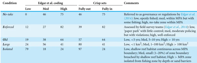
Table 1 Number of MPAs belonging to NEOLI condition sets.

Condition Edgar et al. coding Crisp sets Comments

Low Med High Fully out Fully in

No-take 0 46 75 46 75 Referred to as governance or regulations byEdgar et al. (2014): low, openly fished; med, within MPA but with some fishing; high, no-take zone within MPA

Enforced 12 27 82 39 82 Assessed by field survey teams (Edgar et al., 2014): low, ‘paper park’ with little control; med, moderate policing but with violations; high, well-enforced

Old 19 38 64 57 64 Low,<5 yrs; Med, 5–10 yrs; High>10 yrs

Large 24 56 41 80 41 Low,<1 km2; Med, 1–100 km2; High>100 km2

Isolated 79 18 24 97 24 Low, shallow reef habitat continuous across MPA boundary; Med, small (1–20%) of zone boundary breached by shallow reef habitat; High>MPA zone isolated from fishing zone by depth or sand barriers

suggesting local leadership could help mobilize a degree of restraint in local fisheries that helped ameliorate some external stressors. Together these three alternative pathways accounted for 69% of cases where successful ecological outcomes were attained.

Data coding

Case conditions and outcomes may be coded as dichotomous ‘crisp sets’ that dichoto-mously classify variables as 0 or 1 (fully out of or in a set) or as ‘fuzzy sets’ that exhibit partial membership in the set of an ideal type (Ragin, 2000).Edgar et al. (2014)originally coded the NEOLI conditions into low-medium-high categories for each variable. As the most important differences in their study was between medium and high levels of NEOLI conditions (seeFig. 3,Edgar et al., 2014), and conditions in the middle of a scale provide no additional information useful for differentiating sets in QCA (membership of 50% in a condition’s set is the point of maximum ambiguity in QCA), I aggregated low and medium levels to form crisp set definitions of NEOLI conditions (Table 1). Each condition was thus either fully in or fully out as a member of each set. This aggregation was carried out based on patterns observed inEdgar et al.’s (2014) results and prior to any QCA data analysis.

All ecological outcomes in theEdgar et al. (2014)dataset were measured during reef scuba surveys as biomass or fish species richness per 250 m2. I log-transformed (ln[n+1])

them to fuzzy set membership values in a calibration process. If fish species richness or biomass exceeded the 90th percentile for that outcome across all 121 MPAs, they were considered fully in that condition’s set of successful outcomes; if fish species richness or biomass was less than the 10th percentile, they were considered fully out of the set (Table 2). The crossover was the point where an MPA with an overall fish biomass level of 14,765 g per 250 m2would, for example, be assigned 0.50 membership in the setHigh biomass(and by implication 0.50 in a set NOT[High biomass]). There are no theoretical reasons for defining ‘high’ levels of outcomes at particular levels but some MPAs within the Reef Life Survey dataset were functionally pristine, so full set membership in a positive outcome (i.e.,>90th percentile for that condition) should indicate performance that is truly high in the range of possibilities. Note that a biomass of 120,572 g per 250 m2

(5)

Table 2 Summary of outcome set calibrations.

Outcome sets Min Mean Max Fuzzy membership calibration ln(n+1) (per 250 m2)

Fully out Crossover Fully in

High biomass 4.07 9.78 12.38 7.5 (1,808)* 9.6 (14,765) 11.7 (120,572) Total fish biomass (g)

High large fish biomass 3.11 8.54 11.79 5.5 (245) 8.1 (3,295) 10.7 (44,356) Total biomass (g) of large fish

High damselfish biomass 0.00 6.46 11.05 3.5 (33) 6.4 (602) 9.3 (10,938) Total biomass (g) of damselfish

High grouper biomass 0.00 3.36 8.74 1.0 (3) 4.5 (90) 8.0 (2,981) Total biomass (g) of groupers

High jack biomass 0.00 3.89 10.93 3.0 (20) 6.3 (518) 9.5 (13,360) Total biomass (g) of jacks

High shark biomass 0.00 2.78 11.06 0.7 (2) 5.1 (164) 9.5 (13,360) Total biomass (g) of sharks

High fish species richness 0.77 2.79 4.12 1.5 (5) 2.7 (14) 3.8 (45) All fish species

High large fish species richness 0.04 1.27 2.39 0.2 (1) 1.1 (3) 1.9 (7) Large fish (>300 mm) species

Notes.

*_{Values in parentheses denote cut-o}_ff_{and cross-over biomass and species richness values prior to ln}₍_n₊₁₎_{transformation.}

corresponds to approximately 4,800 kg per ha, a figure well in excess of values suggested as baselines to define pristine reef fish biomass (MacNeil et al., 2015).

MPAs with only one or two NEOLI conditions performed poorly and were statistically indistinguishable from fished sites (Edgar et al., 2014). The lower 10th percentile cut-off

that defined outcomes as fully outside the set of successful outcomes should thus reflect truly poor levels of MPA performance.Table 3details the coding for each MPA (starting with MPAs exhibiting all five NEOLI conditions at the top of the table, proceeding through groupings of MPAs with decreasing numbers of NEOLI conditions, and ending with those MPAs that had only a single NEOLI condition; when multiple sites from the 121 international MPA/ecoregion groupings are from a single large MPA, they are denoted, for example, as Galapagos a to Galapagos e).

Truth tables

Truth tables show the connection between all possible configurations of causal conditions that lead to an outcome of interest. The columns represent sets of causal conditions and an outcome, while the rows represent all logically possible intersections among the relevant sets. There is an exponential increase in configuration space as the number of conditions increases, with 2kideal types forkconditions. Assignment of an MPA to a configuration was based on the MPA’s membership in each condition’s set and the number of empirical instances of each output of interest was recorded for each configuration. The default inclusion level was set at 0.70 (e.g., a configuration with inclusion=0.72 would be deemed

to ‘usually’ belong to the setHigh biomass) for testing sufficiency and 0.90 for testing necessity (seeRihoux & Ragin, 2009). In truth tables, outcomes with inclusion levels in excess of the cut-offwere coded as successful (inclusion=_{1); configurations not meeting}

the cut-offwere coded as unsuccessful (inclusion=_0).

Necessary and sufficient conditions

A truth table forms a Boolean function that can be expressed as a union of fundamental set intersections, each of which corresponds to a successful outcome (Thiem & Dus¸a, 2013). If a condition is necessary for an outcome, the condition is a superset of the outcome (i.e., the

(6)

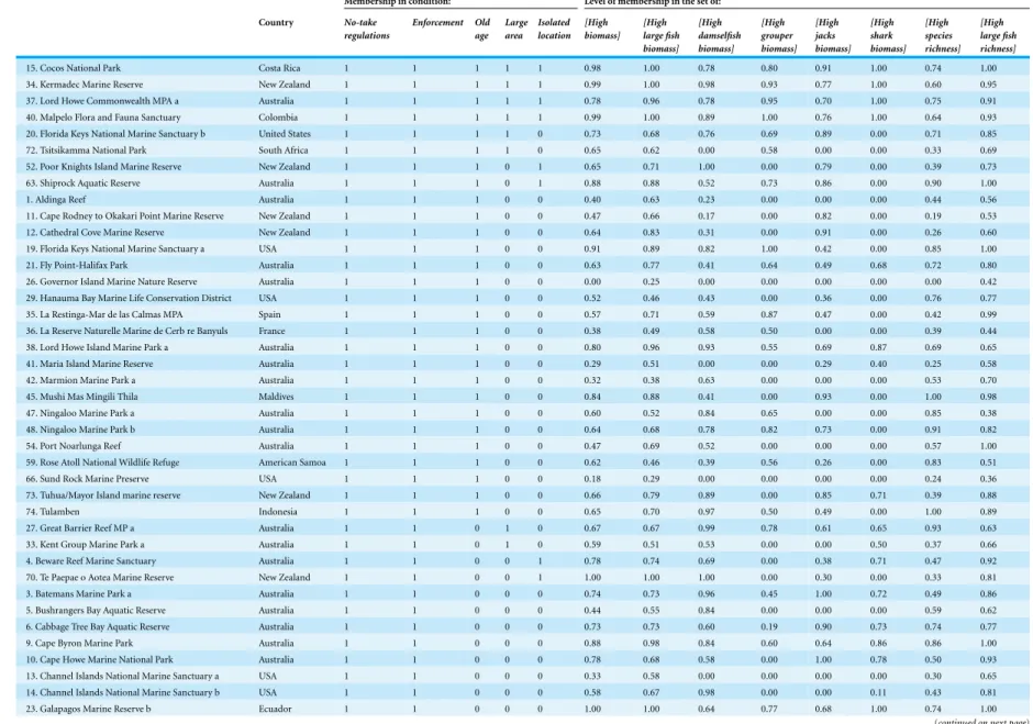
Table 3 Case study condition and outcome coding.

Membership in condition: Level of membership in the set of:

Country No-take regulations Enforcement Old age Large area Isolated location [High biomass] [High large fish biomass] [High damselfish biomass] [High grouper biomass] [High jacks biomass] [High shark biomass] [High species richness] [High large fish richness]

15. Cocos National Park Costa Rica 1 1 1 1 1 0.98 1.00 0.78 0.80 0.91 1.00 0.74 1.00 34. Kermadec Marine Reserve New Zealand 1 1 1 1 1 0.99 1.00 0.98 0.93 0.77 1.00 0.60 0.95 37. Lord Howe Commonwealth MPA a Australia 1 1 1 1 1 0.78 0.96 0.78 0.95 0.70 1.00 0.75 0.91 40. Malpelo Flora and Fauna Sanctuary Colombia 1 1 1 1 1 0.99 1.00 0.89 1.00 0.76 1.00 0.64 0.93 20. Florida Keys National Marine Sanctuary b United States 1 1 1 1 0 0.73 0.68 0.76 0.69 0.89 0.00 0.71 0.85 72. Tsitsikamma National Park South Africa 1 1 1 1 0 0.65 0.62 0.00 0.58 0.00 0.00 0.33 0.69 52. Poor Knights Island Marine Reserve New Zealand 1 1 1 0 1 0.65 0.71 1.00 0.00 0.79 0.00 0.39 0.73 63. Shiprock Aquatic Reserve Australia 1 1 1 0 1 0.88 0.88 0.52 0.73 0.86 0.00 0.90 1.00 1. Aldinga Reef Australia 1 1 1 0 0 0.40 0.63 0.23 0.00 0.00 0.00 0.44 0.56 11. Cape Rodney to Okakari Point Marine Reserve New Zealand 1 1 1 0 0 0.47 0.66 0.17 0.00 0.82 0.00 0.19 0.53 12. Cathedral Cove Marine Reserve New Zealand 1 1 1 0 0 0.64 0.83 0.31 0.00 0.91 0.00 0.26 0.60 19. Florida Keys National Marine Sanctuary a USA 1 1 1 0 0 0.91 0.89 0.82 1.00 0.42 0.00 0.85 1.00 21. Fly Point-Halifax Park Australia 1 1 1 0 0 0.63 0.77 0.41 0.64 0.49 0.68 0.72 0.80 26. Governor Island Marine Nature Reserve Australia 1 1 1 0 0 0.00 0.25 0.00 0.00 0.00 0.00 0.00 0.42 29. Hanauma Bay Marine Life Conservation District USA 1 1 1 0 0 0.52 0.46 0.43 0.00 0.36 0.00 0.76 0.77 35. La Restinga-Mar de las Calmas MPA Spain 1 1 1 0 0 0.57 0.71 0.59 0.87 0.47 0.00 0.42 0.99 36. La Reserve Naturelle Marine de Cerb re Banyuls France 1 1 1 0 0 0.38 0.49 0.58 0.50 0.00 0.00 0.39 0.44 38. Lord Howe Island Marine Park a Australia 1 1 1 0 0 0.80 0.96 0.93 0.55 0.69 0.87 0.69 0.65 41. Maria Island Marine Reserve Australia 1 1 1 0 0 0.29 0.51 0.00 0.00 0.29 0.40 0.25 0.58 42. Marmion Marine Park a Australia 1 1 1 0 0 0.32 0.38 0.63 0.00 0.00 0.00 0.53 0.70 45. Mushi Mas Mingili Thila Maldives 1 1 1 0 0 0.84 0.88 0.41 0.00 0.93 0.00 1.00 0.98 47. Ningaloo Marine Park a Australia 1 1 1 0 0 0.60 0.52 0.84 0.65 0.00 0.00 0.85 0.38 48. Ningaloo Marine Park b Australia 1 1 1 0 0 0.64 0.68 0.78 0.82 0.73 0.00 0.91 0.82 54. Port Noarlunga Reef Australia 1 1 1 0 0 0.47 0.69 0.52 0.00 0.00 0.00 0.57 1.00 59. Rose Atoll National Wildlife Refuge American Samoa 1 1 1 0 0 0.62 0.46 0.39 0.56 0.26 0.00 0.83 0.51 66. Sund Rock Marine Preserve USA 1 1 1 0 0 0.18 0.29 0.00 0.00 0.00 0.00 0.24 0.36 73. Tuhua/Mayor Island marine reserve New Zealand 1 1 1 0 0 0.66 0.79 0.89 0.00 0.85 0.71 0.39 0.88 74. Tulamben Indonesia 1 1 1 0 0 0.65 0.70 0.97 0.50 0.49 0.00 1.00 0.89 27. Great Barrier Reef MP a Australia 1 1 0 1 0 0.67 0.67 0.99 0.78 0.61 0.65 0.93 0.63 33. Kent Group Marine Park a Australia 1 1 0 1 0 0.59 0.51 0.53 0.00 0.00 0.50 0.37 0.66 4. Beware Reef Marine Sanctuary Australia 1 1 0 0 1 0.78 0.74 0.69 0.00 0.38 0.71 0.47 0.92 70. Te Paepae o Aotea Marine Reserve New Zealand 1 1 0 0 1 1.00 1.00 1.00 0.00 0.30 0.00 0.33 0.81 3. Batemans Marine Park a Australia 1 1 0 0 0 0.74 0.73 0.96 0.45 1.00 0.72 0.49 0.86 5. Bushrangers Bay Aquatic Reserve Australia 1 1 0 0 0 0.44 0.55 0.84 0.00 0.00 0.00 0.59 0.62 6. Cabbage Tree Bay Aquatic Reserve Australia 1 1 0 0 0 0.73 0.73 0.60 0.19 0.90 0.73 0.74 0.77 9. Cape Byron Marine Park Australia 1 1 0 0 0 0.88 0.98 0.84 0.60 0.64 0.86 0.86 1.00 10. Cape Howe Marine National Park Australia 1 1 0 0 0 0.78 0.68 0.58 0.00 1.00 0.78 0.50 0.93 13. Channel Islands National Marine Sanctuary a USA 1 1 0 0 0 0.33 0.58 0.00 0.00 0.00 0.00 0.30 0.65 14. Channel Islands National Marine Sanctuary b USA 1 1 0 0 0 0.58 0.67 0.98 0.00 0.00 0.11 0.43 0.81 23. Galapagos Marine Reserve b Ecuador 1 1 0 0 0 1.00 1.00 0.64 0.77 0.68 1.00 0.74 1.00

(continued on next page)

(7)

Table 3 (continued)

Country No-take regulations Enforcement Old age Large area Isolated location [High biomass] [High large fish biomass] [High damselfish biomass] [High grouper biomass] [High jacks biomass] [High shark biomass] [High species richness] [High large fish richness] 28. Great Barrier Reef MP b Australia 1 1 0 0 0 0.63 0.70 0.87 0.82 0.76 0.00 1.00 0.88 31. Jervis Bay a Australia 1 1 0 0 0 0.81 0.71 0.72 0.09 1.00 0.81 0.66 0.79 32. Jurien Bay a Australia 1 1 0 0 0 0.39 0.54 0.79 0.51 0.00 0.00 0.47 0.60 50. Point Cooke Marine Sanctuary Australia 1 1 0 0 0 0.00 0.00 0.00 0.00 0.00 0.00 0.00 0.00 51. Point Lobos State Marine Reserve USA 1 1 0 0 0 0.16 0.47 0.00 0.00 0.00 0.00 0.25 0.70 53. Port Davey National Park a Australia 1 1 0 0 0 0.00 0.07 0.00 0.00 0.00 0.42 0.00 0.17 55. Port Phillip Heads Marine National Park Australia 1 1 0 0 0 0.44 0.66 0.60 0.00 0.00 0.72 0.30 0.68 56. Port Stephens Great Lake Marine Park a Australia 1 1 0 0 0 0.71 0.57 0.69 0.25 1.00 0.68 0.67 0.70 58. Rickett’s Point Marine Sanctuary Australia 1 1 0 0 0 0.00 0.12 0.00 0.00 0.00 0.00 0.00 0.12 60. Rottnest Island a Australia 1 1 0 0 0 0.65 0.80 0.65 0.39 0.29 0.42 0.56 0.67 65. Solitary Islands Marine Park a Australia 1 1 0 0 0 0.88 1.00 0.94 0.74 0.88 1.00 0.69 0.70 71. Tinderbox Marine Reserve Australia 1 1 0 0 0 0.21 0.39 0.00 0.00 0.00 0.00 0.23 0.47 17. Ponta da Baleia-Abrolhos a Brazil 1 0 1 1 0 0.62 0.61 0.81 0.63 0.00 0.00 0.61 0.67 25. Golfo de Chiriqui Marine National Park Panama 1 0 1 1 0 0.33 0.13 0.72 0.85 0.44 0.00 0.57 0.17 43. Mnazi Bay-Ruvuma Estuary Marine Park Tanzania 1 0 1 1 0 0.59 0.34 0.78 0.67 0.00 0.00 1.00 0.70 2. Baie Ternay Seychelles 1 0 1 0 0 0.71 0.65 0.56 0.53 0.00 0.00 0.98 0.80 30. Isla de Taboga e Isla de Uraba Wildlife Refuge Panama 1 0 1 0 0 0.49 0.63 0.68 0.86 0.00 0.00 0.59 0.73 39. Machalilla Ecuador 1 0 1 0 0 0.45 0.52 0.79 0.84 0.00 0.00 0.64 0.67 49. Pangaimotu Reef MPA Tonga 1 0 1 0 0 0.38 0.40 0.77 0.94 0.00 0.00 0.90 0.12 62. Sesoko Scientific Research Area Japan 1 0 1 0 0 0.57 0.00 0.79 0.32 0.00 0.00 0.97 0.12 64. Shiraiwazaki Marine Park Japan 1 0 1 0 0 0.12 0.04 0.00 0.61 0.00 0.00 0.62 0.12 67. Table Mountain National Park a South Africa 1 0 1 0 0 0.59 0.53 0.00 0.00 0.03 0.45 0.23 0.52 68. Tawharanui Marine Reserve New Zealand 1 0 1 0 0 0.17 0.46 0.00 0.00 0.43 0.00 0.06 0.36 75. Ushibuka Marine Park Japan 1 0 1 0 0 0.40 0.24 0.57 0.75 0.00 0.00 0.66 0.29 16. Coiba National Park a Panama 1 0 0 1 1 0.76 0.85 0.80 0.91 0.85 0.57 0.69 0.71 44. Motu Motiro Hiva Chile 1 0 0 1 1 0.65 0.62 0.59 0.00 0.36 0.85 0.50 0.53 7. Caletas Costa Rica 1 0 0 1 0 0.13 0.00 0.45 0.66 0.00 0.00 0.42 0.00 8. Camaronal Costa Rica 1 0 0 1 0 0.06 0.12 0.56 0.62 0.00 0.00 0.39 0.00 18. Fiordo Comau Protected Area Chile 1 0 0 0 0 0.33 0.52 0.00 0.00 0.00 0.00 0.00 0.32 22. Galapagos Marine Reserve a Ecuador 1 0 0 0 0 1.00 1.00 0.98 1.00 0.77 1.00 0.74 1.00

(8)

Country No-take regulations Enforcement Old age Large area Isolated location [High biomass] [High large fish biomass] [High damselfish biomass] [High grouper biomass] [High jacks biomass] [High shark biomass] [High species richness] [High large fish richness] 24. Galapagos Marine Reserve c Ecuador 1 0 0 0 0 1.00 0.98 0.89 1.00 0.00 0.48 0.55 1.00 46. Ninepin Point Marine Reserve Australia 1 0 0 0 0 0.36 0.37 0.00 0.00 0.00 0.00 0.15 0.28 57. Regno di Nettuno a Italy 1 0 0 0 0 0.24 0.00 0.70 0.00 0.00 0.00 0.38 0.01 61. Seaflower Area Marina Protegida a Colombia 1 0 0 0 0 0.59 0.57 0.59 0.70 0.44 0.00 0.77 0.63 69. Te Matuku Marine Reserve New Zealand 1 0 0 0 0 0.00 0.00 0.00 0.00 0.00 0.00 0.00 0.00 101. Lord Howe Commonwealth MPA b Australia 0 1 1 1 1 0.75 0.85 0.82 1.00 0.69 0.88 0.75 0.88 80. Channel Islands National Marine Sanctuary c USA 0 1 1 1 0 0.29 0.44 0.35 0.00 0.00 0.00 0.44 0.69 81. Channel Islands National Marine Sanctuary d USA 0 1 1 1 0 0.56 0.42 1.00 0.00 0.00 0.00 0.41 0.57 86. Florida Keys National Marine Sanctuary c USA 0 1 1 1 0 0.61 0.55 0.73 0.62 0.40 0.00 0.76 0.59 104. Ningaloo Marine Park c Australia 0 1 1 1 0 0.74 0.55 0.80 0.77 0.00 0.70 0.94 0.70 105. Ningaloo Marine Park d Australia 0 1 1 1 0 0.69 0.76 0.82 0.68 0.03 0.77 0.88 0.63 78. Bonaire Netherlands

Antilles

0 1 1 0 1 0.56 0.56 0.91 0.48 0.33 0.00 0.84 0.90

87. Fly Point-Halifax Park Australia 0 1 1 0 0 0.39 0.46 0.29 0.33 0.00 0.54 0.72 0.55 102. Lord Howe Island Marine Park b Australia 0 1 1 0 0 0.66 0.79 0.93 0.07 0.43 0.78 0.62 0.59 103. Marmion Marine Park b Australia 0 1 1 0 0 0.74 0.92 0.70 0.36 0.17 0.00 0.48 0.64 106. North Sydney Harbour Aquatic Reserve Australia 0 1 1 0 0 0.64 0.69 0.81 0.00 0.85 0.29 0.66 0.66 114. Rottnest Island c Australia 0 1 1 0 0 0.56 0.68 0.73 0.40 0.43 0.70 0.55 0.68 116. Shoalwater Islands Marine Park Australia 0 1 1 0 0 0.41 0.57 0.45 0.00 0.00 0.00 0.31 0.30 118. St. Abbs and Eyemouth Marine Reserve Scotland 0 1 1 0 0 0.05 0.31 0.00 0.00 0.00 0.00 0.07 0.27 89. Galapagos Marine Reserve e Ecuador 0 1 0 1 1 0.88 0.97 0.78 0.89 0.45 0.92 0.67 1.00 112. Rose Atoll National Monument American Samoa 0 1 0 1 1 0.66 0.58 0.49 0.47 0.70 0.00 0.85 0.71 76. Batemans Marine Park b Australia 0 1 0 1 0 0.74 0.77 0.90 0.18 0.99 0.78 0.49 0.85 91. Great Barrier Reef MP c Australia 0 1 0 1 0 0.64 0.63 0.92 0.58 0.26 0.64 0.91 0.47 94. Jervis Bay b Australia 0 1 0 1 0 0.78 0.73 0.94 0.00 1.00 0.88 0.60 0.72 95. Jurien Bay b Australia 0 1 0 1 0 0.43 0.65 0.71 0.40 0.41 0.00 0.43 0.63 97. Kent Group Marine Park b Australia 0 1 0 1 0 0.53 0.49 0.58 0.00 0.00 0.44 0.40 0.67 100. Levante de Mallorca Cala Ratjada Spain 0 1 0 1 0 0.19 0.26 0.37 0.00 0.00 0.00 0.50 0.12 109. Port Stephens Great Lake Marine Park b Australia 0 1 0 1 0 0.92 0.75 0.88 0.24 1.00 0.85 0.62 0.74 117. Solitary Islands Marine Park b Australia 0 1 0 1 0 0.70 0.74 0.87 0.19 0.56 0.76 0.55 0.49 93. Illa del Toro Spain 0 1 0 0 1 0.54 0.54 0.95 0.74 0.00 0.00 0.48 0.73 79. Bronte-Coogee Aquatic Reserve Australia 0 1 0 0 0 0.55 0.55 0.67 0.00 0.62 0.00 0.63 0.64 92. Great Barrier Reef MP d Australia 0 1 0 0 0 0.58 0.50 0.81 0.71 0.00 0.00 1.00 0.70

(9)

Country No-take regulations

Enforcement Old age

Large area

Isolated location

[High biomass]

[High large fish biomass]

[High damselfish biomass]

[High grouper biomass]

[High jacks biomass]

[High shark biomass]

[High species richness]

[High large fish richness] 108. Port Davey National Park b Australia 0 1 0 0 0 0.01 0.22 0.00 0.00 0.04 0.37 0.00 0.32 110. Pupukea Marine Life Conservation District USA 0 1 0 0 0 0.30 0.21 0.30 0.00 0.00 0.00 0.63 0.36 113. Rottnest Island b Australia 0 1 0 0 0 0.32 0.39 0.71 0.62 0.00 0.00 0.58 0.62 82. Coiba National Park b Panama 0 0 1 1 1 0.85 1.00 0.71 0.94 1.00 0.80 0.65 0.73 84. Coringa-Herald Nature Reserve Australia 0 0 1 1 1 0.61 0.77 0.66 0.63 0.48 0.90 0.98 0.66 85. Ponta da Baleia-Abrolhos b Brazil 0 0 1 1 0 0.56 0.59 0.66 0.00 0.17 0.00 0.61 0.63 119. Strangford Lough Marine Nature Reserve N Ireland 0 0 1 1 0 0.00 0.00 0.00 0.00 0.00 0.00 0.00 0.00 120. Table Mountain National Park b South Africa 0 0 1 1 0 0.41 0.07 0.00 0.00 0.52 0.00 0.10 0.21 77. Beacon Island Reef Observation Area Australia 0 0 1 0 1 0.69 0.88 0.67 0.82 0.16 0.00 0.67 0.94 83. Coral Patches Reef Observation Area Australia 0 0 1 0 1 0.45 0.70 0.66 0.56 0.00 0.00 0.47 0.49 99. Leo Island Reef Observation Area Australia 0 0 1 0 1 0.65 0.72 0.72 0.59 0.00 0.00 0.60 0.77 96. Kawasan Wisata Indonesia 0 0 1 0 0 0.70 0.46 0.83 0.58 0.17 0.00 1.00 0.49 107. Panglima Laut Indonesia 0 0 1 0 0 0.62 0.30 0.79 0.56 0.00 0.00 1.00 0.21 88. Galapagos Marine Reserve d Ecuador 0 0 0 1 1 1.00 1.00 0.89 0.95 0.49 0.71 0.64 1.00 90. Galapagos Marine Reserve f Ecuador 0 0 0 1 1 0.94 1.00 0.88 1.00 0.00 0.43 0.57 1.00 98. Las Perlas Marine Special Management Zone Panama 0 0 0 1 1 0.84 0.80 0.93 0.97 0.73 0.49 0.72 0.81 111. Regno di Nettuno b Italy 0 0 0 1 0 0.15 0.00 0.67 0.00 0.00 0.00 0.41 0.01 121. Wadi El Gemal—Hamata Reserve Egypt 0 0 0 1 0 0.54 0.56 0.68 0.56 0.25 0.00 1.00 0.85 115. Seaflower Area Marina Protegida b Colombia 0 0 0 0 1 0.99 0.71 0.30 0.00 0.28 0.00 0.84 0.81

Rud

d

(2015),

P

eerJ

,

DOI

10.7717/peerj.1424

(10)

outcome occurs only in the presence of the condition). If a condition is sufficient for an outcome, the condition is a subset of the outcome (i.e., the outcome always occurs only in the presence of the condition but also in its absence).

To give a practical example, suppose that high levels of fish biomass were observed in five MPAs, two of which allowed fishing and three of which prohibited fishing: prohibition of fishing would not be a necessary condition for the positive ecological outcome. However, if in the three cases where fishing was prohibited there were three positive outcomes and no negative outcomes, a prohibition on fishing could be sufficient for achieving the positive ecological outcome.

Boolean logic is used to simplify those set relations from the truth table to as few conditions as are defensible from a theoretical or empirical perspective. The level of Boolean minimization depends on assumptions made regarding the feasibility of the ‘logical remainders’, those configurations for which there are no empirical instances, and the minimum number of empirical instances needed for a configuration to be retained in a model (setting a cut-offlevel can help dampen noisiness arising from outlying cases). I used a default frequency cut-offof two empirical instances to assess necessary and sufficient conditions. If one assumes that, if observed, none of the logical remainders would result in a positive outcome, the result is the ‘complex solution’. On the other hand, if one assumes that all logical remainders would result in a positive outcome, a ‘parsimonious solution’ with the simplest possible sufficiency conditions results. These two solutions bound the complexity of the Boolean sufficiency conditions.

In QCA models, solution coverage assesses the extent to which a particular combination of causal conditions accounts for empirical instances of an outcome (Schneider & Wagemann, 2012). For example, overall coverage of 0.75 by two sufficient conditions would mean that of all empirical observations of the outcome of interest, 75% could be explained by one or the other (or both) of the conditions. Consistency, on the other hand, refers to the degree to which cases with a shared combination of causal conditions results in an outcome of interest (Schneider & Wagemann, 2012). For example, if a sufficient condition exhibited 0.80 consistency, 80% of all the occurrences of that particular combination of conditions would lead to the outcome of interest.

Models

Sixteen models were estimated in total, one each based on the presence or negation of each of the eight sets of ecological outcomes (species richness; species richness of large (>250 mm) fish; biomass of all fish; biomass of large fish; biomass of damselfish; biomass of jacks; biomass of groupers; biomass of sharks). I used Ragin’s fsQCA software (Ragin & Davey, 2014) for all analyses.

RESULTS

With five NEOLI conditions, there were 32 possible combinations of conditions in each model. In total, 27 of the combinations had at least one empirical instance and 23 were observed at least twice and were retained for Boolean simplification (Table 4). Only four MPAs scored highly on all five NEOLI conditions; another five MPAs had various

(11)

Table 4 Number of empirical observations for each MPA configuration; configurations with no ob-servations (logical remainders) and only one observation (below cut-offfor inclusion in QCA model) are noted.

ConfigurationNo-take Enforced Old Large Isolated Instances Comments

1 1 1 1 1 1 4 All 5 NEOLI conditions

2 1 1 1 1 0 2 4 NEOLI conditions

6 1 1 0 1 1 0 Logical remainder

15 1 0 0 0 0 7 1 NEOLI condition

18 0 1 1 1 1 1 Not included in analysis

combinations of four of five possible NEOLI conditions (those nine were used byEdgar et al., 2014, as a baseline with which to compare non-fished and fished sites globally). Two configurations with four NEOLI conditions had no empirical instances and so were logical remainders in the QCA analysis.

Necessary conditions

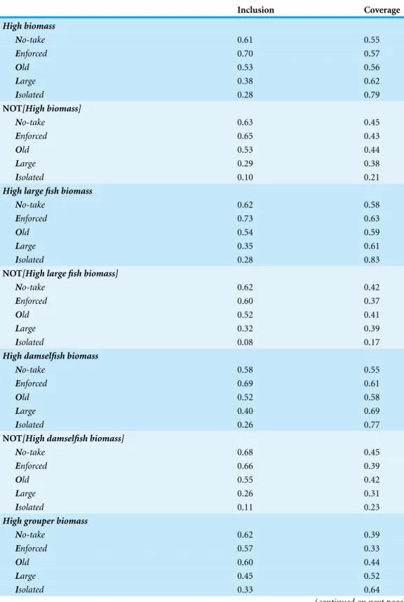
None of the five NEOLI conditions proved to be necessary for MPA ecological outcomes of interest (positive or negative) in any of the 16 models (Table 5). That is, in no case

(12)

Table 5 Tests of necessity for positive and negative ecological outcomes (must be≥0.90 to be consid-ered a necessary condition).

Inclusion Coverage

High biomass

No-take 0.61 0.55

Enforced 0.70 0.57

Old 0.53 0.56

Large 0.38 0.62

Isolated 0.28 0.79

NOT[High biomass]

No-take 0.63 0.45

Old 0.53 0.44

Large 0.29 0.38

High large fish biomass

No-take 0.62 0.58

Old 0.54 0.59

Large 0.35 0.61

NOT[High large fish biomass]

No-take 0.62 0.42

Old 0.52 0.41

Large 0.32 0.39

High damselfish biomass

No-take 0.58 0.55

Old 0.52 0.58

Large 0.40 0.69

NOT[High damselfish biomass]

No-take 0.68 0.45

Old 0.55 0.42

Large 0.26 0.31

High grouper biomass

No-take 0.62 0.39

Old 0.60 0.44

Large 0.45 0.52

(13)

NOT[High grouper biomass]

No-take 0.62 0.61

Old 0.49 0.56

Large 0.27 0.48

High jack biomass

No-take 0.66 0.35

Old 0.51 0.31

Large 0.41 0.40

NOT[High jack biomass]

No-take 0.60 0.65

Old 0.54 0.69

Large 0.30 0.60

High shark biomass

No-take 0.60 0.27

Old 0.40 0.21

Large 0.52 0.43

NOT[High shark biomass]

No-take 0.63 0.73

Old 0.58 0.79

Large 0.27 0.57

High species richness

No-take 0.59 0.54

Old 0.57 0.60

Large 0.37 0.61

NOT[High species richness]

No-take 0.66 0.46

Old 0.48 0.40

Large 0.30 0.39

(14)

High large fish species richness

No-take 0.63 0.62

Old 0.53 0.62

Large 0.34 0.63

NOT[High large fish species richness]

No-take 0.61 0.38

Old 0.52 0.38

Large 0.33 0.37

did a high level of ecological performance (or lack thereof) occur only in the presence of any single NEOLI condition. This is not unexpected given the complexity of potentially interacting factors influencing the ecological performance of MPAs.

Sufficient conditions

Model 1: High biomass

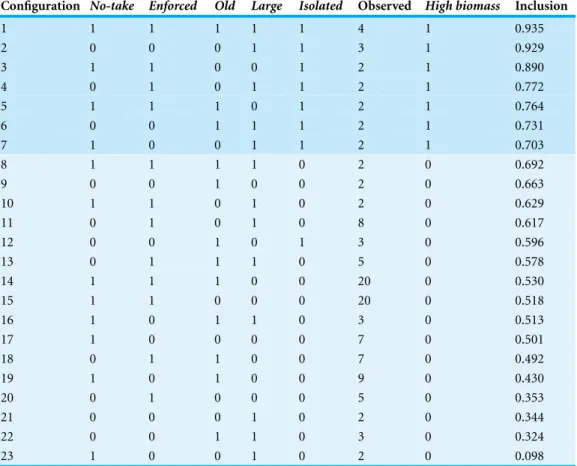
To illustrate QCA model interpretation, I present detailed results from theHigh biomass model before briefly summarizing the remaining models. Considering only configurations with two or more empirical instances each, 117 MPAs were represented in 23 NEOLI configurations. Of those, 17 cases in seven configurations exhibited inclusion levels>0.70 and were coded as members of (i.e., ‘usually in’) the setHigh biomass(Table 6). TheHigh biomassset included the configuration where all five NEOLI conditions were present and one of the two observed configurations with four NEOLI conditions. The other configuration with four NEOLI conditions (No-take,Enforced,Old,Large) fell below the cut-offneeded to ‘usually’ belong to the setHigh biomass.

In the model’s complex solution (Eq. 1.C), five different pathways, derived by Boolean manipulation of the combinations of conditions in rows 1–7 ofTable 6, were sufficient to result in high levels of fish biomass. Five conditions in each pathway are combined by logical AND operators; upper case denotes presence of condition and lower case denotes absence of a condition; dash denotes that a condition can be either present or absent;+

denotes logical OR. To illustrate, the first condition,-eoLI, can be interpreted as follows: to achieve high levels of overall fish biomass via pathway 1.C1, the MPA can be either fished or not (i.e.,Nhas no effect) AND enforcement is absent AND the MPA is not more than 10 years old AND the MPA is larger than 100 km2AND the MPA is ecologically isolated (note that this corresponds to a total of 5 MPAs in the sample, the configuration represented by rows 2 and 7 inTable 6). In aggregate, the five pathways in the complex solution in combination provided 0.211 coverage and their level of aggregate inclusion was 0.838. The five pathways themselves each provided between 0.049 and 0.078 raw coverage

(15)

Table 6 High biomasstruth table: for MPAs with at least two observations, configuration counts and degree of membership inclusion in the setHigh biomass.

Configuration No-take Enforced Old Large Isolated Observed High biomass Inclusion

1 1 1 1 1 1 4 1 0.935

2 0 0 0 1 1 3 1 0.929

3 1 1 0 0 1 2 1 0.890

4 0 1 0 1 1 2 1 0.772

5 1 1 1 0 1 2 1 0.764

6 0 0 1 1 1 2 1 0.731

7 1 0 0 1 1 2 1 0.703

8 1 1 1 1 0 2 0 0.692

9 0 0 1 0 0 2 0 0.663

10 1 1 0 1 0 2 0 0.629

11 0 1 0 1 0 8 0 0.617

12 0 0 1 0 1 3 0 0.596

13 0 1 1 1 0 5 0 0.578

14 1 1 1 0 0 20 0 0.530

15 1 1 0 0 0 20 0 0.518

16 1 0 1 1 0 3 0 0.513

17 1 0 0 0 0 7 0 0.501

18 0 1 1 0 0 7 0 0.492

19 1 0 1 0 0 9 0 0.430

20 0 1 0 0 0 5 0 0.353

21 0 0 0 1 0 2 0 0.344

22 0 0 1 1 0 3 0 0.324

23 1 0 0 1 0 2 0 0.098

individually; unique coverage for each pathway ranged from 0.021 to 0.055 and inclusion levels ranged from 0.827 to 0.878.

-eoLI+_n-oLI+_ne-LI+NE_-lI+NEO_-I→_{High biomass}. (1.C)

With the exception ofIsolated, the conditions that formed pathways toHigh biomass could have either positive or negative effects on overall fish biomass depending on the context in which they occurred. While it may at superficially appear thatIsolated is necessary forHigh biomassoutcomes (becauseIsolatedappears in each of the five pathways that combine to lead toHigh biomass), recall that the definition of a necessary condition is that it is a superset of the outcome: the outcome only appears in the presence of the condition.Table 6showed, however, that row 12 (neOlI) had three empirical instances whereHigh biomasswas not achieved even though the MPAs were isolated; ifIsolatedwere a necessary condition, these MPAs would also have exhibited aHigh biomassoutcome. Neither can one say thatIsolatedis sufficient, on its own, to lead to positive outcomes. Considering only cases whereHigh biomasswas observed—the first seven rows ofTable 6—Isolatedappears in all configurations but never on its own, only in

(16)

combination with other conditions in the seven distinct MPA configurations that lead to High biomass. Eight of nine logical remainders includedIsolated, further highlighting the potential nuance of the role of ecological isolation—the complex solution assumes that none of the logical remainders would, if actually observed, result in high biomass (a point we return to in the Discussion).

Solution (1.C) exhibited configurational complexity in that multiple alternative pathways led to a single outcome of interest. The first three pathways comprising the complex solution highlighted that large, isolated MPAs could compensate, in terms of overall production of fish biomass, for some fishing within MPAs or in the face of weak enforcement, even in young MPAs. Pathways three and four implied thatLargeand the combination ofNo-takeandEnforcedwere substitutes in the production of high levels of fish biomass within MPAs.

When the five pathways in the complex solution were simplified as much as possible with Boolean logic (i.e., assuming all logical remainders, if actually observed, would result inHigh biomass), the parsimonious solution (1.P) consisted of two pathways sufficient for achieving high levels of fish biomass within MPAs:

LI+EI→_{High biomass} _(1.P)

Based on the ecological performance of the 17 MPAs that surpassed a reasonable threshold that qualified them as members of the setHigh biomass, ecological isolation in combination with either large area or effective enforcement were the simplest configurations that led toHigh biomasson a consistent basis. MPAs needed have only two NEOLI conditions and neither solution involved the presence of eitherNo-takeorOld. Moving from the complex to parsimonious solution increased coverage slightly from 0.211 to 0.238 and reduced inclusion from 0.838 to 0.804. The parsimonious pathways did not demonstrate the same level of subtlety as did the more stringent complex model. In the complex solution, a total of 17 specific MPAs were covered by the five sufficient pathways leading toHigh biomass(Table 7). A total of 20 MPAs were covered under the less stringent parsimonious solution.

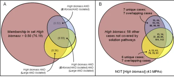
There were 14 cases with greater than 0.50 membership in pathwayLI[LargeAND Isolated], 13 cases with greater than 0.50 membership were covered by pathwayEI [EnforcedANDIsolated], and an overlap of 7 cases.Figure 1Ashows an area-proportional Venn diagram (Micallef & Rodgers, 2014) with the setHigh biomassnormalized to 100%. Solution coverage was 0.238 (0.065+_0.089+_{0.084): the two solution pathways covered}

23.8% of the area the setHigh biomassand the solution inclusion was 0.804 (i.e., 19.6% of the area of the two sufficient pathways fell outside of theHigh biomassset, in the set NOT[High biomass]). InFig. 1B, the MPAs are mapped onto the sets of conditions and outcome. Low coverage left much of the set ofHigh biomassunexplained and implies other conditions and sufficiency pathways are important in explaining high levels of overall fish biomass at the 121 MPAs.

A more stringent consistency cut-offin the model would constrain solution boundaries. For example, increasing the inclusion cut-offto 0.85 in the first stage of the modeling

(17)

Table 7 MPAs with greater than 50% membership in the sufficient conditionHigh biomass.

Case Complex Parsimonious

1.C1 1.C2 1.C3 1.C4 1.C5 1.P1 1.P2

4. Beware Reef Marine Sanctuary 1 1

15. Cocos National Park 1 1 1

16. Coiba National Parkb 1 1

34. Kermadec Marine Reserve 1 1 1

37. Lord Howe Commonwealth MPAa 1 1 1

40. Malpelo Flora and Fauna Sanctuary 1 1 1

44. Motu Motiro Hiva 1 1

52. Poor Knights Island Marine Reserve 1 1 1

63. Shiprock Aquatic Reserve 1 1 1

70. Te Paepae o Aotea Marine Reserve 1 1

78. Bonaire 1

82. Coiba National Park 1 1

84. Coringa-Herald Nature Reserve 1 1

88. Galapagos Marine Reserved 1 1 1 1

89. Galapagos Marine Reservee 1 1 1

90. Galapagos Marine Reservef 1 1 1 1

93. Illa del Toro 1

98. Las Perlas Marine Special Management Zone 1 1 1 1

101. Lord Howe Commonwealth MPA b 1 1

112. Rose Atoll National Monument 1 1 1

Notes.

Italics indicate MPAs not covered in the complex solution but covered under the parsimonious solution.

Figure 1 Parsimonious solution forHigh biomassoutcomes: (A) solution coverage by each of two pathways sufficient to achieveHigh biomass; and (B) specific MPAs that are members of pathways.

(18)

Figure 2 Venn diagram of solution coverage for model 2, NOT[High biomass].

process (i.e., imposing a more stringent definition of ‘usually in’ the setHigh biomass) would reduce the number of cases used in the Boolean analysis to nine empirical instances (coverage=0.145) arising from three di_fferent configurations of MPA conditions (all still

involvingIsolated).

Model 2: NOT[High biomass]

In addition to analysis of positive ecological outcomes from MPAs, the QCA analysis in the second model identified sufficient conditions needed to lead to set negation, the set of all MPAs belonging to NOT[High biomass]. Two cases in a single configuration exhibited consistency levels>0.70 and were coded as members of the set NOT[High biomass]. The complex solution could not be simplified, coverage was 0.034, and a single pathway (Eq. 2.C/2.P) described a sufficient condition leading to the absence of high levels of fish biomass:

N_eoL_i→_{NOT[High biomass]} (2.C/2.P)

This pathway consisted of a very specific configuration involving all five conditions (2 present, 3 absent) and had only two empirical instances, the Costa Rican Caletas (row 7) and Camaronal (row 8) MPAs. NEOLI conditions played an extremely limited role in explaining pathways to low levels of overall fish biomass (Fig. 2). Some 97% of low biomass outcomes could not be explained by this solution, implying that other pathways not dependent on either the presence or absence of NEOLI conditions explained low levels of fish biomass (note the striking contrast in low biomass outcomes when comparing all fish species to commercially exploited species—see models 8, 10, and 12 below).

(19)

Model 3: High large fish biomass

The complex solution (3.C) consisted of five pathways sufficient to lead toHigh large fish biomass.Table 8shows model diagnostics for all parsimonious solutions leading to positive ecological outcomes. The parsimonious solution (3.P) consisted of a single pathway comprised of a single condition, ecological isolation. Three MPAs that were not part of the complex solution (78. Bonaire; 101. Lord Howe Commonwealth MPA b; 115. Seaflower Area Marina Protegida b) were part of the parsimonious solution simply by virtue of their ecological isolation.

neO_-I+-eoLI+n-oLI+NE_-lI+NEO_-I→_{High large fish biomass} (3.C)

—-I→High large fish biomass (3.P)

Model 4: NOT[High large fish biomass]

In total, seven MPAs were used to calculate a parsimonious solution (4.P) that included two sufficient pathways to membership in NOT[High large fish biomass](Table 9shows parsimonious solutions for all negated models; all complex solutions are available from the author upon request). In model 4, the parsimonious and complex solutions (4.C) coincided as no Boolean simplifications were possible. Note that, contrary to received wisdom about MPA size,Largefigured in both sufficient pathways to low biomass outcomes; but recall it was also a condition in two pathways toHigh large fish biomass, demonstrating that the effect of MPA size was highly context dependent.

-eoL_i+ne-L_i→NOT[High large fish biomass] (4.P/4.C)

Models 5–16

The remaining models for various ecological outcomes are outlined inTables 8and9. Note that in Model 8 a total of 40 cases in seven configurations were coded as members of the negated set NOT[High grouper biomass].This was the first model to achieve over 0.50 coverage, where four sufficient pathways in the parsimonious solution accounted for over half of all observed MPAs with low levels of grouper biomass. Similarly, 42 cases (coverage

=_{0.542) in Model 10 and 54 cases in Model 12 (coverage}=_{0.706) were coded as members}

of the negated sets NOT[High jack biomass]and NOT[High shark biomass], respectively. For all three commercially-targeted species, negated solutions had much higher coverage levels compared to more general biomass or species richness outcomes. Lack of ecological isolation was an important factor in virtually all solution pathways (Table 9).

DISCUSSION

This study identified pathways that led from MPA design and management conditions to MPA performance, measured in terms of fish species richness and biomass for all fish, large fish, and specific groups of species (damselfish, groupers, jacks, sharks). The results demonstrated the importance of considering ecological and managerial conditions in the MPA design and implementation process. In addition to the substantive results, this study demonstrated the potential utility of QCA and set theory to assess the determinants of

(20)

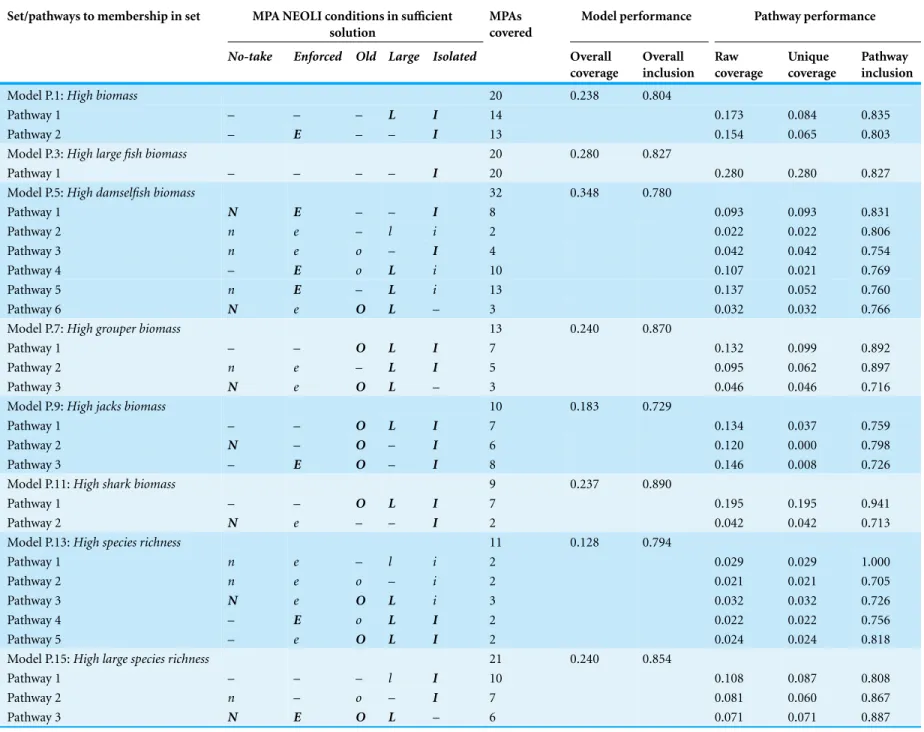
Table 8 Summary of parsimonious QCA solutions for positive outcomes (conditions, performance, and total coverage of MPAs by pathway and models). Set/pathways to membership in set MPA NEOLI conditions in sufficient

solution

MPAs covered

Model performance Pathway performance

No-take Enforced Old Large Isolated Overall

coverage

Overall inclusion

Raw coverage

Unique coverage

Pathway inclusion

Model P.1:High biomass 20 0.238 0.804

Pathway 1 – – – L I 14 0.173 0.084 0.835

Pathway 2 – E – – I 13 0.154 0.065 0.803

Model P.3:High large fish biomass 20 0.280 0.827

Pathway 1 – – – – I 20 0.280 0.280 0.827

Model P.5:High damselfish biomass 32 0.348 0.780

Pathway 1 N E – – I 8 0.093 0.093 0.831

Pathway 2 n e – l i 2 0.022 0.022 0.806

Pathway 3 n e o – I 4 0.042 0.042 0.754

Pathway 4 – E o L i 10 0.107 0.021 0.769

Pathway 5 n E – L i 13 0.137 0.052 0.760

Pathway 6 N e O L – 3 0.032 0.032 0.766

Model P.7:High grouper biomass 13 0.240 0.870

Pathway 1 – – O L I 7 0.132 0.099 0.892

Pathway 2 n e – L I 5 0.095 0.062 0.897

Pathway 3 N e O L – 3 0.046 0.046 0.716

Model P.9:High jacks biomass 10 0.183 0.729

Pathway 1 – – O L I 7 0.134 0.037 0.759

Pathway 2 N – O – I 6 0.120 0.000 0.798

Pathway 3 – E O – I 8 0.146 0.008 0.726

Model P.11:High shark biomass 9 0.237 0.890

Pathway 1 – – O L I 7 0.195 0.195 0.941

Pathway 2 N e – – I 2 0.042 0.042 0.713

Model P.13:High species richness 11 0.128 0.794

Pathway 1 n e – l i 2 0.029 0.029 1.000

Pathway 2 n e o – i 2 0.021 0.021 0.705

Pathway 3 N e O L i 3 0.032 0.032 0.726

Pathway 4 – E o L I 2 0.022 0.022 0.756

Pathway 5 – e O L I 2 0.024 0.024 0.818

Model P.15:High large species richness 21 0.240 0.854

Pathway 1 – – – l I 10 0.108 0.087 0.808

Pathway 2 n – o – I 7 0.081 0.060 0.867

Pathway 3 N E O L – 6 0.071 0.071 0.887

Notes.

Uppercase/bold denotes presence required; lowercase denotes absence required (i.e., NOT set member); dash denotes condition may be present or absent.

Rud

d

(2015),

P

eerJ

,

DOI

10.7717/peerj.1424

(21)

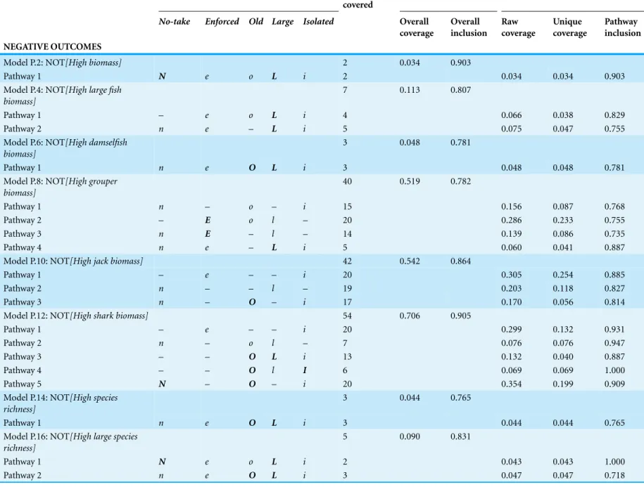
Table 9 Summary of parsimonious QCA model solutions for negated models: conditions, performance, and total coverage of MPAs by pathway and models. Set/pathways to membership in set MPA NEOLI conditions MPAs

covered

Model performance Pathway performance

No-take Enforced Old Large Isolated Overall

coverage

Overall inclusion

Raw coverage

Unique coverage

Pathway inclusion NEGATIVE OUTCOMES

Model P.2: NOT[High biomass] 2 0.034 0.903

Pathway 1 N e o L i 2 0.034 0.034 0.903

Model P.4: NOT[High large fish biomass]

7 0.113 0.807

Pathway 1 – e o L i 4 0.066 0.038 0.829

Pathway 2 n e – L i 5 0.075 0.047 0.755

Model P.6: NOT[High damselfish biomass]

3 0.048 0.781

Pathway 1 n e O L i 3 0.048 0.048 0.781

Model P.8: NOT[High grouper biomass]

40 0.519 0.782

Pathway 1 n – o – i 15 0.156 0.087 0.768

Pathway 2 – E o l – 20 0.286 0.233 0.755

Pathway 3 n E – l – 14 0.139 0.086 0.735

Pathway 4 n e – L i 5 0.060 0.041 0.887

Model P.10: NOT[High jack biomass] 42 0.542 0.864

Pathway 1 – e – – i 20 0.305 0.254 0.885

Pathway 2 n – – l – 19 0.203 0.118 0.827

Pathway 3 n – O – i 17 0.170 0.056 0.814

Model P.12: NOT[High shark biomass] 54 0.706 0.905

Pathway 1 – e – – i 20 0.299 0.132 0.931

Pathway 2 n – o l – 7 0.076 0.076 0.947

Pathway 3 – – O L i 13 0.132 0.040 0.887

Pathway 4 – – O l I 6 0.069 0.069 1.000

Pathway 5 N – O – i 20 0.354 0.199 0.909

Model P.14: NOT[High species richness]

3 0.044 0.765

Pathway 1 n e O L i 3 0.044 0.044 0.765

Model P.16: NOT[High large species richness]

5 0.090 0.831

Pathway 1 N e o L i 2 0.043 0.043 1.000

Pathway 2 n e O L i 3 0.047 0.047 0.718

Rud

d

(2015),

P

eerJ

,

DOI

10.7717/peerj.1424

(22)

MPA performance and, more generally, how set theoretic approaches to ecological success may complement and extend insights from statistical analyses.

Conditions and configurations influencing ecological success

One of the five NEOLI conditions—ecological isolation—was pivotal for positive ecological outcomes relating to species richness of large fish and biomass of all fish, of large fish only, and of three commercially exploited fishes (groupers, jacks and sharks). Isolation was in fact, on its own, sufficient for leading to high biomass of large fish in the parsimonious solution.Isolatedwas present in 12 of 14 pathways to positive ecological performance in parsimonious solutions (Table 8) and NOT[Isolated]was not present in any. For complex solutions (available from the author upon request),Isolatedwas present in 20 of 22 pathways to positive ecological performance (NOT[Isolated]was present in only one solution). Conversely, in the negated models examining conditions influencing poor MPA performance, NOT[Isolated]was present in 14 of 17 pathways in parsimonious solutions (Table 9) (Isolatedwas present in one solution) and 17 of 21 in complex solutions.

Edgar et al. (2014)found that ecological isolation was important, seeming to “exert a stronger influence for community-level biomass and richness metrics than the other four features. . . (and that) although very important, the effect of isolation was similar in magnitude—rather than clearly superior—to other MPA features for biomass of sharks, groupers and jacks” (p. 218). QCA results instead suggest that ecological isolation is clearly the most important factor affecting ecological performance. The importance of isolation aligns well with insights from ecological models of MPAs (e.g.,White et al., 2011).

Other areas of discrepancy between the statistical and set-theoretic models included the importance of: no-take regulations in the production of overall fish biomass (not part of QCA pathways to success in the parsimonious solutions and conflicting in direction in the complex solutions); MPA age being related to higher levels of jack biomass; and the effects ofNo-takeandEnforcedon species richness in MPAs (QCA results suggested thatOldand Isolatedalso play important contextual roles). On other ecological outcomes, however, the approaches converged. For example, both statistical and set theoretic approaches identified lack of enforcement as being associated with relatively low levels of grouper biomass and identified the role of old MPAs in the production of high levels of shark biomass.

All conditions other than ecological isolation could positively or negatively affect positive ecological outcomes for large species diversity and biomass measures, thus highlighting the importance of context on success. Large MPAs appeared to, on balance, be important for positive outcomes and older MPAs appeared to be more important for commercially landed species compared to large species in general. MPA no-take regulations and enforcement did not have any degree of clear directional influence on ecological outcomes; in particular theNEOcombination (row 14,Table 6), comprising 20 observations, had no positive or few minor negative impacts on ecological performance. Figure 3illustrates all possible overlapping set combinations for the five NEOLI conditions and the number of empirical instances for each configuration. MPA performance,

(23)

Figure 3 Count of MPAs exhibiting various combinations of conditions.Gray fill indicates configu-rations that were absent or observed at only a single site in the Reef Life Survey dataset. The colored configurations indicate the difference in times that particular configurations were present in parsimo-nious solutions less the times they appeared in negative solutions: blue fill indicates top performing MPA configurations (positive minus negative outcomes= +5,+6 or+7); green,+2,+3 or+4; yellow,−1, 0 or+_{1; orange,}−_4,−_{3 or}−_{2; and red,}−_5,−_{6 or}−_7.

measured as the difference in the number of times a NEOLI condition was part of positive and negative parsimonious solutions, suggests that MPA ecological outcomes were broadly mediocre in the absence of ecological isolation.

Overall, NEOLI conditions played a relatively limited role in sustaining high levels of ecological performance in MPAs. Solution coverage ranged from 0.128 for the species richness model to 0.348 for the damselfish biomass model, implying that 65% or more of positive ecological outcomes observed in the field could not be explained in terms of NEOLI conditions alone or in combination. On the other hand, the higher levels of coverage in the negated models of jack (0.542), grouper (0.519) and shark (0.706) biomass lends support for the perspective that MPAs may provide performance asymmetries and be more effective in preventing further declines in large fish biomass relative to rebuilding biomass towards levels seen in near-pristine conditions. Among the negated models, there were large differences in solution coverage between biomass outcomes for the large commercially-exploited species and the more general biomass and species richness models. This hints that there may be potential economic benefits for capture fisheries and tourism (for wildlife viewing) from conservation-oriented MPAs that provide insurance against declines in biomass of relatively mobile large species.

(24)

For damselfish biomass, biomass levels for all fish, and for large fish only, and for both species richness metrics, the negated models only covered 3%–11% of all negative outcomes. For the models with low coverage, the implication is that conditions other than the NEOLI conditions account for the vast majority of MPA buffering capacity against adverse ecological outcomes. A wide variety of other conditions have been identified as potentially important for MPA and small-scale fisheries management; some possible candidates include fishing community leadership, residents’ perceptions regarding threats to fish stocks, the availability of alternative livelihood opportunities, high levels of community engagement, management accountability, social capital and trust among community members, and outside (e.g., NGO) support for local management (e.g.,

Guti´errez, Hilborn & Defeo, 2011;Pollnac, Crawford & Gorospe, 2001;Rudd et al., 2003;

Warner & Pomeroy, 2012;Sutton & Rudd, 2015). Given the variability even among the eight indicators used in this study, it may also be the case that NEOLI conditions positively affect levels of alternative performance metrics. Many ecological indicators of MPA success are possible (Soykan & Lewison, 2015) and futher investigation would be needed to clarify the relationship between NEOLI conditions and a broader suite of ecological outcomes. The disparities in QCA coverage for different ecological metrics highlights the difficulties in relying on MPAs as robust tools for providing multiple types of conservation benefits simultaneously. MPAs may need to be explicitly focused on particular conservation goals rather than being implemented with unrealistic expectations that they can be ‘all things for all people’. Indeed, over a decade agoAgardy et al. (2003)cautioned that if MPAs failed to live up to unrealistically high expectations, there could be repercussions for marine conservation if managers were to lose confidence in MPAs as an effective tool in the overall conservation toolkit.

QCA utility for MPA studies

Set-theoretic methodologies have been used over the past 20 years to identify causal pathways from case conditions to outcomes of interest for a diverse range of social and political phenomena. Increasingly QCA has been applied in other fields such as the health sciences (Candy et al., 2013), public and social policy (Rihoux & Marx, 2013), and environmental management (Basurto, 2013;Huntjens et al., 2011;Never & Betz, 2014;

Robinson, Holland & Naughton-Treves, 2014;Rudel, 2008;Sutton & Rudd, 2015). If used in conjunction with statistical and qualitative research, set-theoretic methods also have potential to help bridge the quantitative and qualitative research worlds (Brady & Collier, 2004;Goertz & Mahoney, 2012;Rihoux, 2003).

While beyond the scope of the current study, it would be possible to delve more deeply into context at MPAs that have been flagged as having potentially anomalous performance given their NEOLI configuration and develop hypotheses about which additional conditions, if empirically present, may or may not lead to outcomes of interest. Individual cases identified as logical remainders or contradictions in QCA can provide rich insights to help interpret Boolean solutions and can complement statistical analyses even in large-nstudies (Glaesser & Cooper, 2011) by helping advance theoretical insights