Optimization of filling systems for low pressure by Flow 3D

José Miguel Gonçalves Ledo Belo da Costa

Optimization of filling systems

for low pressure by Flow 3D

José Miguel Gonçalves Ledo Belo da Costa

Op

timization of filling sys

tems for lo w pr essur e b y Flo w 3D

Universidade do Minho

Escola de Engenharia

Dissertação de Mestrado

Ciclo de Estudos Integrados Conducentes ao

Grau de Mestre em Engenharia Mecânica

Trabalho efectuado sob a orientação do

Doutor Hélder de Jesus Fernades Puga

Professor Doutor José Joaquim Carneiro Barbosa

José Miguel Gonçalves Ledo Belo da Costa

Optimization of filling systems

for low pressure by Flow 3D

Universidade do Minho

A

CKNOWLEGMENTS

I express my deep gratitude and admiration to Doctor Hélder Puga

for the constant motivation that passed me, the high scientific skills and that it has and tried to pass on during this work. His constant availability, your encouragement, your friendship, your confidence and your support greatly contributed to the dissertation presented here. My sincere thanks

To Professor Doctor Joaquim Barbosa

the constant availability, your encouragement, your friendship, your confidence and your support greatly contributed to the thesis presented here.

To DEM,

the availability of all possible resources to this work.

I would also like to express my gratitude to a group of people, which encouraged me, doing better every day: To CINFU particularly to Engineer Paulo Aguiar

the enormous availability and permanent advice throughout my scientific path, their assistance in the experimental step was precious to the culmination of this work.

To Engineer Raul Truchado

the assistance given and high availability to meet my questions and having the critical spirit that fostered the rapid developed in the short time that we were in contact.

To Engineer José Atilano

companion in this path, my thanks for all the cooperation, friendship and to all conversations and discussions that helped me grow through the academic live and for all the help invested in this work. I wish you success

iv

To João Viana

my thanks for all the support, cooperation, friendship

and for all the time and dedication invested in helping me throughout this path.

To my colleagues at the University of Minho,

i thank your companionship given in these academic live.

Highlighting those who followed me closely throughout this journey.

My parents and my grandparents

who contributed their efforts and support for the realization

to this personal goal. Without their help I wouldn’t be able to achieve this goal. A special thanks to them.

To all,

A

BSTRACT

As part of the dissertation and bearing in mind the parameters in which the possibility of a choice of tutor and the subject to be addressed is established, the subject for development

’Optimization of filling systems for low pressure by Flow 3D ®_{’ was chosen. For this it was}

necessary to define the objectives to achieve and the methods to attain them.

Despite the wide range of software able to simulate and validate filling systems, Flow 3D® has been shown as one of the best tools in the market, demonstrating its ability to simulate with distinctive accuracy with respect to the entire process of filling and the behavioral representation of the fluid obtained. To this end, it is important to explore this tool for a better understanding of the processes involved and to serve as an exploratory basis for the simulation of filling systems, simulation being one of the great strengths of the current industry due to the need to reduce costs and time waste, in practical terms, that lead to the perfecting of the dimensioning of filling devices, which are reflected in delays and wasted material.

In this way it is intended to validate the methodology to design a filling system in low-pressure casting process, exploring their physical models and thus allowing for its characterization. For this, consider the following main phases: The exploration of the simulation software Flow 3D®; modeling of filling systems; simulation, validation and optimization of systems modeled by exploring the parameters of the models. Therefore, it is intended to validate the pressure curves under study and the eventual mining of the most relevant information in a casting analysis. The pressure curves that were used were obtained through the gathered literature and the practical work previously performed. Through the results it was possible to conclude that the pressure curve with 3 levels meets the intended purpose of a laminar filling regime and associated speeds never exceeding 0.5 𝑚/𝑠. The pressure curve with 2 filling levels has a more turbulent system, having filling areas with velocities above 0.5 𝑚/𝑠. The heat transfer parameter was studied due to the values previously obtained didn’t corroborate the behavior of dissipation regarding to the casting. In this way, new values, more in tune with the casting process, were obtained. The achieved results were compared with those generated by NovaFlow & Solid®, which were shown to be similar, validating the parameters established in the simulations. Flow 3D® was proven a powerful tool for the simulation of casting parts.

R

ESUMO

Como parte da dissertação tendo em mente os parâmetros onde está estabelecida e tendo em conta os moldes estipulados, permitiram a escolha do orientador bem como do tema a abordar. Optou-se pelo desenvolvimento do tema 'Otimização de sistema de enchimento para baixa pressão no software Flow 3D®'. Para isso foi necessário definir os objectivos a atingir e os métodos para alcançá-los.

Apesar da ampla gama de software capazes de simular e validar sistemas de gitagem, o Flow 3D® tem-se revelado como uma das melhores ferramentas do mercado, evidenciando a capacidade de simular com maior rigor no que respeita a todo o processo de enchimento de cavidades. Para tal, torna-se importante a exploração desta ferramenta para uma melhor compreensão das metodologias envolvidas e como base exploratória para a simulação de sistemas de enchimento, sendo a simulação um dos grandes trunfos da indústria atual, face à necessidade de diminuição de custos e de desperdício de tempo no aperfeiçoamento prático do dimensionamento dos sistemas de enchimento, que se refletem em atrasos e em desperdício de material.

Desta forma pretende-se validar uma metodologia de projeto dum sistema de enchimento através do processo de fundição de baixa pressão, explorando as capacidades e modelos matemáticos do Flow 3D®. Para isso, consideraram-se as seguintes fases principais: modelação, discretização do modelo; simulação, validação e otimização de sistemas modelados explorando os parâmetros dos mesmos. De forma a simular o enchimento da cavidade moldante, utilizaram-se curvas de pressão obtidas através da bibliografia e de trabalhos práticos previamente realizados. Pelos resultados obtidos foi possível concluir que uma curva de pressão com 3 patamares se encontra em regime de enchimento laminar, com velocidades associadas nunca superiores a 0.5 𝑚 𝑠⁄ .Na curva de pressão com 2 patamares o regime de enchimento é mais turbulento, havendo zonas de enchimento com velocidades acima dos 0.5 𝑚 𝑠⁄ . O parâmetro de transferência de calor, full energy, foi estudado devido aos valores obtidos inicialmente não corroborarem com comportamento da dissipação face à fundição. Assim, foram obtidos valores consensuais com a prática de fundição. Compararam-se os resultados obtidos com resultados gerados pelo NovaFlow & Solid®,que se mostraram idênticos, validando deste modo os parâmetros relativos às simulações. O Flow 3D® revelou-se uma ferramenta poderosa faceà simulação de elementos de fundição.

C

ONTENT

Acronyms and Abbreviations List ... xvii

1. Introduction ... 1

1.1 Aim of the Dissertation... 1

1.2 Methodology of the Dissertation ... 2

1.3 Layout of the Dissertation ... 2

1.4 Scope of the Dissertation ... 3

2. State of the Art ... 5

2.1 Low Pressure ... 5

2.1.1 Advantages and Disadvantages ... 7

2.2 Essential Parameters of the Low Pressure Casting ... 9

2.2.1 Mold Temperature ... 9

2.2.2 Pre-heating of the mold ... 10

2.2.3 Temperature of Liquid Metal ... 10

2.2.4 Pressure Needed to Pressurize the Molten Metal ... 10

2.2.5 Stabilization Pressure ... 12

2.2.6 Alloys Used in Low Pressure Casting ... 12

2.3 CAE in Casting ... 13

2.4 Computational Fluid Dynamics (CFD) methods ... 15

2.4.1 Finite Difference Method ... 16

2.4.2 The Finite Element Method ... 17

2.5 Construction of the Model ... 18

x

3.1 Introduction ... 21

3.2 Governing Equations ... 21

3.3 Control Volume Approach ... 23

3.4 Volume-of-Fluid Method ... 26

3.5 Construction of the Geometric Model ... 28

3.6 Meshing ... 29

3.7 Boundary Conditions ... 31

3.8 Physical Models ... 32

4. Numerical Simulation ... 35

4.1 Model Definition (CAD) ... 35

4.2 Numerical Definition ... 37

4.3 Modifications ... 41

4.4 Final Simulations ... 47

4.5 Software simulation comparisions ... 61

5. Conclusions and Future Prospects ... 63

5.1 Conclusion ... 63

5.2 Future Prospects ... 65

Bibliography ... 67

Attachment I – Boundary Conditions ... 71

L

IST OF

F

IGURES

Chapter 1

Figure 1.1 - Design cycle ... 1

Chapter 2

Figure 2.2 - Example of low pressure casting using sand molds ... 7

Figure 2.3 - Cycle of digital data... 14

Figure 2.4 - CFD software ... 18

Chapter 3

Figure 3.2 - Fractional area representation ... 24

Figure 3.3 - Example of cases where a single mesh block is not efficient ... 25

Figure 3.4 - (a) Example of linked blocks, (b) Example of nested blocks ... 25

Figure 3.5 - Interaction between fluids ... 26

Figure 3.6 - Representation of the VOF method ... 26

Figure 3.7 - TruVOF representation ... 27

Figure 3.8 - (a) Geometric model, (b) Meshed model, (c)Favorized mode ... 29

Figure 3.9 - Application of the fixed points ... 30

Figure 3.10 - Errors from rough mash grids ... 30

Figure 3.11 - Mesh with open volume ... 31

Figure 3.12 - Symmetric boundary ... 31

Figure 3.13 - (a) Air entrainment parameters, (b) Bubble and phase change parameters ... 32

Figure 3.14 - (a) Gravity and non-inertial reference frame parameters, (b) Heat transfer parameters ... 33

xii

Chapter 4

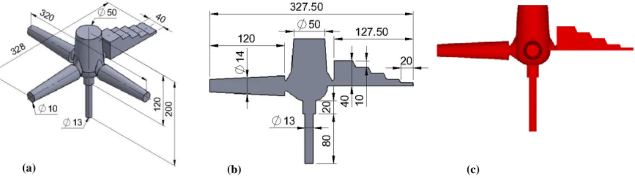
Figure 4.1 - Measurement on Geometric model used in the simulation ... 35

Figure 4.2 - (a) Geometric model, (c) Flow 3D® model regarding different components (Blue – Hole, Red . Solid) ... 36

Figure 4.3 - (a) Part for final simulation, (b) section view (c) Flow 3D® model ... 36

Figure 4.4 - Methodology flowchart ... 37

Figure 4.5 - Solid properties from the sand mold ... 38

Figure 4.6 - (a)Favorized part with 7mm size mesh, (b) Favorized full model, with 11mm size mesh ... 39

Figure 4.7 - (a) Favorized part with smaller mesh size, (b) Favorized full model with smaller mesh size ... 39

Figure 4.8 – Simulated part with mesh of symmetric boundary conditions and pressure boundary condition in the entry of the molten metal ... 40

Figure 4.9 - Test curve pressure to obtain a fully functional simulation ... 41

Figure 4.10 – Simulation without the z max open volume ... 41

Figure 4.11 - Fill fraction graph of simulation without the z max open volume ... 41

Figure 4.12 - Pressure boundary condition to z maximum open volume ... 42

Figure 4.13 - Fill fraction with z maximum open volume ... 42

Figure 4.14 - Pressure simulation of z maximum open volume ... 42

Figure 4.15 - Model with virtual valve to simulate the permeability capacity of the mold enabling the output of gases to the atmosphere ... 43

Figure 4.16 - Valve parameters used to simulate the permeability of the mold ... 43

Figure 4.17 - Fill fraction graph with model with virtual valve ... 43

Figure 4.18 - Simulation with virtual valve to simulate the permeability of the mold ... 44

Figure 4.19 - Fill fraction graph with 2mm mesh size ... 44

Figure 4.20 - Simulation with 2mm mesh size ... 44

Figure 4.21 - (a) Favorized part with 4mm mesh size, (b) Favorized part with 2 mm mesh size ... 45

Figure 4.22 - Model with virtual valves to simulate the permeability of the mold regarding the entry zones of molten metal ... 45

Figure 4.23 - Simulation with valves ... 46

Figure 4.24 - Model with virtual valves in the extremities of the geometries to simulate the permeability of the mold promoting a more uniformed filling ... 46

Figure 4.25 - Pressure curve 1 ... 47 Figure 4.26 - Fill fraction pressure curve 1 ... 48 Figure 4.27 – Values of pressure contours for simulation of p-t (1): (a) values at 9.15s, (b) values at 10.14s, (c) values at 10.73s, (d) values at 20s ... 49 Figure 4.28 – Values of temperature contours using the uniform component temperatures heat transfer parameter for simulation of p-t: (a) values at 9.15s, (b) values at 10.14s, (c) values at 10.73s, (d) values at 20s ... 50 Figure 4.29 - Values of velocity magnitude contours for simulation of p-t (1): (a) values at 9.15s, (b) values at 10.14s, (c) values at 10.73s, (d) values at 20s ... 51 Figure 4.30 - Values of fluid flux for simulation of p-t (1): (a) values at 9.15s, (b) values at 10.14s, (c) values at 10.73s, (d) values at 20s ... 52 Figure 4.31 - Fill fraction pressure curve 2 ... 53 Figure 4.32 - Pressure curve 2 ... 53 Figure 4.33 - Values of pressure contours for simulation of p-t (2): (a) values at 3.80s, (b) values at 4.43s, (c) values at 4.81s, (d) values at 15s ... 54 Figure 4.34 - Values of temperature contours using uniform component temperatures heat transfer parameter for simulation of p-t (2): (a) values at 3.80s, (b) values at 4.43s, (c) values at 4.81s, (d) values at 15s ... 55 Figure 4.35 - Values of velocity magnitude contours for simulation of p-t (2): (a) values at 3.80s, (b) values at 4.43s, (c) values at 4.81s, (d) values at 15s ... 56 Figure 4.36 - Values of fluid flux for simulation of p-t (2): (a) values at 3.80s, (b) values at 4.43s, (c) values at 4.81s, (d) values at 15s ... 57 Figure 4.37 – New heat transfer parameters chosen to achieved temperatures validated with the bibliography ... 58 Figure 4.38 - Values of temperature contours using the full energy heat transfer parameter for simulation of p-t: (a) values at 9.15s, (b) values at 10.14s, (c) values at 10.73s, (d) values at 20s ... 59 Figure 4.39 - Values of temperature contours using full energy heat transfer parameter for simulation of p-t (2): (a) values at 3.80s, (b) values at 4.43s, (c) values at 4.81s, (d) values at 15s ... 60 Figure 4.40 – Comparison between software simulations (a) Flow 3D® simulation, (b) NovaFlow & Solid® simulation ... 62

L

IST OF

T

ABLES

Chapter 4

Table 4.1 - Initial conditions of simulation ... 37

Table 4.3 - Tested pressure curves ... 47

Table 4.2 - Initial conditons of simulation of pressure curve 1 ... 47

A

CRONYMS AND

A

BBREVIATIONS

L

IST

Symbol Definition Unit

AF _{Area Fullness} -

BEM _{Boundary Element Method} -

CAD _{Computer Aided Design} -

CAE _{Computer Aided Engineering} -

CAM Computer Aided

Manufacturing -

CAPP Computer Aided Process

Planning -

CFD _{Computational Fluid Dynamics} -

CNC _{Computer Numerical Control} -

FAVOR Fractional Area Volume

Obstacle Representation -

FDM _{Finite Difference Method} -

FEM _{Finite Element Method} -

FVM _{Finite Volume Method} -

LPC _{Low Pressure Casting} -

MRP Manufacturing Resource

Planning -

STL Stereolithography -

VF Volume Fullness -

VOF Volume of Fluid -

Roman symbols

(p-t) _{Pressure –Time} 𝑃𝑎 𝑠⁄

𝐴_𝑥 area vector on x axis -

𝐴_𝑦 area vectors on y axis -

𝐴_𝑧 area vectors on z axis -

𝐷 𝐷⁄ _{𝑡 Operator of material derivative} -

𝑉𝑓 Volume fraction %

𝑓_𝑠 Solid phase fraction at the

solidification stage %

xviii

D _{Diameter of the riser tube} 𝑚

g _{Acceleration due to gravity} 𝑚 𝑠⁄ 2

H _{surfaces of the molten metal ant} Height difference between the

the top of the riser tube

𝑚

p _Pressure 𝑃𝑎

Re Reynolds number Dimensionless

t Time 𝑠

v Velocity of the molten metal 𝑚 𝑠⁄

𝐹 Forces 𝑁

𝐾𝑢 Drag -

𝐿 Latent heat 𝐽 𝑘𝑔⁄

𝑅𝑆𝑂𝑅. (𝑢 𝜌⁄ ) Accelerations caused by mass

injection at zero velocity 𝑚/𝑠

2 𝑇 Temperature 𝐾 Greek symbols ∇ Nabla operator - 𝜇 Dynamic viscosity 𝑃𝑎. 𝑠 λ _{Thermal conductivity} 𝑊 (𝑚. 𝐾⁄ ) ρ Fluid density 𝑘𝑔 𝑚_⁄ 3

Figure 1.1 - Design cycle [1]

1. I

NTRODUCTION

During the last years, the foundry industries have undergone major changes in their supplier profile, going from a simple subcontracting company to a provider of products and excellent technology services. This scenario, coupled with strong competition from the cast components market, makes smelters having the need to offer products and services with progressively better features, both visual and functional.

1.1 Aim of the Dissertation

The process of mold design in the foundry industry has long been based on the intuition and experience of foundry engineers and designers. To bring the industry to a more scientific basis, the design process should be integrated with scientific analysis such as fluid flow, heat transfer and stress analysis. In this sense, the design project is no longer part of the conventional analytical methods in which are fully grounded in the power of computer aided engineering (CAE), which has been optimizing the amount of time needed for design to an unparalleled level, in addition to integrating complex numerical models capable of modeling various parameters associated with the casting process.

Within these parameters, in the case of the results for the filling of the cavities, the prediction of the metal flow profile can be analyzed, as well as the temperature profile, speed and pressure. For the results associated with solidification, there is the solidification profile itself, predicting regions prone to the incidence of porosity, the final microstructure prediction, mechanical properties and residual stress.

Starting with the original design, a computer model is used to simulate the casting process. Given a set of criteria, defects can be predicted and modifications can be suggested to the original design. After several iterations of this design cycle, an optimum design, free of defects should be produced (Figure 1.1). [1]

2

From this procedure, it will be possible to conclude whether a given mold design will produce a soundness casting, without having to discover this in the foundry through the usual trial and error process, which can be very tedious, time consuming and expensive. The performance of this design cycle is based on the accuracy of the casting simulation and the legitimacy of the defect prediction criteria.

With this new mindset level it has been possible to minimize manufacturing time, assuring the final quality of components, which leads to a great saving of production resources, both at the level of the associated costs and in the equipment maintenance. In this dissertation the analyzed material was the aluminum A357 with an initial temperature of fluid of 700ºC.

1.2 Methodology of the Dissertation

To the investigation of models that can be used to validate the process, two methods can be of use. The first is experimental, and consists of the investigation of the physical process to establish thermophysical data and defect criteria. The other method, used in this dissertation, involves the construction and testing of a computer model. This is achieved with the following strategy:

o A literature review to examine important contributions and to establish the current state of process;

o Examination of existing computer models to determine their suitability; o Construction and/or modification of a computer model;

o Improvements to the computer model to increase speed and accuracy; o Theoretical validation and testing of the computer model.

1.3 Layout of the Dissertation

This essay’s content follows a structure going from the general to the particular, enabling the reader a progressive and integrated view of the various related topics. An introduction is presented in Chapter 1, in which the approach and objectives of the study are broadly established. Chapter 2 is about the theoretical basis of the work, tracing the author’s line of thought, explaining what is low pressure casting, characterizing the process in general, introducing the importance of CAE in to casting and the importance of the simulation process in the foundry industries. Chapter 3 deals with all the general information behind the used

software, showing the routine equations, how it works, and the possible characterizations of the models to make a working simulation. In Chapter 4, the entire process in the creation of the simulation for this dissertation is described and the model, the boundary conditions, the modified parameters and the encountered problems. Chapter 5 present the validation of the simulations and is performed the comparison of simulations of the same model simulated in NovaFlow®. The conclusions and the future prospects are allocated in Chapter 6. Subsequently, the consulted and cited references used throughout the document are presented, prior to the attachments. Thus, it is expected that the reader can see clearly the logical order chosen in the problem domain under study.

1.4 Scope of the Dissertation

The scope of this dissertation has been the investigation of the pressure map obtained and the analysis of the fluid flow behavior, thus it is possible to control the velocity regime, preventing the entrapping of air that causes damage to the castings. In this project it was planned to develop skills by using the software Flow 3D®_{, in order to explore the simulation} filling system design in low pressure casting process. More specifically, it aims for a better understanding of mesh and the simulation of computational models using different physical models. With the execution of this project it is intended to achieve the following objectives:

o Describe the velocity profile during the filling of mold cavity;

o Establish pressure and temperature parameters to perform the filling of mold cavity. Since one of the pillar basis of this work is the low pressure casting there is the need to specify how it works in order to clarify what differs when comparing with other casting processes. Thus the process was characterized by addressing the essential parameters for its occurrence and to what extent these parameters affect the process execution.

The limitations in this study were mostly the lack of literature on the Flow 3D® software and the process of developing the simulation being rather long-lasting, having to explore it. There is also a lack of literature about the process of low pressure casting, and very few studies can be found concerning the operation of low pressure casting and the study of the setting of the pressure-time (p-t) curve during filling and the parameters to create the simulation are even scarcer. As a solution, an iterative approach was used, in order to find some parameters. This method was chosen since the study of the physical process is not economically viable. Another limitation was of technological order, not having access to sufficient computational power to meet the forecasted data.

2. S

TATE OF THE

A

RT

2.1 Low Pressure

Metal casting has always been one of the most important and widely used manufacturing processes. Advantages inherent to castings such as design, metallurgical features and to the casting process itself make them superior to other manufacturing methods. Egyptians used solidification processing to create near net-shaped components 5100 years ago [2]. As this processing developed, it markedly expanded with the industrial revolution and the advancement of technology through the 20th century. Today, a variety of molding processes and melting equipment are available to cast different types of metals and alloys in foundries [2].

The increasing number of applications and products is evidence of the success of aluminum alloys for casting. This is probably one of the most dynamic areas within the manufacturing universe. The advantages associated with the use of aluminum alloys, such as low weight, good mechanical performance, good corrosion resistance, etc., are recognized as the driving force for the introduction, on one hand, of new applications and manufacturing systems and, secondly, of the development of new processing solutions.

Several processes currently compete to achieve an economically and technologically advantageous production of cast aluminum alloys [3].

Among the most interesting processes, the low pressure casting is a "near net-shaped" process, relevant thanks to its special features, allowing in many cases an excellent compromise between quality, cost, productivity and geometric feasibility. Even though an old process (the first patent on the molten lead alloys, is deposited in England in 1910), significant industrial application started thirty years ago [3].

Nowadays, it is adopted for casting aluminum alloys and magnesium based alloys. A low-pressure casting machine usually includes a pressurized melt furnace located below the die table with a feeding tube running from the furnace to the bottom of the die. The filling of the cavity is obtained by forcing (by means of a pressurized gas, typically ranging from 0.1 to 1 bars [4,5]) the molten metal to rise into a ceramic tube (which is called stalk), which connects the die to the furnace (Figure 2.1(a)). The gating system is usually positioned in the middle of the casting, which corresponds to the center of the crucible, in order to guarantee uniform pressure and, therefore, flow distribution [3,4,6,7].

6

Figure 2.1 – (a) example of low pressure casting system [6], (b) example of pressure curve [9]

The surface of molten metal in the furnace is pressurized by a dry protective gas at relative low pressure to overcome the difference of metallic pressure between the die and the surface of the molten metal. The liquid is then forced to rise through the riser tube and that consequently feeds the die cavity. When the die cavity is full, the pressure is increased , depending on the material of the mold, to pressurize the casting and improve the feeding of shrinkage during solidification (Figure 2.1 (b)) [3,4,8].[9]

Once the die cavity is filled, the overpressure in the furnace is removed, and the residual molten metal in the tube flows again towards the furnace. The various parts of the die are then separated, and the casting is finally extracted. Specific attention has to be applied to the design of the die to control, using a proper cooling circuit, the solidification path of the alloy. The massive region of the casting has to be the last one to solidify and must be placed around the stalk, which acts as a “virtual” feeder and allows one to avoid the use of conventional feeders - this way it can get yields of the alloy used, close to 95%, which becomes significantly high, when compared with other processes [3,10].

Low pressure casting (LPC) process allows the optimization of the mold filling channels which leads to a reduction or even elimination of the feeders. With this, reduce the amount of additional finishing operations of the cast [3]. The rapid solidification rate associated with the low-pressure casting allows the casting of parts with finer grain size, smaller interdendritic spaces, and leads to an increase of mechanical properties [8]. The molds normally are made of metal, however, there is the need to apply diverse refractory coatings on the surfaces in contact with the molten metal to avoid its adhesion to the mold, thereby minimizing the loss of temperature during the filling and control solidification [5].

In the low pressure process fully produced sand molds can be used (chemically bound) (Figure 2.2), however, it is used only in very specific conditions. Many castings now

Figure 2.2 - Example of low pressure casting using sand molds [5]

produced by sand casting or the casting process by gravity can also be casted by the low-pressure process [5].

The low pressure casting presents two variants. The first, is called vacuum casting and is in everything else similar to the low-pressure casting process [11]. The metal is poured inside the cavity not by applying a greater pressure in the chamber containing the crucible, but by decreasing the pressure in the mold cavity through the creation of vacuum.

The second variant is called the Griffin method of casting in permanent molds of graphite, having been developed by "Griffin Wheel Company of Chicago". This company produced wheels for trains, a product whose requirements in terms of mechanical properties were very high. The high steel melting temperature material from which they were formed, made the metallic permanent molds not suitable. The foundrymen of the company then tested the use of graphite molds, given the characteristics of thermal conductivity, stiffness and swelling/shrinkage of this material. Later it was found that the molds suffer erosion very quickly due to the leaking of. Casting under low pressure was used, eventually leading to what is now the Griffin method: essentially a casting method in permanent molds of graphite by low pressure [11].

2.1.1 Advantages and Disadvantages

The low pressure casting process has several advantages over conventional casting processes. The castings have almost a 95 % yield and therefore are much less wasteful of aluminum. The low pressures allow sand cores to be used for interior passages, and the casting has a better final shape and surface finish due to the use of the permanent mold [3,10,11].

There is also a much greater degree of control of the filling and solidification rate of a casting using this process, than in conventional gravity or high-pressure die casting [2,9]. To sum up these are the main advantages according to [3–5,7,10,11]:

8

o Improved mechanical properties;

o Filling is less turbulent, possible to obtain laminar regimes, minimizes aspiration of air and oxidation;

o Allows the precise control of the mold filling time;

o Minimizes general finishing operations (provides low levels of scrap); o Allows use of sand molds and sand cores without the danger of destruction;

o Saves time regarding to the CAD (Computer aided design) process because it is not needed to model all the runner system;

o Allows castings without porosities originated from turbulence regime; o Easy automation of the casting process;

o There is a reduction of needed material in the absence of the feeding channel.

o The products of improved mechanical, physical and operational properties are achieved;

o Castings solidify faster and this provides a higher productivity in comparison with other casting methods;

o Possibility of full automation of the entire casting process ensuring a high quality of products, possibly allowing quick adjustments and equipment increases, elimination of the human factor during the production process and the possibility of visual control and electronic transfer of technical data.

Despite its many advantages, low-pressure casting is not yet fully appreciated [12]. These are the main disadvantages according to [5,10–12]:

o High cost of equipment (a process not suitable for small series);

o The costs of maintenance of the molding feeding system (from the crucible to the casting itself);

o Difficult access to the metal in the crucible stored (e.g., for inspection or treatment) o Need to interrupt the process for replenishing supplies;

o Although other metals may be casted using low pressure casting, this process is practically limited to the use of light alloys;

o The need of optimization; o High initial cost of investment;

2.2 Essential Parameters of the Low Pressure Casting

There are several parameters that influence the process of low pressure casting, such as the pressure in the filling, the velocity of the liquid, stabilization pressure, pouring temperature, thermal gradients, which are essential as they establish the direction of the solidification process, among others. Some parameters will be addressed in the next subchapter.

2.2.1 Mold Temperature

An optimum mold temperature is a temperature that will produce a casting in good conditions and in the shortest time. If the mold temperature is too high, the casted part becomes too brittle for the extraction without irreparable damage like the mechanical properties and the finishing of the part. When the mold temperature is too low the feeding is inhibited, which usually results in shrinkage, heat cracks and adhesion of the cast to the mold and to the cores. In more severe cases clogging and consequent stoppages of the production cycle may even occur. Factors influencing the temperature of the mold include (according to [11]):

o Pouring temperature: The higher it is, the higher the temperature of the casting mold must be;

o Cycle frequency: the faster the operation cycle, the higher the temperature mold; o Volume of casting: the mold temperature increases as the weight of the molten metal

increases;

o Shape of the cast: large sections insulated, cavities of the core and sharp edges not only increase the overall temperature of the mold, but also produce unwanted thermal gradients;

o The thickness of the solids such as the cast, in which the temperature of the mold increases as the thickness of the cast’s wall increases; the walls of the mold should be thicker when the temperature and the thickness of the coating of the mold decreases, also considering also that the temperature of the mold decreases as the thickness of the coating of the mold increases.

10

2.2.2 Pre-heating of the mold

In many foundry operations, the molds are pre-heated approximately between 200-350ºC. This practice minimizes the number of unacceptable castings produced during the initial phase of the production process. The mold can be pre-heated by direct exposure to a flame or through a muffle, which is not always practically possible due to the dimensions of the mold [11].

2.2.3 Temperature of Liquid Metal

The casted parts of the permanent mold are generally done with a metal which is maintained within a relatively tight temperature range. This range is established by the composition of the casted metal, the cast wall thickness, size and weight of the cast, cooling method of the mold, type of coating on the mold and feeding system used. If the casting temperature is lower than the ideal, the mold cavity will not be filled, the feed system will solidify before the last part of the casting process and the thin sections will solidify too fast and will stop the directional solidification [11].

Low casting temperature, results in stopping the production cycle, poor finishing and heat cracks. Sometimes only a small increase in the casting temperature is necessary to prevent these cracks. A high temperature casting causes contractions in the casted part and warpage of the mold, which leads to loss of dimensional tolerance. In addition, variations in metal composition may develop if the molten metal has components that become volatile at high casting temperatures. High casting temperatures also increase the solidification time (thereby decreasing the rate of production) and often decrease the life of the mold [11].

2.2.4 Pressure Needed to Pressurize the Molten Metal

A crucial part of the LPC operation is the control of the propelling pressure in the crucible to ensure a laminar flow of molten metal through the feeding tube into the mold. If the filling of the die is not properly controlled, the casting will suffer from filling related defects such as short fills or gas porosity. The current practices rely on the experience of casting engineers and the conscientious step of trail-and-error. The pressure required to fill a casting in the LPC process can essentially be separated into two stages [8,13,14]:

I. The first stage is to apply pressure to force the molten metal to rise through the feeding tube in a non-turbulent way to the gate of the casting mold. This varies from casting

to casting, depending on the metal level and the volume of metal transferred. The pressure required is relatively easy to calculate applying Pascal’s principle, 𝑝 = 𝜌𝑔𝐻 where 𝜌 is the density of the molten metal, 𝑝 is the pressure, 𝑔 is the acceleration due to gravity and 𝐻 is the height difference between the surfaces of the molten metal and the top of the riser tube. H is a variable, since the level of the molten metal in the crucible keeps lowering as the casting proceeds. One question that needs to be addressed is how fast the molten metal needs to be in order to be forced to flow in the riser tube. The principle adopted is that it should be as quick as possible without causing disturbance of the fluid.

It is known that the fluid flow can be considered as laminar in a tube when Reynolds number (Re), is less than 2100. To calculate Re, the following equation can be used (2.1):

Where D is the diameter of the riser tube, (𝑚), 𝑣 the velocity of the molten metal in the riser tube (𝑚 𝑠⁄ ) and 𝜇 is the dynamic viscosity of the molten metal (𝑃𝑎. 𝑠). The flow of molten metal in the tube needs to be non-turbulent, but not necessarily laminar, to avoid entrapping gas [14]. Secondly, the condition for laminar flow to be 2100 is for the fluid that flows in a pipe in a horizontal manner. In the low pressure casting process, the molten metal fills the riser tube in a vertical way and from the bottom. From industrial experience, it is known to be optimal to fill a riser tube of 50 cm in length and 9 cm in diameter in approximately 5 s: this is a rising velocity of 10 cm/s. With the properties of the molten aluminum, the Reynolds number can be as high as 21000 [14].

II. The second stage is the additional pressure required to push the molten metal into the die cavity to fill the cavity in a way that does not create much turbulence or entrap gas. The conventional principle is to have the molten metal flowing as slowly as possible, on the basis of reducing turbulence. This has the disadvantages of low productivity and possible premature solidification, which results in failure of the casting. It is not necessarily true that slow filling is always beneficial to the quality of the casting in terms of gas entrapment. The pressure required in the second stage is more complex since the desired filling patterns actually depend on the shape of the individual casting and can be determined by simulation [8,14].

Depending on the geometry of the casting, a favorable flow pattern should be determined by the engineer. In order to do this, the engineer can first divide the casting into several parts depending on its geometric characteristics and the various mechanical properties

12

required for the different parts of the casting. He then can decide which part should be filled first, which part is next, and so on. Thus the most important decision should be to determine how quickly or how slowly each individual part should be filled [7,12].

Through the aid of a mold filling simulation system, he’ll be able to decide whether the chosen gate velocity is modified and the flow pattern is simulated again until a desirable flow pattern is obtained. It is important to have in mind that aluminum oxide film on the surface is entrained into the bulk aluminum melt at a velocity greater than 5m/s producing major damage to the castings, so by using LPC it is possible to control this parameter and establish a relation between the exerted pressure and the velocity of the metal [15]. The process is repeated until the whole casting is filled. The engineer can examine the filling pattern, under the given gate velocity, to see if it is desirable or not. If not, a new gate velocity can then be set and the calculations resumed. The process is iterated until the whole casting is filled. Then an ideal relation between gate velocity and time can be obtained during the filling of the LPC. While calculating the filling pattern and the velocity profile, the required pressure at the gate can also be computed. With the combination of the stages I and II, during the filling of the casting, the p-t curve, can be obtained.[8,14].

2.2.5 Stabilization Pressure

A certain amount of pressure must be maintained after the cavity is filled until the metal solidifies in order to prevent shrinkage and produce the casted part. The stabilizing pressure time is another important parameter in the process. It can be determined with the aid of a simulation of solidification, to ensure that the molten metal is completely solidified before it solidifies in the riser. Subsequently the pressure is lowered that blockage of the riser doesn’t occur [8,16].

2.2.6 Alloys Used in Low Pressure Casting

Aluminum alloys are the alloys most commonly used in LPC and the magnesium ones are the less used [11]. The practical sizes for permanent mold vary according to the material being cast, the required number of parts and their configuration. The parts produced by this process, although they can be very heavy, typically lie in the range of between 0.5kg and 50kg.

Some characteristics about the alloys, are going to be addressed, according to [11]: o Aluminum alloys: have already been casted in permanent molds, for big series and

parts weighing more than 70kg. Moving the molds consists in resorting to the use of mechanical devices. However larger parts can be produced.

o Magnesium alloys: despite its poor flow rate or casting rate, it has been used in foundries with permanent or semi-mold to produce relatively large and complex parts.

o Copper alloys: casting parts in copper alloys in a permanent mold weighing over 10 kg is rarely suited.

o Gray cast iron alloys: the production of parts in cast iron alloys in permanent mold is rarely practiced when they weigh over 15 kg.

2.3 CAE in Casting

Computer simulation of casting processes has been utilized since the early 1970's as a means of predicting solidification shrinkage in large castings. Since then, the capabilities and speed of simulations has grown tremendously to the point where nearly every detail of the casting process can be simulated. From computer simulations, process variables can be systematically adjusted without expensive prototyping and unnecessary production interruptions, resulting in increased development efficiency and new product deployment [17]. With the evolution of the 3D CAD programs, modelling has become more accessible for the designer. This means that modelling does not take much more time than just making the drawings and gives much more applications to the model. Simulation is just one application of 3D modelling [18].

Besides this, it has been estimated that about 90% of the defects in components is due to mistakes done in design and only 10% because of manufacturing problems. It has been also calculated that the costs to change the design are ten times higher in the next step of the design and manufacturing process. Thus all the methods and tools to ensure the result of the design will affect significantly the total manufacturing costs [18].

Refinement of design and increasing demands for better products have caused both designers and manufacturers to see how the computer might be used to aid them in their problems. Computers have now entered into the foundry engineering. The designers, using their experience and knowledge, produce projects and instructions, for manufacturing of the products based on the design specifications and the available installations and operators [19].

14

Figure 2.3 - Cycle of digital data [21]

Consistent designing and planning require knowledge of casting processes and experience. Several consultations can be made in just one day, instead of first sending the drawings by mail and then organizing meetings between the parties to discuss the solutions. Both parties can point out the problems through the simulation results, which are easy to interpret [18]. This has led to the development of computer aided process planning (CAPP) systems, developed as a link between design and manufacturing, filling the existing gap between CAD and computer aided manufacturing (CAM) [20]. In this "digital factory", manufacturers, their suppliers and partners simultaneously work on the same numerical prototype (Figure 2.3), allowing for continuous improvement in design and immediate decision-making [21].

CAPP allows the user to develop an integrated structure that deals with the flow of information between CAD, CAM, manufacturing resource planning (MRP) and CNC activities within the company. The main objective is the realization of a computer-aided system to help, automatically select and finally define the parameters of foundry models. In the applied methodology, the steps are divided into three parts: knowledge acquisition, the activity modification and finally development and implementation of the tool [20].

This "extended enterprise" marks a revolutionary departure from the time consuming and costly trial-and-error processes of physical prototyping [21]. Practical "Trial and Error" experiences are usually expensive and slow. Besides, the foundry process is a “black box”, where it is not possible to look inside. The use of simulation allows the foundrymen to understand the processes better. By computer simulation of the casting process, the flow of the molten metal in the cavity, the heat transformation, the solidification, grain formation, shrinkage and stress evolution can be visualized. The details are seen on the computer in graphical form, which helps the designers to visualize the defects in the process design, to analyze the causes of the defects (such as hot tears, shrinkage porosities, cold shuts etc.) [22].

This way, defects can be foreseen, even before the beginning of the mold construction. The process limits become visible and robust process conditions can be determined, avoiding that small process variations that affect the quality of the casting [23].

Modernization is the only key to improve casting quality and productivity. Due to the entry of computers in foundries, fatigue and strain on workers and staffs have been considerably reduced during working hours and work culture has improved tremendously. Improved work culture can lead to a sense of participation, involvement, and creativity [19].

With this new mindset, it has been possible to minimize manufacturing time, assuring the final quality of the components, which leads to a great saving of production resources, both at the level of the associated costs and the equipment maintenance, having as consequence a satisfied customer [19].

2.4 Computational Fluid Dynamics (CFD) methods

Computational fluid dynamics is the branch of fluid dynamics providing a cost-effective means of simulating real flows by the numerical solution of the governing equations. The governing equations for Newtonian fluid dynamics, namely the Navier-Stokes equations, have been known for over 150 years. There is a large number of commercial CFD packages in the market nowadays and CFD has established itself as a useful analysis and design tool. In addition, there is a large number of research and public domain CFD programs. CFD techniques have emerged with the advent of digital computers. Since then, a large number of numerical methods were developed to solve flow problems using this approach. The purpose of a flow simulation is to find out how the flow behaves in a given system for a given set of inlet and outlet conditions [24]. The basic concept of CFD methods is then to find the values of the flow quantities at a large number of points in the system. These points are usually connected together in what is called numerical grid or mesh. The system of differential equations representing the flow is converted, using some procedure, to a system of algebraic equations representing the interdependency of the flow at those points and their neighboring points. With the development of fast and validated numerical acquires, and the continuous increase in computer speed and availability of cheap memory, larger and larger problems are being solved using CFD methods at a lower cost and quicker turnaround times. In many design and analysis applications, CFD methods are quickly replacing experimental and analytical methods [24].

16

A classification of the numerical solution of three dimension advection-diffusion equations is based on the discretization method by which the continuous mathematical model is discretized in space, i.e., converted to a discrete model of finite number of degrees of freedom [25]:

o Finite Element Method (FEM); o Boundary Element Method (BEM); o Finite Difference Method (FDM); o Finite Volume Method (FVM); o Spectral Method;

o Mesh-Free Method.

Many author state that there are mainly two methods, FEM and FDM for numerical simulation of the casting processes [25,26], however the FVM is starting to gain more users. The most used methods are explained as follows:

2.4.1 Finite Difference Method

The FDM is the most popular method used for the discretization of differential equations. It is the simplest method to apply, particularly on uniform grids. However it requires high degree of mesh regularity. The mesh needs to be set up in a structured way where mesh points should be located at the intersection points of families of rectilinear curves [25]. The discretization is based upon the differential form of the partial differential equations to be solved. Each derivative is replaced with an approximate difference formula (that can generally be derived from a Taylor series expansion) [28]. The computational domain is usually divided into hexahedral cells (the grid), and the solution will be obtained at each nodal point. The FDM its clear to understand when the physical grid is Cartesian, however through the use of curvilinear transforms, the method can be extended to domains that are not easily represented by brick-shaped elements. For the discretization results in a system of equation of the variable at nodal points and for a solution is founded, the result is a discrete representation [28]. This method is difficult to use when faced with complex geometries. For this reason, this method is limited to practical applications and only a very small number of engineering codes rely on this method [25].

Nonetheless, the simplicity of the method allows us to explore the properties of various numerical discretizations and compare their degree of accuracy. It also allows us to have a better comprehension of numerical procedures. Additionally, for solution procedures which

require higher order derivatives or high order of accuracy, this method can be better suited than other methods despite the limitation of mesh regularity [25].

2.4.2 The Finite Element Method

The FEM is based on the so called ‘Method of Weighted Residuals’. This is a mathematical method for solving ordinary and elliptic partial differential equations via a piecewise polynomial interpolation scheme which was developed between 1940 and 1960, mainly for structural dynamics problems. This was extended later to the field of fluid flow [25,29]. Put simply, FEM evaluates a differential equation curve by using a number of polynomial curves to follow the shape of the underlying & more complex differential equation curve. Each polynomial in the solution can be represented by a number of points and so FEM evaluates the solution at the points only. A linear polynomial requires two points, while a quadratic requires three. The points are known as node points or nodes. There are essentially three mathematical ways that FEM can evaluate the values at the nodes, there is the non-variation method (Ritz), the residual method (Galerkin) & the variation method (Rayleigh-Ritz) [29]. This method has a distinct advantage over the FDM in the fact that it allows for naturally handling complex arbitrary geometries as it can be easily applied using irregular grids of various shapes [24]. It also provides a set of functions that gives the variation of the differential equations between grid points, whereas, FDM provides information for the values at grid points only. Nowadays, the FEM has been put in an engineering rigorous framework with precise mathematical conditions for existence, convergence and error bounds [24]. The FEM allows a variety of element shapes, for example, triangles, quadrilaterals in two dimensions and tetrahedral, hexahedral, pentahedral, and prisms in three dimensions. Each element is formed by the connection of a certain number of nodes, with the number of nodes in an element depending on the type of the element [25].

The FEM uses body fitted computational grids leading to a more accurate representation of melt/mold interface as compared to FDM. The FEM has the ability to handle complicated geometries (and boundaries) with relative ease. However, FEM required higher memory resources for calculations and required time consuming manual intervention and the usage of special generators for building 3D meshes. On the other hand, FDM offers ease of mesh generation due to the structured nature of the mesh and the use of fewer memory resources as

18

Figure 2.4 - CFD software [30]

compared to FEM. However, FDM often requires fine grids to describe geometries to reduce errors associated with the “stair-step” representation of curved boundaries [26].

Following there are some examples of software used for casting simulation (Figure 2.4):

In the examples of software Ekk Metalcasting®, Procast®, SIMTEC®, Solidcast®, Flowcast®_{, Opticast}® _{are all governed by FEM and CastCae}®_{, Flow 3D}®_{, MAGMASOFT}®_, Mavis®_{, NovaFlow & Solid}® _{are governed by FDM. With CAM-Cast}® _{is possible to use both} methods [30]. It is important to highlight that some software has packs that allow for the use of different methods in addition to those commonly used.

2.5 Construction of the Model

The construction of a geometric model can be broken into several evolutionary stages. During its construction, a number of assumptions can and must be made. These assumptions can be made, in light of our understanding, from the physical processes that are involved in the creation of the final part and the characteristic wanted for the same. Once the geometric model has been validated, it can be used to perform simulations [1].

The simulation modeling of the mold and the final part is an extremely important element in the success of the production parts. The study of the thermal fluid allows the creation of a simulation model of the part, making it possible to optimize the production process for companies, having the ability to get better quality products and get a much higher production output. The simulation model allows the engineer to evaluate the dynamic behavior of the molten fluid at various stages of the process and analysis [1]:

o Vortex causing air drag;

o Sudden falls of temperature in the flow front, causing the appearance of discontinuities.

It will also analyze the dynamics of the solidification process associated with the transient heat retained by the mold in relation to [8,10,19]:

o Shrinkage; o Porosity;

o Overheating of the mold which is a major cause of dimensional instability, causing difficulty in the removal of the part, reducing the molds life;

o The efficiency of the cooling channel, that affects the directional solidification; o The time taken by each stage of the cycle in order to maximize productivity; o Dimensional quality;

o Uniformity of the mechanical properties and microstructure.

Using micro structural non-ferrous models, specific to aluminum, is also possible to control [19]:

o Phase transformations during solidification to predict the secondary dendrite spacing; o Microstructure and local mechanical properties for each phase.

The simulation of the production process allows the foundry industry to reduce waste and to optimize the molds, easily changing geometry and process parameters, to achieve a more efficient filling, solidification and cooling phases. The advantages of using virtual simulation during the design phase are numerous and include [8,10,19]:

o Waste reduction;

o A reduced number of necessary physical prototypes; o Less design changes after the initial production; o Increased productivity;

o Reduced time to market;

o Reduced raw materials used, reduced labor and energy required;

o The ability to have a full virtual and integrated model in which, the resultant information from the production process (a state of tension, microstructure and mechanical properties of the part) is passed to the finite element code to test the structural integrity [19].

3. C

OMPUTATIONAL

M

ODELLING

3.1 Introduction

For low pressure simulation Flow 3D® software was used, which has been shown as one of the best tools on the market, proving its ability to simulate with great accuracy regarding the entire process of casting and the behavior representation of the fluid obtained. The software solves three-dimensional fluid-flow problems using the finite different approximation. The two equation k-epsilon model are used to solve the turbulent properties of the flow. The Navier– Stokes equations coupled with the energy equation allows the software to achieve an accurate solution for turbulent metal flow undergoing solidification [7].

To this end, the study of this tool is vital, for a better understanding of the processes, being the simulation one of the great strengths of the current industry due to the need to reduce costs and time wasted on practical improvement of the systems methodology (leading to delays and waste material).

3.2 Governing Equations

The governing equations are expressed in the Cartesian coordinate system with x coordinate in the direction of flow (along the cavity length), y in the direction normal to the flow (along the cavity width), and z in the direction transverse to the x-y plane (along the cavity height); 𝑢, 𝑣, and 𝑤 are the corresponding velocities. The governing equations used are the continuity, momentum and energy equations [7].

The flow is considered to be incompressible, viscous and Newtonian. The steady-state conservation equations governing the transport of mass, momentum and energy are expressed as follows:

Continuity equation (Equation 3.1):

In particular the mathematical model of Flow 3D® _{is according to the equation (Equation 3.2):} 𝜕𝑢 𝜕𝑥+ 𝜕𝑣 𝜕𝑦+ 𝜕𝑤 𝜕𝑧 = 0 (3.1)

22

This equation is integrated with the geometrical model into the computational mesh. Where 𝑉_𝑓is the volume fraction relative to a cell of the mesh and 𝐴_𝑥, 𝐴_𝑦 and 𝐴_𝑧 are the area vectors [31].

Momentum balance equations (Navier-stokes equation) are represented like (Equation 3.5):

The equation solved for 𝑥. It is solved for 𝑦 and 𝑧 using the same method. After applying these equations to the particular mathematical model of Flow 3D®, the equations are expressed as follow (Equation 3.4):

As in the before equation, this is solved for 𝑥. It is divided in terms where 𝑈 = (𝑢, 𝑣, 𝑤) is the fluid velocity, 𝑝 is pressure; 𝑔 gravity and non-inertial body acceleration; 𝜏 is the viscous stress tensor; 𝐾𝑢 is drag (porous baffles, obstacles, mushy zone); 𝑅𝑆𝑂𝑅(𝑢 𝜌⁄ ) are accelerations caused by mass injection at zero velocity; 𝐹 is other forces as surface tension, electric forces, mass/momentum sources, particles, user-defined forces [6,30].

Heat transfer equation (Equation 3.5):

Where 𝜌 is density; 𝑡 the time;𝑝 the pressure; 𝐶_𝑝 the specific heat of molten metal; 𝜆 the thermal conductivity; 𝑇 the temperature; 𝐿 the latent heat and 𝑓_𝑠 the solid phase fraction at the solidification stage [13]. 𝜕𝐶 𝜕𝑡 + 𝑢 𝜕𝐶 𝜕𝑥+ 𝑣 𝜕𝐶 𝜕𝑦+ 𝑤 𝜕𝐶 𝜕𝑧 = 1 𝑉_𝑓 𝜕𝐶 𝜕𝑡 + 𝑢𝐴𝑥 𝜕𝐶 𝜕𝑥+ 𝑣𝐴𝑦 𝜕𝐶 𝜕𝑦+ 𝑤𝐴𝑧 𝜕𝐶 𝜕𝑧 (3.2) 𝜌 (𝑢𝜕𝑢 𝜕𝑥+ 𝑣 𝜕𝑢 𝜕𝑦+ 𝑤 𝜕𝑢 𝜕𝑧) = 𝜇 ( 𝜕2𝑢 𝜕𝑥2 + 𝑣 𝜕2𝑢 𝜕𝑦2+ 𝑤 𝜕2𝑢 𝜕𝑧2) − 𝜕𝑝 𝜕𝑥 (3.3) 𝜕𝑢 𝜕𝑡 + (𝑢 𝜕𝑢 𝜕𝑥+ 𝑣 𝜕𝑢 𝜕𝑦+ 𝑤 𝜕𝑢 𝜕𝑧) = − 1 𝜌 𝜕𝑝 𝜕𝑥+ 𝑔𝑥− 1 𝜌∆𝜏𝑥− 𝐾𝑢 − 𝑅𝑆𝑂𝑅 𝜌 𝑢 − 𝐹𝑥 (3.4) 𝜌𝐶_𝑝(𝜕𝑇 𝜕𝑡 + 𝑢 𝜕𝑇 𝜕𝑥+ 𝑣 𝜕𝑇 𝜕𝑦+ 𝑤 𝜕𝑇 𝜕𝑧) = 𝜆 ( 𝜕2_𝑇 𝜕𝑥2+ 𝜕2_𝑇 𝜕𝑦2+ 𝜕2_𝑇 𝜕𝑧2) + 𝐿 𝜕𝑓_𝑠 𝜕𝑡 (3.5)

Figure 3.1 - Cell representation of scalar and vector quantities [31]

3.3 Control Volume Approach

This topic is based on the structured finite difference grid. The grid is staggered so that scalar quantities are stored in cell centers while vector and tensors quantities are stored in the cell faces (Figure 3.1).

The solution of the Flow 3D® is performed on a mesh of staggered finite differences. The mesh is staggered so that scalar quantities, such as temperature and pressure, are calculated in cell centers and the vectors and tensor are computed on the faces of the cells. This approach provides a very stable and convenient way to derivative computation [29].

The limits are represented accurately using a technique of Fractional Area Volume Obstacle Representation (FAVOR®).

FAVOR® is a technique for the representation of complex geometry in a structured grid using cells fractional volumes and areas [31,32]. When geometry is imported into Flow 3D®, the first step of action is the preprocessor implementation of the geometry in the computational grid. The reckoning of the geometry is made by computing which cells are blocked, open and fractionally blocked. The volume of a cell that is open is represented by Volume Fullness (VF), which is 1.0 to fully open cells, and the same happens with Area Fullness (AF). The practical case can be seen in Figure 3.2, where the definition of the geometry of the volume and area ratios of the cells represented in equations 3.6 and 3.7 is needed [31]. Cell center: o Body forces o Pressures o Scalars o Temperatures Cell face: o Stresses o Velocities

24

There are 5 measurable quantities that are needed to characterize a geometry, which are: o Fraction of the area of the face of the cell (3);

o Cell volume fraction; o Heat transfer area.

This technique is achieved through the integral conservation Equations 3.8:

The FAVOR® advantages, over the body fitted grid, is that the gridding is greatly facilitated because the preprocessor does all the work and changes can be made to the geometry without changing the mesh in most cases. The staggered grids have some disadvantages when using single mesh blocks. For example, when a twisting flow domain is modeled, the fine resolution used in the channel extends beyond the channel, wasting simulation memory [32].

Moreover, when modeling the flow over an object, the grid may have to be well resolved, close to the object to capture thermal and viscous boundary layers. This makes the resolution of the near-object to extend into regions where this resolution is not necessary or desired (Figure 3.3). 𝑉𝐹 = 𝑂𝑝𝑒𝑛 𝑉𝑜𝑙𝑢𝑚𝑒 𝑉𝑜𝑙𝑢𝑚𝑒 𝑜𝑓 𝐶𝑒𝑙𝑙 (3.6) 𝐴𝐹 = 𝑂𝑝𝑒𝑛 𝐴𝑟𝑒𝑎 𝐶𝑒𝑙𝑙 𝐸𝑑𝑔𝑒 𝐴𝑟𝑒𝑎 (3.7) (3.8) Figure 3.2 - Fractional area representation [31]

Figure 3.3 - Example of cases where a single mesh block is not efficient [31]

Figure 3.4 - (a) Example of linked blocks, (b) Example of nested blocks [31]

The solution to this problem is multiple mesh blocks. There are two types of approaches to the use of multiple blocks available on Flow 3D®. They are linked blocks and nested blocks. Blocks are linked to other blocks connected only at their boundaries and they cannot overlap [31,32]. There aren’t special demands on the resolution of the mesh between the blocks in terms of cell sizes or corresponding cells, but the smaller the difference, the better.

This method allows to only outline regions of interest, "saving" simulation memory. This method can be seen in use in Figure 3.4(a). Nested blocks are embedded within another block. The edges may coincide with the edges of the containing block. However, a nested block can’t overlap two blocks. Like the linked block, in nested blocks there are no specific limitations on the change in cell size between a nested block and the containing block but, the smaller the change, the better. Thus it is possible to improve the resolution of the geometry in question as observed in Figure 3.4(b) [31,32].

'Rugged' flow region Resolution not confined