* Corresponding author E-mail: [email protected]
95
Improved Estimates of Kinematic Wave Parameters for Circular
Channels
Vatankhah, A. R.1* and Easa, S. M.2
1
Assistant Professor, Department of Irrigation and Reclamation Engineering, University College of Agriculture and Natural Resources, University of Tehran, P. O. Box 4111,
Karaj, 31587-77871, Iran. 2
Professor, Department of Civil Engineering, Ryerson University, Toronto, ON, Canada M5B 2K3.
Received: 29 Mar. 2012; Revised: 13 Jul. 2012; Accepted: 20 Sep. 2012 ABSTRACT: The momentum equation in the kinematic wave model is a power-law equation with two parameters. These parameters, which relate the discharge to the flow area, are commonly derived using Manning’s equation. In general, the values of these parameters depend on the flow depth except for some special cross sections. In this paper, improved estimates of the kinematic wave parameters for circular channels were developed using the kinematic sensitivity indicator. Using this indicator, the parameters were mathematically derived nearly independent of the flow depth for two cases: constant and variable Manning’s roughness coefficients. The proposed parameters were estimated for a practical range of water depth levels and were verified using an approximate method. The results showed that the proposed parameters are more accurate than existing parameters in estimating the discharge for circular channels. The proposed parameters also improved the estimate of travel time in circular channels, which is of significant importance in drainage design.
Keywords: Circular Channels, Drainage Design, Flow Depth-Independent Parameters, Kinematic Wave Modeling, Power Law Equation, Travel Time.
INTRODUCTION
Flood routing is an important engineering practice as it deals with the modeling of flow movement along channels over time. Channel flow routing provides key information regarding the temporal and spatial distribution of flood wave, which is essential in flood warning and management studies. Mathematical models used in channel flood routing range from full two-dimensional dynamic wave models to
simplified one-dimensional models e.g. the Muskingum model (Chow et al., 1988).
96 of the flow depth. For other cross-section geometries such as circular, trapezoidal, rectangular, and parabolic, approximate equations for the kinematic wave parameters that are independent of flow depth are developed.
Various researchers have developed the kinematic wave parameters for a variety of channel shapes (MacArthur and DeVries, 1993; Wong and Zhou, 2006). Wong and Zhou (2003) suggested a mathematical fitting method to find the kinematic wave parameters for circular channels independently of the flow depth. They presented new parameters providing a good agreement with the true discharge. The parameters estimated using this method were more accurate than those calculated using the method presented by Harley et al. (1970).
This paper aims to improve the estimates of the kinematic wave parameters in circular channels using the kinematic wave celerity concept. According to the Klietz-Seddon law, one of the parameters (the exponent) can be expressed as the ratio of the kinematic wave celerity to the mean flow velocity (Jain, 2001). This parameter is considered as a point-sensitivity indicator in this paper. Using this indicator, the kinematic wave parameters for circular channels are obtained, independently of the flow depth. A key advantage of the proposed method is that the parameters have physical meaning and are developed for a practical stable range of flows, which enhances their accuracy and feasibility. The parameters were developed for constant and variable roughness coefficients. The proposed method was then verified using an approximate method. A comparison between the parameters obtained using the proposed and existing methods is also presented.
This paper is presented in seven main sections. The following section presents a background on kinematic wave models; next
the proposed method for estimating the kinematic wave model parameters is introduced; then the proposed method for estimating the parameters in circular channels is implemented. Furthermore the verification of the proposed method is addressed and the parameters estimated using the existing and proposed methods are compared. Finally conclusion remarks are presented.
BACKGROUND
Kinematic Wave Model
Using the continuity and momentum equations, the kinematic wave model is given by Lighthill and Whitham (1955).
q x Q t
A
(1)
A
Q (2)
where A is the flow area, Q is discharge, q is the lateral inflow, t is time, x is distance, and are the kinematic wave parameters.
The Manning’s equation for uniform flow in an open channel with hydraulically rough surfaces is given by:
10/2 25//33
P A n S
Q (3)
where S0 is the longitudinal slope of the channel bed, n is Manning’s roughness coefficient, and P is the wetted perimeter.
97 noted, R/ε should be less than 250 (i.e. D/ε should be less than 1000, where D is the channel diameter). Thus, the upper limit of the diameter will be 1000ε. Considering an average roughness of 2 mm (i.e. ε = 2 mm), the upper limit of the channel diameter will be 2 m (i.e. D = 2 m).
Substituting Q from Eq. (2) into Eq. (3) yields
25//33 2
/ 1 0
P A n S A
(4)
in which A and P depend on the cross-section geometry and the flow depth. The roughness coefficient, n, may be vertically uniform (constant) or non-uniform (variable). Due to the implicit nature of Eq. (4), it is not possible to find analytically formulas for and .
Substituting Q from Eq. (2) into Eq. (1) the kinematic wave equation becomes,
qx A t
A
(5)
where and are dependent on the flow depth. However, using a partial differential with constant kinematic wave parameters, is much more convenient to work with. In this case, Eq. (5) takes the following form:
q x A A t
A
1
(6)
As noted, this partial differential equation is easily solved for the flow area.
Existing Method for Estimation of the Parameters
Using the method of Harley et al. (1970), who developed and for the constant n value, Wong and Zhou (2003) estimated these parameters for the constant and
variable n values. Eq. (2) was made non-dimensional using the maximum discharge and used as a basis for mathematical fitting. In the case of the constant n value, the following equations were proposed for estimating the kinematic wave parameters in circular channels:
4 5
(7)
n S D1/6 10/2
501 . 0
(8)
where D is the diameter of a circular channel.
The proposed equations in the case of the variable n value are:
7 10
(9)
21 / 4 2 / 1 0 478 . 0
D n
S
full
(10)
where nfull = roughness coefficient under full flow conditions. The values of these parameters estimated using Eqs. (7) and (8) were found to be more precise than those obtained using the method of Harley et al. (1970). However, Wong and Zhou (2003) developed their parameters based on nearly the entire theoretical range of discharge, which adversely affected the accuracy of the estimated parameters, as will be shown later. In the present study, the kinematic wave parameters are estimated for the practical range of flow depth levels using the kinematic sensitivity indicator method.
PROPOSED METHOD FOR
PARAMETER ESTIMATION
98 A
Q Q
A
(11)
The term Q/A is called kinematic wave celerity. Eq. (11) is the basis for developing the parameters equation dealt with in this paper. According to Eq. (11), can be defined as a relative point-sensitivity indicator. This indicator has a physical meaning and shows the relative variation of the discharge Q/Q with respect to the relative variation of the cross-section area
A/A. In fact, describes the ratio of the discharge response to the variation in the cross section area. This implies that in a channel with a given geometry, can be estimated independently of the flow depth using Eq. (11). This means that by varying the flow depth, the relative discharge variation should be proportional to the relative cross-section variation.
Once is determined can be estimated using Eq. (2) by:
QA (12)
As seen, is a function of , implying the optimization procedure includes only one fitting parameter, . Introducing a proportionality coefficient, , into Eq. (12), it provides more degrees of freedom in determining the optimum parameters. Thus,
QA (13)
Note that the proposed kinematic sensitivity indicator method (i.e. Eqs. (11) and (13)) can be used for estimating the kinematic wave parameters for both circular and noncircular channels.
PARAMETERS ESTIMATION FOR CIRCULAR CHANNELS
Flow Characteristics
In circular channels with the constant n value,the discharge based on the Manning’s
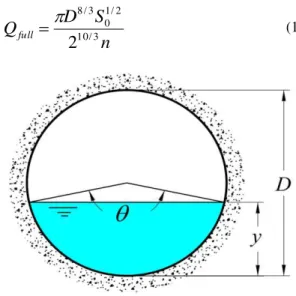
equation for a partially full channel is given by Akgiray (2004):
13/301/2 2/3 5/3 3
/ 8
) sin (
2
n S D
Q (14)
where Q is the ‘true’ discharge and is the water surface angle (Figure 1). In this respect, the corresponding flow area and water surface angle are given by:
) sin ( 8
2
D
A (15)
) 2 1 ( cos
2 1
(16)
where is equal to y/D and y is the flow depth. In a circular channel under full flow conditions (i.e. = 2), Eq. (14) reduces to:
n S D
Qfull 10/3
2 / 1 0 3 / 8
2
(17)
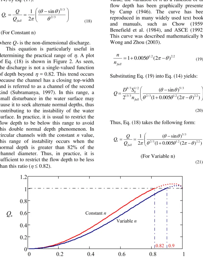
99 Eq. (18) is obtained from dividing Eq. (14) by Eq. (17).
2/3
3 / 5
) sin ( 2
1
full Q
Q Q
(For Constant n)
(18)
where Q* is the non-dimensional discharge. This equation is particularly useful in determining the practical range of . A plot of Eq. (18) is shown in Figure 2. As seen, the discharge is not a single-valued function of depth beyond = 0.82. This trend occurs because the channel has a closing top-width and is referred to as a channel of the second kind (Subramanya, 1997). In this range, a small disturbance in the water surface may cause it to seek alternate normal depths, thus contributing to the instability of the water surface. In practice, it is usual to restrict the flow depth to be below this range to avoid this double normal depth phenomenon. In circular channels with the constant n value, this range of instability occurs when the normal depth is greater than 82% of the channel diameter. Thus, in practice, it is sufficient to restrict the flow depth to be less than this ratio ( 0.82).
In circular channels with the variable n value, the variation of n as a function of the flow depth has been graphically presented by Camp (1946). The curve has been reproduced in many widely used text books and manuals, such as Chow (1959), Benefield et al. (1984), and ASCE (1992). This curve was described mathematically by Wong and Zhou (2003).
2 . 2 2
.
1 (2 )
005 . 0
1
full n
n
(19)
Substituting Eq. (19) into Eq. (14) yields:
) ) 2 ( 005 . 0 1 (
) sin (
2 2/3 1.2 2.2
3 / 5
3 / 13
2 / 1 0 3 / 8
full n S D Q
(20)
Thus, Eq. (18) takes the following form:
) ) 2 ( 005 . 0 1 (
) sin ( 2
1
2 . 2 2
. 1 3
/ 2
3 / 5
full
Q Q Q
(For Variable n)
(21)
100 Based on Eq. (21), the double normal depth phenomenon occurs when is greater than 0.9, as shown in Figure 2. Thus, the practical range in this case is
0.9.
It should be noted that, in computer simulations, it is not necessary to compute the flow depth in very small water depths. Therefore, the minimum value of the dimensionless flow depth is considered as
= 0.1.
Improved Kinematic Wave Parameters (In the Case of Constant n)
Using the implicit differentiation of Q with respect to A, in Eq. (11) can be written as:
/ / A Q Q
A
(22)
Substituting the partial derivatives of Eqs. (14) and (15) into Eq. (22), then
) ) 2 / ( sin
sin 2
. 0 1 ( 3 5
2
(23)
As seen, is a function of (or flow depth) and constant should be determined for a reference depth or angle. The reference coefficient, , is used in lieu of to derive independently of the flow depth. It should be noted that is not dependent on the flow depth while is. Setting = in Eq. (23), then:
) ) 2 / ( sin
sin 2
. 0 1 ( 3 5
2
(24)
By setting this reference value = in Eq. (14), in Eq. (13) becomes
13/33 10/2 2/3 5/3 2
3 / 8
) sin (
2
n S D
(25)
In Eqs. (24) and (25), and are the fitting coefficients. Substituting from Eq. (25) into Eq. (2), the approximate discharge, Qa , can be written as:
( sin ) ( sin )
2 2/3
3 / 5
3 / 13
2 / 1 0 3 / 8
n S D Qa
(26)
Eq. (26) is considered as an ‘approximate’ discharge (power-law) equation. The ‘true’ discharge Q is given by Eq. (14).
Dividing Eq. (26) by Eq. (17), then
) sin ( ) sin (
2 2/3
3 / 5
*
full a a
Q Q Q
(27)
Now, the optimal values of and are determined by minimizing an objective function, z, such that,
2
* ) (
Q Q Q Max z
Minimize a (28)
where the minimization procedure is performed over the practical range of flow depth (0.1 0.82). In this range, the optimal values of the fitting coefficients were found to be = 2.73 rad (or = 0.398) and = 0.96. Substituting these values into Eqs. (24) and (25), the proposed kinematic wave parameters in circular channels with the constant n value are obtained:
370 . 1
101 073 . 0 2 / 1 0 540 . 0 nD S
(For Constant n, 0.1 0.82)
(30) Thus, 37 . 1 073 . 0 2 / 1 0 540 . 0 A nD S Qa
(For Constant n, 0.1 0.82)
(31)
Improved Kinematic Wave Parameters (In the Case of Variable n)
Using Eq. (22) and differentiating Eq. (20) with respect to A, is expressed as:
10000 ) 2 ( 50 ) 2 )( 36 51 ( 5 1 ) 2 / ( sin sin 3 5 3 5 5 / 11 5 / 6 5 / 6 5 / 1 2 (32)
Considering is equal to in Eq. (32).
10000 ) 2 ( 50 ) 2 )( 36 51 ( 5 1 ) 2 / ( sin sin 3 5 3 5 5 / 11 5 / 6 5 / 6 5 / 1 2 (33)
Similarly, considering is equal to in Eq. (20) and using Eq. (13), then:
) ) 2 ( 005 . 0 1 ( ) sin ( 2 2 . 2 2 . 1 3 / 2 3 / 5 3 3 / 13 2 / 1 0 2 3 / 8 full n S D (34)
Substituting from Eq. (34) into Eq. (2), then: ) sin ( ) ) 2 ( 005 . 0 1 ( ) sin ( 2 2 . 2 2 . 1 3 / 2 3 / 5 3 / 13 2 / 1 0 3 / 8 full a n S D Q (35)
In Eqs. (34) and (35), is calculated using Eq. (33). The ‘true’ discharge is given by Eq. (20).
The approximate non-dimensional discharge takes the following form:
) sin ( ) ) 2 ( 005 . 0 1 ( ) sin ( 2 2 . 2 2 . 1 3 / 2 3 / 5 full a a Q Q Q (36)
Now, the optimal values of and can be determined for the practical range of 0.1 0.9, as previously explained. In this case, the optimal values occur at
= 2.45 rad ( = 0.331) and =1.025. Substituting these values into Eqs. (33) and (34), the proposed kinematic wave parameters in circular channels with the variable n value are obtained as:
407 . 1
(For Variable n, 0.1 0.9) (37)
147 . 0 2 / 1 0 470 . 0 D n S full
(For Variable n, 0.1 0.9)
(38) 407 . 1 147 . 0 2 / 1 0 470 . 0 A D n S Q full a
(For Variable n, 0.1 0.9)
102
VERIFICATION OF PROPOSED METHOD
The proposed method was verified using another approximate method for determining the kinematic wave parameters. This method, called effective sensitivity indicator, can be derived using Eq. (11) as follows (Vatankhah et al., 2008):
A Q A
A Q Q
ln ln /
/
(40)
This equation can be written in the following finite difference form:
) / ln(
) / ln( ln
ln
1 2
1 2
A A
Q Q A
Q
(41)
where the subscript ‘1’ and ‘2’ refer to the low and high flow conditions (limits of the most probable operation depth range),
. Then, is given by Eq. (12). The derivation of the kinematic wave parameters for the constant and variable n values using this approximate method is presented in Appendix.
In the case of the constant n value, applying the parameter equations of the Appendix for the range of between 0.1 and 0.82 ( = 0.1 and = 0.82), is calculated as 1.370. The coefficient of in Eq. (30) is calculated as its average value for the preceding two points as 0.519, compared with 0.540. If one more point ( = 0.46) is used, the three points will result in a coefficient equal to 0.534. As seen, a more accurate value of the coefficient can be obtained using more points. In the case of the variable n value, the application of the parameter equations, as described in the Appendix, within the range of between 0.1 and 0.9 ( = 0.1 and = 0.9), is estimated to be 1.407. The approximate coefficient of is similarly calculated using
two and three points and the corresponding values are 0.475 and 0.472, respectively. These values are well matched with the value of 0.470 obtained using Eq. (38). Clearly, the results of the effective sensitivity method, verifies those of the proposed method.
COMPARISON OF ESTIMATED PARAMTERS WITH EXISTING METHOD
Estimated Discharge Comparison
The accuracy of the proposed kinematic parameter equations using the accurate point-sensitivity indicator method is compared with the one proposed by Wong and Zhou (2003). The error in estimating the discharge is defined as:
Q Q
e(%) 100 1 a
(42)
The true discharge, Q, is given by Eq. (14) for the constant n value and by Eq. (20) for the variable n value. The approximate discharge, Qa, using the proposed method is given by Eq. (31) for the constant n value and by Eq. (39) for the variable n value. In the method of Wong and Zhou (2003) (WZ), Qa is calculated by substituting kinematic wave parameters of Eqs. (7) and (8) into Eq. (2) for the constant n value and the parameters of Eqs. (9) and (10) into Eq. (2) for the variable n value.
103 Thus, estimates obtained using the proposed method are generally conservative. In the case of the variable n value, the comparison between the results is shown in Figure 4. As seen, the error of the proposed method ranges from –1.4% to 1.4%, while the error associated with the WZ method ranges from –0.4% to 6%.
Fig. 3. Comparison of the errors in the estimated discharge of proposed and existing kinematic
parameters for constant n value.
Fig. 4. Comparison of the errors in the estimated discharge of proposed and existing kinematic
parameters for variable n value.
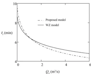
Travel Time Comparison
The travel time, tt, in a channelis given by (Wong and Zhou, 2003):
u d
u d
t
Q Q
Q Q
L t
/ 1 / 1
/
1 (43)
where L is the length of the channel segment, Qu is the upstream inflow, and Qd is the downstream outflow of the channel segment. The inflow and downstream outflow are related together by:
Qd = Qu + Lq (44)
where q is the uniform lateral inflow.
Fig. 5. Comparison of the travel time of proposed and existing methods for constant n value.
104
CONCLUDING REMARKS
This paper presented improved equations for estimating the kinematic wave parameters using two types of sensitivity indicators. Based on the results of this study, the following comments are offered:
1. The kinematic wave parameters were mathematically obtained for circular cross sections in two different cases with constant and variable Manning’s roughness coefficients. In the case of the constant n value, the new estimated parameters were more accurate than the existing parameters. In the case with the variable n value, the estimated parameters using the proposed method yielded more accurate parameters than the parameters obtained using the existing method. Therefore, the new proposed method is recommended to estimate the parameters for the implementation in practice.
2. The point-sensitivity method was used to develop depth-independent kinematic wave parameters. This method, which adopts optimization, produced accurate parameters that are applicable to the full practical range of flow depth. These parameters are useful when specific information about flow depth is not available or not reliable. The results showed that the error associated with estimating the discharge was less than 4% in the case of the constant n value, compared to up to 40% when the existing method was used.
3. The proposed (point-sensitivity) method for estimating kinematic wave parameters was verified using another method based on effective sensitivity. This method is approximate, but simple, and can be used to produce kinematic wave parameters for system-specific conditions, such as a desired range of flow depth especially when such a range is small. In fact, in such conditions, the effective-sensitivity method would be
preferable as it would produce local, perhaps more relevant parameters.
4. The travel time in circular channels, which is an essential element in drainage design, is a function of the kinematic wave parameters. The kinematic wave parameters presented in this paper can be used to accurately estimate the travel time in circular channels.
5. This study showed that the kinematic wave celerity concept is a powerful tool to estimate kinematic wave parameters. This approach can be also applied to other cross sections for which the kinematic wave parameters cannot be expressed mathematically independent of the flow depth, such as trapezoidal, rectangular, parabolic, and power-law. The method is not likely to be applicable to compound channels. This research area is currently being explored by the authors.
APPENDIX
Effective Sensitivity Method for Kinematic Parameter Estimation
For the Manning's formula with constant n, Eq. (41) is written as:
) / ln(
) / ln( 3 2 3 5
1 2
1 2
A A
P P
(A1)
which for a circular channel reduces to:
)] sin /(
) sin ln[(
) / ln( 3
2 3 5
1 1
2 2
1 2
(A2)
Also using Eq. (12) one obtains:
13/33 01/2 2/3 5/3 2
3 / 8
) sin (
2
n S D
105 Then, an approximate coefficient of Eq. (A3) is calculated as the average at three
different values of as
[ () + [() / 2] + ()] / 3.
For Manning formula with variable n value, Eq. (41) is written as:
) / ln( )] / ( ) / ln[( 3 5 1 2 1 2 3 / 2 1 2 A A n n P P (A4)
For a circular channel, Eq. (A4) is:
1 1 2 2 2 . 2 1 2 . 1 1 2 . 2 2 2 . 1 2 1 2 sin sin ln ) 2 ( 005 . 0 1 ) 2 ( 005 . 0 1 ln ln 3 2 3 5 (A5)
Also using Eq. (12) one obtains:
) ) 2 ( 005 . 0 1 ( ) sin ( 2 2 . 2 2 . 1 3 / 2 3 / 5 3 3 / 13 2 / 1 0 2 3 / 8 full n S D (A6)
Then, the approximate coefficient of is calculated as previously described.
NOTATION
A = flow area,
D = diameter of the circular channel, e = percentage error of discharge, L = length of the channel segment, n = Manning's roughness coefficient, nfull = Manning's roughness coefficient under the full flow condition,
P = wetted perimeter, Q = discharge,
Q = lateral inflow,
Qa = approximate discharge,
Qfull = discharge in channel under full flow condition,
Qt = true discharge, Qu = upstream inflow, R = hydraulic radius
S0 = bed slope of the channel, T = time,
Tt = time of travel, x = distance, y = flow depth,
= water surface angle,
= relative flow depth y/D,
= a fitting value,
and = kinematic wave parameters,
= channel surface roughness,
= kinematic viscosity.
REFERENCES
Akgiray, O. (2004). “Simple formulae for velocity, depth of flow, and slope calculations in partially filled circular pipes”, Environmental Engineering
Science, 21(3), 371-385.
American Society of Civil Engineers and Water Environment Federation (1992). “Design and construction of urban stormwater management systems”, ASCE Manual and Reports of
Engineering Practice, No. 77. New York, N.Y.
Benefield, L.D., Judkins, J.F. and Paar, A.D. (1984). “Treatment plant hydraulics for environmental engineers”, Prentice-Hall, Englewood Cliffs, N.J. Camp, T.R. (1946). “Design of sewers to facilitate
flow”, Sewage Works Journal, 18(1), 3-16.
Chow, V.T. (1959). “Open channel hydraulics”, McGraw-Hill, New York.
Chow, V.T., Maidment, D. and Mays, L.W. (1988). “Applied hydrology”, McGraw-Hill, New York. Christensen, B.A. (1984). “Discussion of Flow
velocities in pipelines”, Journal of Hydraulic
Engineering, 110(10), 1510–1512.
Hager, W.H. (1989). “Discussion of Noncircular sewer”, Journal of Environmental Engineering,
115(1), 274–276.
Haltas, I. and Kavvas, M.L. (2009). “Modeling the kinematic wave parameters with regression methods”, Journal of Hydrological Engineering,
14(10), 1049-1058.
106
dynamics”, Report No. 133. Ralph M. Parsons Laboratory for Water Resources and Hydrodynamics, Massachusetts Institute of Technology, Cambridge, MA.
Jain, S.C. (2001). Open channel flow, John Wiley and Sons, New York.
Lighthill, M.J. and Whitham, C.B. (1955). “On kinematic waves: Flood movement in long rivers”, Proceedings of Royal Society (London), Series A, 229, 281-316.
MacArthur, R.C. and DeVries, J.J. (1993). “Introduction and application of kinematic wave routing techniques using HEC-1”, Training Document 10, U.S. Army Corps of Engineers. Subramanya, K. (1997). “Flow in open channels”,
Tata McGraw-Hill, New Delhi.
Vatankhah, A., Kouchakzadeh, S. and Hoorfar, A. (2008). “Developing effective sensitivity indicator for irrigation network components”, International
Journal of Applied Agricultural Research, 3(1)
17-36.
Wong, T.S.W. and Zhou M.C. (2006). “Kinematic wave parameters for trapezoidal and rectangular channels”, Journal of Hydrologic Engineering,
11(2), 173-183.
Wong, T.S.W. and Zhou, M.C. (2003) “Kinematic wave parameters and time of travel in circular channel revisited”, Advances in Water Resources,