How to measure market liquidity risk in financial institutions?

(1)

Department of Political Economy

How to Measure Market Liquidity Risk in Financial Institutions?

Joana Maria Cabrita Lopes

A Dissertation presented in partial fulfillment of the Requirements for the Degree of

Master

Supervisor:

Dr. João Pedro Pereira, Assistant Professor, ISCTE Business School – Lisbon University Institute

Co-supervisor:

Dr. Umut Çetin, Lecturer in Statistics,

Department of Statistics – London School of Economics and Political Science

(2)

II

“Liquidity always comes first; without it, a bank doesn't open its doors;

with it, a bank may have time to solve its basic problems.”

(3)

III

Summary

We apply numerical stochastic dynamic programming to derive trading strategies that minimize the mean and variance of the costs of executing a large block of a security over a fixed exogenously defined time period. Financial markets are considered to be liquid if a large quantity can be traded quickly and with minimal price impact. Although, the trading costs associated with trading such large quantity of a single asset – often called execution or transaction costs – can be substantial significant that directly influence the return of the investment. To minimize the price impact, an investor would choose to split his order into many small pieces. However the time taken to transact introduces a risk component in execution costs that arise from unfavourable price movements during the execution of an order. The longer the trade duration, the higher the uncertainty of the realized prices. In this setting, the decision can be viewed as a risk/reward trade-off faced by the investor who not only cares about the expected value but also about the variance (or volatility) of his execution costs. Risk aversion in this context means that an investor is willing to trade lower risk for higher price impact costs. A numerical solution for minimizing a combination of the expected transaction costs and volatility (or price) risk is derived. The parameters of the price impact model are estimated based on real world stock data.

Keywords: market liquidity risk; transaction costs; optimal trading strategies; stochastic

dynamic programming.

(4)

IV

Resumo

A globalização e o desenvolvimento dos mercados financeiros nos últimos anos implicaram uma crescente dependência das instituições financeiras do financiamento nos mercados internacionais, com a utilização de instrumentos financeiros cada vez mais complexos, criando assim novos desafios na gestão do risco de liquidez. Este desenvolvimento dos mercados e a recente crise de 2008 realçaram a importância vital de existir um adequado sistema de mensuração do risco de liquidez para uma melhor eficácia no funcionamento do sector bancário.

No período que antecedeu a crise do subprime, os mercados estavam confiantes e o financiamento estava facilmente acessível e a baixo custo. A alteração das condições de mercado ilustraram quão rapidamente a liquidez se pode evaporar e repercutir-se durante um longo período.

O caso LTCM (Long Term Capital Management) tem um especial interesse para a gestão do risco de liquidez uma vez que as posições detidas pelo fundo revelaram ser demasiado elevadas para serem liquidadas sem induzir grandes movimentos nos preços de mercado devido à insuficiente liquidez do mesmo. A escassez repentina de liquidez nos mercados é um sintoma observado na maioria das crises financeiras. Assim, a identificação, quantificação, monitorização e controlo do risco de liquidez assumem um papel de destaque quer para as instituições financeiras quer para os reguladores.

Os modelos usados na quantificação do risco de mercado, tipicamente Value at Risk

models, geralmente não consideram se o preço de mercado de um determinado título (ou

carteira de títulos) pode ou não ser realizado em caso de liquidação, ou seja não consideram o risco de liquidez de mercado. Esta situação pode conduzir a uma sub-estimação do risco total e consequentemente a uma errada alocação de capital.

Neste sentido, esta dissertação pretende responder à questão: Como medir o risco de liquidez (de mercado) nas instituições financeiras?

Podemos distinguir dois principais tipos de risco de liquidez: o risco de liquidez de financiamento e o risco de liquidez de mercado, existindo uma forte relação entre ambos. O risco de liquidez de financiamento é o risco de um banco não poder honrar os

(5)

V seus compromissos financeiros nas datas devidas sem incorrer em perdas significativas. A consequente necessidade de financiamento pode requerer a venda de activos podendo afectar a liquidez de mercado. O risco de liquidez de mercado é o risco de uma posição não poder ser facilmente liquidada (e num curto espaço de tempo) sem influenciar substancialmente o preço de mercado.

Apesar da ligação entre os dois tipos de risco, estes são objecto de estudo de áreas distintas da economia e finanças. O primeiro é estudado no âmbito da Gestão de Activos e Passivos (ALM) e o segundo, o risco de liquidez de mercado, é um tópico da micro-estrutura dos mercados e das estratégias óptimas de negociação.

As estratégias óptimas de negociação dizem respeito à gestão e mensuração dos custos associados à transacção de títulos e à definição de estratégias que minimizam esses custos. Assim, medir o risco de liquidez de mercado implica medir os custos de negociação, que, embora incertos, dependem do impacto no preço o qual é influenciado pelo volume transaccionado. O risco de liquidez de mercado, e consequentemente as estratégias óptimas de negociação, serão o tema central desta dissertação.

Um problema típico enfrentado pelas instituições financeiras (e pelos grandes investidores, e.g., os investidores institucionais) é a liquidação (ou aquisição) de grandes posições num determinado activo, tal como um grande volume de acções. Considera-se que os mercados financeiros são líquidos quando uma grande quantidade pode ser transaccionada rapidamente e com um impacto mínimo no preço. No entanto, a execução imediata frequentemente não é possível ou apenas é a um custo demasiado elevado devido à reduzida liquidez do mercado.

O impacto no preço e os custos de execução (também denominados de custos de transacção ou de negociação) podem ser significativamente reduzidos dividindo a ordem (de venda ou de compra) em ordens mais pequenas repartidas por um determinado horizonte temporal. Assim, uma questão pertinente é: como definir estratégias óptimas de negociação de modo a que os custos esperados de execução sejam minimizados? Problemas deste tipo têm sido objecto de estudo de vários autores, entre os quais se destacam Bertsimas and Lo (1998).

Contudo, o tempo total necessário para executar uma grande quantidade introduz uma componente de risco nos custos de execução que resulta dos movimentos não favoráveis

(6)

VI no preço que podem ocorrer durante o período de execução. Quanto maior o tempo de execução maior será a incerteza dos preços realizados. Os investidores avessos ao risco negociarão mais rápido, incorrendo em custos de transacção mais elevados mas com menor risco. Neste sentido, a decisão pode ser encarada como um custo/beneficio do investidor que tem em conta não somente o valor esperado dos custos mas também a variância dos mesmos.

Assim, considerando apenas o custo esperado de execução como „função objectivo‟ deixa de parte uma importante componente da liquidez que é o risco de volatilidade que está associado ao prolongar (a venda ou compra) de uma transacção. Por este motivo, Almgren and Chriss (2000) sugeriram substituir a minimização dos custos esperados pela minimização do valor esperado e da variância dos custos resolvendo o respectivo problema de optimização na classe das estratégias determinísticas (ou estáticas).

No entanto, o simples acto de negociar afecta não só os preços actuais mas também a dinâmica de preços, que por sua vez, afecta os custos de negociação futuros. Assim, medir os custos de transacção é um problema fundamentalmente dinâmico e não estático.

Por consequência, estudou-se o modelo dinâmico de Bertsimas and Lo alterando a „função objectivo‟ de modo a incorporar o risco de volatilidade (ou risco de preço). Em vez de se minimizar apenas os custos esperados de executar um grande volume de acções durante um período finito de tempo (exogenamente definido) derivou-se uma estratégia óptima de negociação que minimiza uma combinação entre os custos de transacção e o risco. Este problema de optimização pode ser resolvido recorrendo à programação dinâmica estocástica e resolvido numericamente à luz da equação de Bellman (1957). Sendo um problema recursivo o algoritmo utilizado foi o algoritmo de indução inversa, ou seja, indução do futuro para o presente (backward induction), uma vez que no último período o número de acções a negociar é conhecido (são as que restam).

No modelo de Bertsimas and Lo o preço de execução é composto por duas componentes, uma componente sem impacto no preço, que resulta da evolução normal do preço na ausência de impacto (pode ser medida pelo ponto médio entre o preço de compra e venda), e uma componente denominada „impacto no preço‟ que é uma função

(7)

VII linear do volume negociado e das condições de mercado (e informação disponível). Os parâmetros do modelo foram estimados com base em dados históricos de bolsa. Na estimação dos parâmetros da componente „impacto no preço‟ utilizou-se uma regressão linear.

Com base no algoritmo de optimização, desenvolvido em linguagem MATLAB, fez-se uma análise comparativa entre a estratégia óptima de negociação que considera a componente da volatilidade (ou risco) e a que não considera, para diversos valores dos parâmetros. Com base nos resultados as principais conclusões foram as seguintes:

 O risco (caracterizado por uma função objectivo quadrática) é uma componente importante dos custos de transacção que não deve ser ignorada;

 Os custos de execução aumentam com a quantidade transaccionada, ou seja, quanto maior for o volume transaccionado maior será o impacto no preço e consequentemente maiores serão os custos de transacção;

 Quando o peso da informação disponível aumenta os custos de transacção diminuem, uma vez que o acesso à informação e às condições de mercado implicam um conhecimento da tendência dos preços de mercado podendo o investidor tirar partido dessa informação;

 Existem evidências que levam a concluir que o aumento da volatilidade do título negociado aumenta os custos de transacção;

 Quanto maior o tempo total da transacção menor serão os custos de execução, dado que a quantidade transaccionada vai diminuindo;

 Os investidores mais avessos ao risco assumem maiores custos de transacção de modo a reduzirem a sua exposição ao risco.

(8)

VIII

Acknowledgements

Firstly, I would like to thank Professor João Pedro Pereira for his availability, awareness and background, and for his valuable comments.

As well, I would like to express my gratitude to Professor Umut Çetin for his thoughts and for giving me the opportunity to live an unforgettable experience at the London School of Economics and Political Science.

To Pedro for always believing in me and for his encouraging words in the troubling moments.

And last but not least to my sister Margarida and to my parents Esilda and José for their unconditional support.

(9)

IX

List of Tables

Table 1 – Characteristics of a Dynamic Programming... 19

Table 2 – Security information ... 31

Table 3 – Estimated drift and volatility of no impact price ... 34

Table 4 – Regression output ... 35

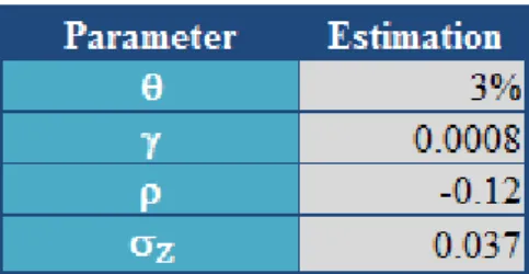
Table 5 – Estimated parameters of the linear-percentage temporary price impact model ... 37

Table 6 – Estimated execution costs (in cents per share) for the optimal execution strategy and for the naïve strategy for different values of the price impact parameter  38 Table 7 – Estimated execution costs (in cents per share) for the optimal execution strategy and for the naïve strategy for different values of the price impact parameter  39 Table 8 – Estimated execution costs (in cents per share) for the optimal execution strategy and for the naïve strategy for different values of the price impact parameter  39 Table 9 – Estimated execution costs (in cents per share) for the optimal execution strategy and for the naïve strategy for different values of the daily standard deviation Z ... 40

Table 10 – Estimated execution costs (in cents per share) for the optimal execution strategy and for the naïve strategy for different values of the number of periods T (in days) ... 40 Table 11 – Estimated execution costs (in cents per share) for the optimal execution strategy and for the naïve strategy for different values of the risk aversion parameter λ41

(12)

XII

List of Figures

Figure 1 – Effect of position size on security price ... 9 Figure 2 – Permanent and temporary price impact from sale... 13 Figure 3 – Different execution strategies ... 15 Figure 4 – Last price (in LTL) of Ukio Bankas Security from January to December 2009 ... 32 Figure 5 – Close price (in USD) of S&P500 Index from January to December 2009 ... 32 Figure 6 – Mid price of Ukio Bankas Security from January to December 2009 ... 33 Figure 7 – Mid price log returns of Ukio Bankas Security from January to December 2009 ... 33 Figure 8 – Log returns of S&P500 Index from January to December 2009 ... 34 Figure 9 – Value function of the naïve strategy for T=20 and S=10 (considering the estimated parameters) ... 52 Figure 10 – Value function of the optimal strategy for T=20 and S=10 (considering the estimated parameters) ... 53

(13)

XIII

List of Abbreviations

ALM BLUE DP DW EC EWMA HJB IID LPT LTCM LTL LVaR MTM OLS PDF USD VaR WN

Asset and Liability Management Best Linear Unbiased Estimator Dynamic Programming

Durbin Watson (Test) Execution Costs

Exponentially Weighted Moving Average Hamilton-Jacobi-Bellman (Equation) Independently and Identically Distributed Linear-Percentage Temporary

Long Term Capital Management Lithuanian Litas

Liquidity-adjusted Value at Risk Mark-To-Market

Ordinary Least Squares Probability Density Function United States Dollar

Value at Risk White Noise

(14)

1

Chapter 1 Introduction

Financial market developments in the last years, such as the increasing reliance of large institutions on market funding, the increasing use of complex financial instruments, and the globalisation of financial markets, have created significant new challenges in liquidity risk management1. These market developments, and the 2007-2008 market turmoil, highlight the vital importance for the soundness of the banking sector to have adequate liquidity risk measurement systems for both normal and stressed times, and to maintain adequate liquidity buffers.

Prior to the turmoil, markets were confidant and funding was readily available at low cost. The change in market conditions illustrated how quickly liquidity2 can evaporate and that illiquidity can last for an extensive period of time.

The case of Long Term Capital Management (LTCM) is also of special interest for liquidity risk management because positions held by the fund were too large to be liquidated without inducing major price movements due to insufficient market liquidity. Commonly, the sudden dry up of market liquidity is a symptom observed in most of financial market crises.

The Value at Risk (VaR) models, often used for the estimation of market risk, generally do not consider whether the market price of a security can actually be realized in case of a liquidation. This may lead to an underestimation of the total risk, and hence to a misleading capital allocation.

1_{The fundamental role of banks in transforming short-term deposits into long-term loans makes banks} inherently vulnerable to liquidity risk. Liquidity risk management is the constant process of balancing the cash inflows and outflows from on- and off-balance sheet items, along with structural and strategic planning, to ensure both that adequate sources of funding are available, and that those sources are used properly. Liquidity risk management also requires robust internal governance, adequate tools to identify, measure, monitor, and control liquidity risk, including stress tests and contingency funding plans.

2

(15)

2 Therefore, this dissertation aims to answer the question: How to measure (market) liquidity risk in financial institutions?

One can distinguish two main types of liquidity risk, funding liquidity risk and market liquidity risk3. Funding liquidity risk is the risk that a bank will not be able to honour its financial commitments when they are due without incurring substantial loss. Market liquidity risk is the risk that a position cannot easily be liquidated without significantly influencing the market price.

A typical problem faced by financial institutions is the liquidation (or acquisition) of a large asset position, such as a large block of shares. An immediate execution is often not possible or only at a very high cost due to a scarce liquidity of the market.

The overall price impact and the execution costs (also called „transaction costs‟) can be significantly reduced by splitting the order into a sequence of smaller orders that are spread over a certain time horizon. Hence, one pertinent issue is to find optimal trading strategies such that the expected execution costs are minimized. Problems of this type were analyzed by many authors, namely Bertsimas and Lo (1998).

Nevertheless, the time taken to transact introduces a risk component in execution costs. Risk averse agents will trade more rapidly thus incurring higher transaction costs but lower risk. Consequently, taking the expected execution costs as a target function misses an important component of liquidity, the volatility risk that is associated with delaying an order. For that reason, Almgren and Chriss (2000) suggested replacing the minimization of expected costs by a mean-variance optimization of costs solving the correspondent optimization problem in the class of deterministic (or static) strategies. Although measure executions costs is a dynamic (stochastic) problem, not static, since trading transactions affects both current and future prices.

We therefore propose to study the „linear-percentage temporary‟ dynamic model of Bertsimas and Lo by changing the objective function in order to incorporate the volatility risk component (or price risk). Instead of minimizing merely the expected transaction costs of trading a large block of equities over a (fixed) finite horizon we derive a dynamic optimal trading strategy that minimizes a combination of trading costs

3

Furthermore, in literature, we can find another liquidity risk types, such as: call liquidity risk, term liquidity risk and contingent liquidity risk. For more detail please see Appendix A.

(16)

3 and volatility (or price) risk. It can be seen as a typical problem of stochastic dynamic programming and can be solved numerically based on the „Bellman‟s Equation‟.

This dissertation is organized as follows: Chapter 2 introduces some concepts related with market liquidity risk and his components; Chapter 3 discusses optimal trading strategies. In Chapter 4 we review dynamic programming theory. Chapter 5 explicitly examines the linear percentage temporary model and Chapter 6 presents and discusses numerical results based on real data. Last chapter concludes.

(17)

4

Chapter 2 Market Liquidity

Asset returns are usually calculated using mid market or closing prices. Typical measures of market risk are based on these returns. Implicitly, it is assumed that these are the prices that can be achieved in case of liquidation. This is the point, where (market) liquidity risk comes into play. Market liquidity risk deals with the risk of losses arising from the deviation of the realised price in a buying/selling process as compared to the market price prevailing prior to the transaction. This loss is denoted as the transaction cost, representing an additional charge when buying, and taking the form of a price discount when selling an asset. The relevant market price is the mid-price between bid and ask as the best available estimate of the fair value of the security. By taking the mid-price, trading cost is split equally between buy and sell transactions.

2.1 Market Liquidity and Funding Liquidity: Definition and

Interactions

Funding (or cash flow) liquidity risk is the risk that a bank will not be able to honour its financial commitments (both expected and unexpected current and future cash flows) when they are due without incurring substantial loss. The consequent need for cash may require selling assets. Market (or asset) liquidity risk is the risk that a position cannot easily be liquidated at short notice without significantly influencing the market price, because of inadequate market depth or market disruption, and hence the liquidation value of the position will differ significantly from their current mark-to-market (MTM) value4. Thus liquidity risk can arise from both, the assets and liabilities of a financial institution.

4

Mark-to-market value refers to accounting for the value of an asset or liability based on the current market price of the asset or liability.

(18)

5 The increasing market-based funding of banks originate a correlation between funding liquidity risk and market liquidity risk since market illiquidity can difficult a bank to raise funds by selling assets and thus increase the need for funding liquidity. The resulting changes in demand for funds can, afterwards, affect market liquidity.

Despite the relation between market and funding liquidity, usually they are treated in two distinct branches of economics and finance.

Funding liquidity risk results from size and maturity mismatches of assets and liabilities which is subject of Asset and Liability Management (ALM), while market liquidity risk is a topic of market microstructure theory and optimal trading strategies. Therefore, concepts for measuring and managing the two types of liquidity differ substantially from each other.

Assessing funding liquidity risk implies checking the asset and liability structure of a financial institution and the potential demands on cash and other sources of liquidity. Asset and Liability Management unit is in charge of managing the differences, at all future dates, between assets and liabilities of the banking portfolio. Controlling (funding) liquidity risk implies controlling over time the cash flows, avoiding unexpected market funding and maintaining a „cushion‟ of liquid (short-term) assets5, so that selling them provides liquidity without incurring in losses. Liquidity risk exists when there are deficits of those funds. When there are excess of funds the result is interest rate risk, the risk of not knowing in advance the rate of lending or investing these funds.

Market microstructure theory studies the role of trading mechanisms on the price setting process. This area of literature examines the ways in which the market structure and trading mechanisms, i.e., the evolution process of a market, affects transactions costs, prices, volume and trading behaviour. Optimal trading strategies concerns with the measurement and management of trading costs and the definition of strategies that minimize those costs. Therefore, measuring market liquidity risk implies measure

5_{Liquid assets are usually defined as assets that can be quickly and easily converted into cash in the} market at a reasonable cost.

(19)

6 transaction costs which are uncertain and a function of the price impact of trades and the size of the positions. Market liquidity risk (and optimal trading strategies) constitutes the main focus of this dissertation and will be treated in depth in subsequent sections.

2.2 Trading Costs Components

Trading costs, also called execution or transaction costs, have several components: specific costs such as commissions and bid-ask spreads, and costs that are harder to quantify, such as the opportunity cost of waiting and the price impact from trading. Opportunity costs arise because market prices are moving constantly and can change favourably or unfavourably, generating unexpected profits or lost opportunities while a trader hesitates.

Glantz and Kissell (2003) identify nine components of trading costs: broker commissions, exchange fees, taxes, bid-ask spreads, investment delay, price appreciation, price impact, timing risk and opportunity cost.

2.3 Market Liquidity Measures

Liquidity risk is one of the factors, typically ignored in Value at Risk estimates, which is a widely used measure of market risk. It is assumed that any portfolio position is liquidated in a single block and the mark-to-market value is always fully realised. Since the postulate of infinitely elastic markets contradicts the premise of prudence in risk management, some ad-hoc adjustments to VaR have been proposed. Time horizon and volatility are the two parameters through which the VaR number can be changed in order to account for an increase in liquidity risk. Often, the time adjustment is implemented for all portfolio positions as a ten day holding period which is required by regulatory authorities. Increasing the time horizon over which VaR is calculated (frequently through the “square root of time” rule) to account for the time taken to liquidate a large position, from an economic perspective, this procedure has severe limitations, as capital would be tied up inefficiently if positions can be sold quicker than the assumed minimum holding period. In addition, the “square root of time” rule,

(20)

7 assumes that no autocorrelation exists between returns from one measurement period to another. Another possibility to take liquidity risk into account is to multiply the VaR measure by some conservative factor. Nevertheless, all above mentioned approaches leave the question of how much and by what criteria the VaR measure should be altered or not. As so, a liquidity risk measure should be based on quantitative, measurable criteria.

2.3.1 Bid-Ask Spreads

One of the components of transaction costs and most popular measure of liquidity is the bid-ask spread. Lower transaction costs and hence a narrower spread reflects a better liquidity in the market. The absolute bid-ask spread is simply defined as the difference between the (best) ask price (lowest price for which a seller is willing to sell a security) and the (best) bid price (highest price that a buyer is willing to pay for a security). In relative terms can be calculated by relating the absolute spread to the mid price of the security:

(1)

where _and _{are the bid and ask prices of a security in time t and the mid price} of a security is defined as:

₍₂₎

Relative spreads enhance comparability between the spread sizes of different securities.

Bangia et al. (1999) further split liquidity risk into an exogenous and an endogenous component. Exogenous illiquidity is determined by factors beyond the individual trader‟s control and is equally relevant for all market participants. It describes the part of liquidity cost which is not affected by the size of the position in the market, is the result of market characteristics. Observable variables, such as depth and bid-ask spread, make it measurable. In contrast, endogenous liquidity risk is specific to the position in the market and varies across market participants. It is mainly driven by the size of a position held: the larger the size of the position, the greater is the exposure to endogenous liquidity risk. Nevertheless, it can be influenced by the trader‟s own actions by applying appropriate trading schedules like splitting a large order into smaller pieces.

(21)

8 Bangia et al. (1999) only include exogenous liquidity risk in their liquidity adjusted VaR measure considering the uncertainty in the spread. They characterize the distribution of the relative spread by its mean ( ) and standard deviation or volatility ( ). They adjust the VaR measure considering the worst increase in the spread at some confidence level, known as Liquidity-adjusted Value at Risk (LVaR) which combines market and liquidity risk:

₍₃₎

where a is the scaling factor such that (1-α)% percent of liquidation cost is covered. This assumes that the worst market loss and increase in spread will occur at the same time. In general is true, we observe a correlation between returns and spreads.

Although this approach has the merit of considering some transaction costs, it only looks at the bid-ask spread component of this costs, which may be enough for a small position of a stock but is not when liquidation can affect market prices. The price impact factor should be taken into account.

2.3.2 Price Impact

The liquidation price is not only a function of time but also of position size. For positions up to a specific size, usually the current market depth, the transaction can be accomplished at the bid or ask price depending on the direction of the trade. For quantities exceeding market depth, an additional price discount, commonly called price (or market) impact, has to be accounted for. Price impact is the typically unfavourable effect on prices that the process of trading creates: a security‟s seller will, by the very act of selling, push down the security‟s price, and, in the opposite way, a security‟s buyer will, by the very act of purchasing, push up the security‟s price.

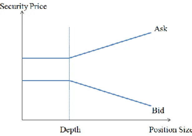
Moreover, the sell/buy price is a decreasing/increasing function of quantity and the larger the order, the more heavily the trade affects the price. However, the functional form that this price-volume relationship takes is not clear. For simplicity, it is often assumed to be linear, whereas there is empirical evidence of concave in case of a buy order as well as convex in case of a sell order. This price-size function is illustrated in

(22)

9 Figure 1, which shows the relationship between the liquidation price and the total position size held.

Figure 1 – Effect of position size on security price

Price impact is an important parameter for the estimation of optimal liquidation strategies, as it can be reduced by slicing the order into several trades. The premium paid for a buy order and the concession made for a sell order can be interpreted as incentives for other market participants to provide additional liquidity. Thus, a large order can be completed within reasonable time.

Bertsimas and Lo (1998) proposes a model which, given a price-impact function, furnishes the optimal sequence of trades that minimizes the expected transaction costs. Nevertheless, their approach ignores the volatility of costs for different trading strategies, i.e., a penalty for the uncertainty of cost (or revenue).

2.3.3 Expected Transaction Costs and Volatility

The drawback of liquidating a large block of a security more slowly, however, is that the portfolio remains exposed to price risk over a longer period. The immediate sale yields to a high cost but minimum risk. Under the uniform sale, the position is sold off in equal size blocks, leading to low cost but higher volatility. Execution strategies do not need to be limited to those two extreme cases – immediate or uniform liquidation. More generally, we can select a strategy that leads to an optimal trade-off between execution costs and price risk.

(23)

10 Almgren and Chriss (2000) examined market liquidity risk by minimising a combination of volatility risk and expected transaction costs arising from (permanent and temporary6) price impact. The rationale is the following: a trading schedule is only optimal if it involves least cost for a certain level of risk and also least risk for a certain level of cost. Such strategies can be determined by minimising the mean-variance objective function for various levels of risk aversion.

They considered the risk-reward trade-off both from the point of view of classic mean-variance optimisation and of VaR. Their analysis led to general insights into optimal trading strategies, and to several applications including a definition of liquidity-adjusted VaR.

2.4 Market Liquidity Features

Market liquidity is usually determined by four key factors:

The tightness of the market, which is measured using the bid-ask spread (as seen before, the difference between buy and sell prices), determines the cost of unwinding a position at short notice. The smaller the difference between the ask and bid prices, the better the liquidity in the market.

The depth of the market assesses which transaction volume can be realised immediately without affecting prices. Small amounts should be able to be traded without impact on prices, for large amounts, a premium for buy orders and a discount for sell orders have to be accepted.

Resiliency describes the speed at which market prices return to equilibrium after a major

transaction.

Immediacy is defined as the time between the start of a market transaction and its final completion. It denotes the speed with which a position is liquidated.

If demand meets supply, even for relatively large trading volumes, and if price impact is minimal, transaction costs are low and the market is considered liquid. A market is

6

The difference between temporary and permanent price impact will be described afterwards in Chapter 3.

(24)

11 perfectly liquid if any volume can be traded at any time at no cost. Since there are no infinitely deep markets, an investor who wishes to trade a large block immediately, as we mentioned before, needs to pay a premium for a buy order or accept a discount for a sell order. These factors increase with the size of the transaction. By splitting the block into smaller orders the investor should be able to reduce transaction costs. The splitting strategies which minimize the transaction costs are known as “optimal liquidation strategies” and would be explained in the subsequently chapter. Another way to minimize transaction costs is to limit the exposure of the security in order to avoid a large price impact in case of forced liquidation.

(25)

12

Chapter 3 Optimal Liquidation Strategies

An optimal trading strategy describes how a large order should be sliced into pieces over a period of time. If a large position is held, the financial institution most likely won‟t liquidate it all at once, but will rather split it up into several orders. This strategy reduces expected transaction costs, implying that liquidation costs and risks will depend on the strategy and the time horizon chosen. Trying to find an optimal trading strategy, not only price impact, but also volatility risk has to be taken into account. During the liquidation period, remaining parts of the holdings are exposed to price risk. An optimal liquidation strategy is the result of a balance between a reduction in potential price impact and an additional exposure to volatility (or price) risk.

The priority objective for the design of such a strategy is to preserve asset value, that is, to minimise the cost component in the presence of risk. In its basic form, the optimization condition only involves price impact as the cost component and price volatility as the only risk factor. A strategy is evaluated according to its expected cost-risk profile: an aggressive strategy, characterised by large initial trades, leads to high price impact cost, but reduces price risk by quickly selling off or buying the remaining shares. Trading more passively, namely shifting parts of the trades to later periods would cause less price impact at the expense of an increase in risk. As price impact costs are a decreasing function of time and the risk of a strategy is increasing over time, it can, as a general rule, be concluded that the change of one term affects the other adversely.

3.1 Temporary and Permanent Price Impact

Some authors distinguish two kinds of price impact: temporary and permanent. Temporary impact refers to temporary imbalances between supply and demand caused by our trading leading to temporary price movements away from equilibrium. Permanent impact means changes in the “equilibrium” price due to our trading, which

(26)

13 remain at least for the life of our liquidation. Figure 2 represents the price movement during the trading period.

Figure 2 – Permanent and temporary price impact from sale

3.1.1 Temporary Price Impact

Temporary price impact arises due to a short-term demand and supply imbalance caused by one‟s own order. When a trader posts a sell order exceeding market depth, he has to accept lower prices in order to complete the trade. If the motives of the trader were purely liquidity-based and other market participants were aware of this motivation, the price would fully recover shortly after the trade hits the market. One of the key questions is how long it takes for the price to return to its pre-trade level. The most common assumption is that temporary price impact will have dissipated completely until the next trade. This implies that in such a model trading intervals cannot be chosen arbitrarily small, as prices need time to return to equilibrium.

The larger the order one wishes to trade in a period, the higher will be the premium the market requires for a buy order (or the concession for a sell). Therefore, temporary price impact in its simplest form is chosen to be an increasing linear function of trading size in a particular period.

Almgren and Chriss (2000), however, state that the true price impact function is probably nonlinear. Hence, in the later papers Almgren (2003) and Almgren (2005) extend the price impact model to accommodate nonlinear functions for temporary price impact.

(27)

14

3.1.2 Permanent Price Impact

Market participants, observing a large trade in the market, might infer that the buyer/seller is in possession of some private information. As a consequence, they adjust their beliefs about future prices. This way, a permanent change in the equilibrium price is induced by one‟s own trading. Prices don‟t return to their original trajectory after a trade, but rather follow a new one that better reflects the true market value. Therefore in contrast to temporary price impact, which dissipates quickly, price dynamics have to be adjusted for the permanent impact factor. This permanent impact factor is usually assumed to be linear in total transaction size. Contrary to temporary price impact, permanent impact may not be influenced through the speed of trading because it depends on total transaction size and not on the size of the trade in a particular period.

3.2 Static and Dynamic Strategies

Broadly speaking we can distinguish two types of trading strategies: dynamic and static. Static strategies are determined in advance of trading, that is the rule for determining each piece size of the sliced trading depends only on information available at the starting time t=1. Dynamic strategies, conversely, depend on all information up to and including time T-1.

3.3 Extreme Strategies

In trading a highly illiquid, volatile security, there are two extreme strategies, as mentioned before: trade the whole position immediately at a known, but high cost, or trade in equal sized packets over a fixed time at relatively lower cost. The latter strategy corresponds to trading at a constant rate and has lower expected costs but this strategy has the disadvantage of greater uncertainty in final cost (the variance may be large if the period is too long). How to evaluate this uncertainty is subjective but also a function of the trader‟s tolerance for risk. What we know is that for a given level of uncertainty, cost can be minimized.

(28)

15 The strategy at the other end of the scale, where the whole position is sold off in the first period, minimises variance (has the smallest possible variance). Here, the price impact is the highest, compared to all other optimal strategies. This means, a risk-averse trader always favours to liquidate large parts of the total transaction early. The different strategies are compared in Figure 3, we can observe that order sizes are declining over the liquidation horizon:

Figure 3 – Different execution strategies

The purpose of this thesis is to show how to compute optimal strategies that lie between these two extremes.

3.4 Implementation Shortfall

Suppose that the initial security price is and the total trade size N, so that the initial market value of our position is . The security‟s price evolves according to two exogenous factors: volatility and drift, and one endogenous factor: price impact. Volatility and drift are assumed to be the result of market forces that occur randomly and independently of our trading.

The total cost of trading is the difference between the initial book value and the realized book value , where . This is the standard ex-post measure of transaction costs that will be used in this dissertation to evaluate transaction costs, and is essentially what Perold (1988) calls „implementation shortfall‟.

(29)

16

3.5 Application of Optimal Trading Strategies in Liquidity

Risk Management

Trading cost at some future point in time is uncertain, because market conditions change over time. The difference between the realised liquidation price and the market price is determined by the supply and demand curve. Especially, in case of financial market crises, it is important to bear this uncertainty in mind. Under such circumstances, liquidity often dries up quickly and positions can only be unwound by taking much larger losses than usual. In order to prepare for such scenarios, stress tests, making worst case assumptions and considering the potential rise in bid-ask spreads, should be conducted.

Additionally, optimal trading strategies could be adapted to be used in stress-testing. They can be either useful for simulating a funding or market liquidity crisis. An advantageous feature is the explicit inclusion of the time component, so that questions essential for funding liquidity management might be addressed. For instance, the time needed to raise a certain amount of cash through the selling of securities could be assessed employing the optimal liquidation theory.

Insights gained from optimal liquidation strategies could likewise be applied for stress testing in market and liquidity risk management7 by adapting relevant parameters to crisis situations.

The most important variable is probably price impact, which is likely to increase sharply when the market crashes. However, other essential factors should not be neglected: for instance, resiliency is certainly affected, so that prices don‟t revert quickly to pre-trade levels in case of short liquidity in the market. Therefore, the assumption that temporary price impact dissipates quickly doesn‟t hold anymore. During normal market times, it could be argued that the time between trading should be lengthened in order to profit better from price reversions. However, the high price volatility in crisis situation doesn‟t allow for long waiting times.

7_{Liquidity management is the continuous process of raising new funds, in case of a deficit, or investing} excess resources when there are excesses of funds.

(30)

17 In order to reduce the risk of large losses due to price impact, firms enforce position limits to traders to limit the exposure to a single instrument.

Note that some portfolios of financial institutions are subject to reserves, which are pricing changes in the valuation away from fair value to account for such effects as illiquidity and model risk. This reserve is deducted from the fair value of positions to account for the time and costs required to close out the position depending on the liquidity of the market. In such cases, there is no need to take liquidity risk into account because it is already reflected into the valuation of positions.

(31)

18

Chapter 4 Dynamic Programming

The optimization of problems over time arises in many settings of the real world, ranging from the control of landing aircraft to managing entire economies. These problems involve making optimal decisions, then observing information, after which we make more decisions, and then observe more information, and so on. Known as dynamic optimization problems or, also called optimal control or sequential decision problems. Dynamic Programming (DP) is a recursive method for solving sequential decision problems.

Dynamic Programming is one of the most fundamental building blocks of modern macroeconomics. It gives us the tools and techniques to analyse (usually numerically but often analytically) a whole class of models in which the problems faced by economic agents have a recursive nature.

The term dynamic programming was first introduced by Richard Bellman, who today is considered as the inventor of this method, because he was the first to recognize the common structure underlying most sequential decision problems.

Dynamic Programming can be a useful algorithmic for deterministic problems, but it is often an essential tool for stochastic problems, which involves uncertainty. It can be applied in both discrete and continuous time settings. In any DP problem, there are two key variables: a state variable and a control variable (or decision variable). The optimal decision is a function dependent on the state variable and time. If the last time period is finite we have a finite horizon problem, if time goes up to infinite we call an infinite horizon problem.

(32)

19

Table 1 – Characteristics of a Dynamic Programming

The key idea behind Dynamic Programming is the Principle of Optimality formulated by Richard Bellman (1957):

“An optimal policy has the property that, whatever the initial state and initial decision

(i.e., control) are, the remaining decisions must constitute an optimal policy with regard to the state resulting from the first decision.”

This means that if the part of a control variable from time 0 to T is an optimal program as evaluated at time 0, then at any later time t the same path from t to T must be an optimal program, “in its own right”, as evaluated at t.

The solution of a dynamic programming problem traditionally involves backward iteration on the Bellman’s Equation. Typically, the Bellman’s Equation cannot be characterized in closed form and therefore has to be approximated. Different approaches have been advanced for Bellman’s Equation approximation, such as discretization of the state space or projection methods. The state space discretization approach is subject to the „curse of dimensionality‟8 and, thus, highly inefficient for problems with multiple state variables.

4.1 Value Function

All dynamic programs can be written in terms of a recursion that relates the value of being in a particular state at one point in time to the value of the states that we are

8

Curse of dimensionality is the problem caused by the exponential increase in volume associated with adding extra dimensions to a (mathematical) space. The term was conceived by Richard Bellman.

(33)

20 carried into at the next point in time, called value function. For stochastic problems, this equation can be written as9:

(4)

where is the state we transition to if we are currently in state and take action (control variable). This equation is also known as stochastic Bellman’s Equation, or the stochastic „Hamilton-Jacobi-Bellman Equation‟ (HJB Equation) for continuous problems. Some textbooks (in control theory) refer to them as the functional equation of dynamic programming.

denotes the mathematical expectation of a random variable y, given information known at t. At time t, is assumed to be known, but is unknown at t.

Note that the maximization (or minimization) over the whole path has reduced to a sequence of maximizations over . This simplification is due to the Markovian nature of the problem: the future depends on the past, and vice versa, only through the present.

4.2 Numerical Dynamic Programming

The need for a numerical solution arises from the fact that generally dynamic programming problems do not possess tractable closed form solutions. Hence, techniques must be used to approximate the solutions of these problems.

For each problem, specification of the state and control space is important. When state variables and control variables are continuous, dynamic programming models can only be computed approximately.

Since the numerical routine cannot handle a continuous space, we have to approximate this continuous space by a discrete one. The set of discretized values is called „grid‟. While the approximation is visibly better if the state and control space are very fine (i.e. have many points), this can be costly in terms of computation time. Thus there is a trade-off involved. In practice, the grid is usually uniform, with the distance between two consecutive elements being constant.

(34)

21 To solve a finite horizon problem, one possible numerical method widely used is the „backward induction algorithm‟. The idea of backward induction is to solve the problem from the end and working backwards towards the initial period. Starting at the last time period, compute the value function for each possible state , and then step back another time period. This way, at time period t we have already computed . The crucial limitation is the requirement that we compute the value function for all states , this is what we called the curse of dimensionality.

Outline of the backward induction algorithm:

Step 1: Determine the value function for t=T for all . Set t=T-1.

Step 2: For every choose which maximizes (or minimizes, depending on the problem objective) the value function in t, i.e., evaluate Equation 4 for all . Step 3. If t>1, decrement t and return to step 2. Else, stop.

(35)

22

Chapter 5 The Model

5.1 The Optimal Execution Problem

Consider an investor seeking to purchase a large block of S shares of some stock, within a fixed finite number of periods T10. Given a set of price dynamics that capture price impact (i.e., an individual trade‟s execution price as a function of the shares traded and other “state” variables), the investor wants to find the optimal sequence of trades (as a function of the state variables) that minimizes the expected execution costs.

As we mentioned before, the short-term demand curves for even the most actively traded equities are not perfectly elastic, hence a market order at time t=1 for the entire block S is clearly not an optimal trading strategy.

Let be the number of shares of the stock acquired in period t at prices where t = 1,

…, T, and λ the risk aversion parameter. We can express the investor‟s objective of minimize the expected execution costs – first term of u(.) – and volatility risk – second term of u(.) – as

(5) where

(6) subject to the constraint

(7)

10_{The model in this dissertation is built in a discrete-time way, and the holding period (T) is required to} be determined externally. The discrete-time model better fits reality, because a trader could not make sales in a continuous mode. In addition, a time interval might have to be long enough for the restoration of equilibrium. Continuous-time models cannot deal with that. In that respect, it becomes inconsistent with the assumption of the temporary market mechanism described before.

(36)

23 u(.) is also known as „utility function‟. The expected value of the second term of the utility function is the second moment (and not the variance, otherwise we will have to solve an expected value of a variance which is much more complex) of the execution costs which characterizes the volatility.

The parameter λ has a direct financial interpretation. It is already apparent from (6) that λ is a measure of risk-aversion, that is, how much we penalize variance relative to expected cost.

We should also desire to impose a no-sales constraint , if we don‟t want to sell stocks as part of a buy-program.

To complete the statement of the problem, we must specify the law of motion for . This includes two distinct components: the dynamics of in the absence of our trade

(the trades of others may be causing prices to fluctuate), and the impact that our trade of shares cause on the execution price .

5.2 The Linear-Percentage Temporary Price Impact

To define the state equations we use the „linear-percentage temporary‟ (LPT) law of motion of Bertsimas and Lo (1998). Specifically, let the execution price at time t, , be the sum of two components, a no-impact price , and the price impact caused by purchase11 a large number of shares:

(8)

because each trade has a price impact that tends to move the price up for buys and down for sells.

The “no-impact” price is the price that would prevail in the absence of any market impact. A reasonable and observable proxy for the no-impact price is the midpoint of the bid/ask spread, although it can be arbitrary so long as the trade size does not

11_{If we are selling a large block of shares the law of motion will be}

as the selling yields to an increase of the supply and hence to a diminishing of the execution price.

(37)

24 affect it. For convenience, and to ensure non-negative prices, Bertsimas and Lo model the price dynamics of as a geometric Brownian motion:

(9)

Where is a normal random variable with mean and variance . The exp(.) operator denotes the exponential function. Hence, is a Lognormal distribution. The price impact captures the impact of purchasing shares on the transaction prices . Can be defined as a percentage of the no-impact price, , and as a linear function of the number of shares and other state variable :

(10)

This specification of the dynamics of has several advantages over other specifications. First, is guaranteed to be nonnegative, and hence (under mild restrictions12 on ). Second, separating the transaction price into the no-impact

component and the impact component turns the trade‟s price impact temporary. As so, the impact affects the current transaction price but does not affect future prices (observe that the Equation 8 do not depends on last prices ). Third, the percentage price impact increases linearly with the trade size, which is empirically conceivable. The presence of in Equation 10 captures the potential influence of changing market conditions or private information about the security on the price impact . Last, Equation 8 implies a natural decomposition of execution costs, decoupling market microstructure effects from price dynamics, which is closely related to the notion of Perold (1988) about implementation shortfall. In particular, multiplying Equation 8 by the first term, , gives the no-impact cost of execution, the second, , is the total impact cost and, therefore, the sum of the two terms gives the actual cost. So the second term is the implementation shortfall in executing .

To complete the specification of the state equation, it must be specified the dynamics of the state variable :

(11)

(38)

25 Where is a white noise (WN) with mean 0 and variance . It is known that information arrival is random. Since information affects market liquidity, the random nature of its arrival will cause liquidity to fluctuate. Because is a autoregressive

process with one lag – an AR(1) process – it is possible to capture varying degrees of predictability in information or market conditions.

The parameters  and  measure the price impact‟s sensitivity to trade size and market conditions, respectively.

5.3 The Dynamic-Programming Solution

We use a stochastic dynamic-programming algorithm to solve the optimal-execution problem (see Equation 5). In our context, the state at time t=1, …, T consists of the price realized at the previous period, the market information at time t, and , the number of shares that remain to be purchased at time t:

(12) (13) (14)

The condition ensures that all S shares are executed by time T.

The state variables summarize all the information which the investor needs in each period t to make his decision regarding the control. The control variable at time t is the number of shares purchased. The randomness is characterized by the random variables and  . The objective is given by Equation 5, , while the law of motion is given by Equation 8,

.

The dynamic programming algorithm is based on the observation that a solution or „optimal control‟ must also be optimal for the remaining program at every intermediate time t. That is, for every t, 1<t<T, the sequence must still be optimal for the remaining program where is the conditional expected value on t. This important property is summarized by the

(39)

26

Bellman’s Equation (see Chapter 4 for more detail), which relates the optimal value of

the objective function in period t to its optimal value in period t+1:

(15)

As with all dynamic-programming solutions, we solve the Bellman’s Equation recursively, starting at the end. is the optimal value function at the end of our trading

horizon, i.e. in period T, as a function of the three state variables. By definition, (16)

(17) where q is the mean of a :

(18) and r is the variance of a :

(19)

Because this is the last period and must be set to zero, the remaining order must be executed. Thus, the optimal trade size is equal to . Equation 17 shows that the optimal value function is linear-quadratic in and linear-quartic in .

In the next-to-last period T-1, derive a closed-form analytical solution of the Bellman’s

Equation is less trivial, to obtain the optimal trade and hence the optimal-value function analytically implies to solve a third degree equation, so the optimal control can be derived numerically, using backward induction algorithm and applying

Bellman’s principle of optimality (see Chapter 4), as a function of the state variables

that characterize the information that the investor must have to make his decision in each period. For t=T-1 up to t=1,

(20) Where

(21)

(40)

27 And, assuming independence of and ( is constant in period t),

(22)

Where log(.) is the natural logarithm, f is the probability density function (PDF) of and g is the PDF of :

(23) (24) Please see the proofs in Appendix B.

5.4 The Execution Costs

The Execution Costs (EC) of purchasing S shares of a stock with an initial price over T periods, in cents/share above the no-impact cost is given by:

(25)

Another measure of the execution costs in percentage is obtained by dividing the transaction cost by the no-impact cost:

(26)

5.5 The Parameter Estimation

The parameter estimation procedure consists of three steps.

5.5.1 No-impact Price

First, we estimate the parameters and of the no-impact price dynamics (see Equation 9). Given the geometric-Brownian motion specification, we know that the returns are independently and identically distributed (IID) normal random variables:

(41)

28

(27)

and is the normal distribution with mean and variance .

The no-impact price is taken to be the midpoint of the prevailing (best) bid and ask prices at time t:

(28)

where _and _{are the best bid and ask prices at time t (ask>bid).}

5.5.2 Market Information

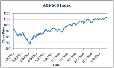
The second task is to estimate the parameters of the market-information process in Equation 11. The variable captures the potential impact of changing market conditions or private information about the security. can be described by the returns of a main index, e.g., the S&P 500 Index13, which behaves accordingly to market conditions.

We rescale the returns by subtracting out the mean and dividing by standard deviation. This yields to a zero-mean, unit standard-deviation process:

(29)

Once is an AR(1) process and assuming ,14 we can rewrite the standardized log returns as

(30)

The maximum likelihood estimator of the AR(1) coefficient, , is

(31)

13_{The S&P 500 Index measures changes in stock market conditions based on the average performance of} 500 widely held common stocks.

(42)

29 The constants, and , are the number of observations that are included in calculating the numerator and denominator.

is a measure of serial correlation – or autocorrelation – the correlation of a variable with itself over successive time intervals. If serial correlation exists implies that the correlation between and is not zero. Serial correlation determines how well the past price of a security predicts the future price.

Given , the maximum-likelihood estimator for the standard deviation of is (32)

The parameters and fully characterize the AR(1) process that describes the market-information.

5.5.3 Price-impact Equation

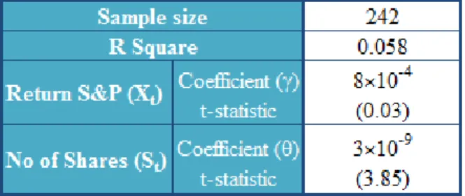
Our final assignment is to estimate the parameters  and  of the price-impact equation, rewriting Equation 8 (and using Equation 10) we obtain:

(33)

This expression shows that the percentage price impact is a linear function of the volume we intend to trade in the security, and the market information. As before, we form the no impact price, , as the average of the bid and ask (see Equation 28) and then construct the dependent variable,

(34) for each trade.

(43)

30

5.5.4 Risk Aversion Parameter

The risk aversion parameter (λ) indicates the weight placed on the price volatility component (which the portfolio is exposed during liquidation) compared to cost.

The risk aversion parameter can be either positive or negative.

If lambda is greater than zero, it would be chosen by a risk-averse trader who wishes to sell quickly to reduce exposure to volatility risk, despite the trading costs incurred in doing so.

When lambda is equal to zero, we‟ll call this the naive strategy, since it represents the optimal strategy corresponding to simply minimizing expected transaction costs without regard to variance (like the Bertsimas and Lo approach). Almgren and Chriss demonstrate that in a certain sense, this is never an optimal strategy, because one can obtain substantial reductions in variance for a relatively small increase in transaction costs.

When lambda is negative it would be chosen only by a trader who likes risk. He postpones selling, thus incurring lower expected trading costs but higher variance during the extended period that he holds the security.